Coordinated Weighted Sampling:
Estimation of Multiple-Assignment Aggregates

Abstract

Many data sources are naturally modeled by multiple weight assignments over a set of keys: snapshots of an evolving database at multiple points in time, measurements collected over multiple time periods, requests for resources served at multiple locations, and records with multiple numeric attributes. Over such vector-weighted data we are interested in aggregates with respect to one set of weights, such as weighted sums, and aggregates over multiple sets of weights such as the $L_{1}$ difference.

Sample-based summarization is highly effective for data sets that are too large to be stored or manipulated. The summary facilitates approximate processing of queries that may be specified after the summary was generated. Current designs, however, are geared for data sets where a single scalar weight is associated with each key.

We develop a sampling framework based on coordinated weighted samples that is suited for multiple weight assignments and obtain estimators that are orders of magnitude tighter than previously possible. We demonstrate the power of our methods through an extensive empirical evaluation on diverse data sets ranging from IP network to stock quotes data.

1 Introduction

Many business-critical applications today are based on extensive use of computing and communication network resources. These systems are instrumented to collect a wide range of different types of data. Examples include performance or environmental measurements, traffic traces, routing updates, or SNMP traps in an IP network, and transaction logs, system resource (CPU, memory) usage statistics, service level end-end performance statistics in an end- service infrastructure. Retrieval of useful information from this vast amount of data is critical to a wide range of compelling applications including network and service management, troubleshooting and root cause analysis, capacity provisioning, security, and sales and marketing.

Many of these data sources produce data sets consisting of numeric vectors (weight vectors) associated with a set of identifiers (keys) or equivalently as a set of weight assignments over keys. Aggregates over the data are specified using this abstraction.

We distinguish between data sources with co-located or dispersed weights. A data source has dispersed weights if entries of the weight vector of each key occur in different times or locations: (i) Snapshots of a database that is modified over time (each snapshot is a weight assignment, where the weight of a key is the value of a numeric attribute in a record with this key.) (ii) measurements of a set of parameters (keys) in different time periods (weight assignments). (iii) number of requests for different objects (keys) processed at multiple servers (weight assignments). A data source has co-located weights when a complete weight vector is “attached” to each key: (i) Records with multiple numeric attributes such as IP flow records generated by a statistics module at an IP router, where the attributes are the number of bytes, number of packets, and unit. (ii) Document-term datasets, where keys are documents and weight attributes are terms or features (The weight value of a term in a document can be the respective number of occurrences). (iii) Market-basket datasets, where keys are baskets and weight attributes are goods (The weight value of a good in a basket can be its multiplicity). (iv) Multiple numeric functions over one (or more) numeric measurement of a parameter. For example, for measurement $x$ we might be interested in both first and second moments, in which case we can use the weight assignments $x$ and $x^{2}$.

A very useful common type of query involves properties of a sub-population of the monitored data that are additive over keys. These aggregates can be broadly categorized as : (a) Single-assignment aggregates, defined with respect to a single attribute, such as the weighted sum or selectivity of a subpopulation of the keys. An example over IP flow records is the total bytes of all IP traffic with a certain destination Autonomous System [25, 1, 39, 16, 17]. (b) Multiple-assignment aggregates include similarity or divergence metrics such as the $L_{1}$ difference between two weight assignments or maximum/minimum weight over a subset of assignments [38, 22, 9, 21]. Figure 2 (A) shows an example of three weight assignments over a set of keys and key-wise values for multiple-assignment aggregates including the minimum or maximum value of a key over subset of assignments and the $L_{1}$ distance. The aggregate value over selected keys is the sum of key-wise values.

Multiple-assignment aggregates are used for clustering, change detection, and mining emerging patterns. Similarity over corpus of documents, according to a selected subset of features, can be used to detect near-duplicates and reduce redundancy [41, 10, 52, 20, 37, 42]. A retail merchant may want to cluster locations according to sales data for a certain type of merchandise. In IP networks, these aggregates are used for monitoring, security, and planning [28, 22, 23, 40]: An increase in the amount of distinct flows on a certain port might indicate a worm activity, increase in traffic to a certain set of destinations might indicate a flash crowd or a DDoS attack, and an increased number of flows from a certain source may indicate scanner activity. A network security application might track the increase in traffic to a customer site that originates from a certain suspicious network or geographic area.

Exact computation of such aggregates can be prohibitively resource-intensive: Data sets are often too large to be either stored for long time periods or to be collated across many locations. Computing multiple-assignment aggregates may require gleaning information across data sets from different times and locations. We therefore aim at concise summaries of the data sets, that can be computed in a scalable way and facilitate approximate query processing.

Sample-based summaries [36, 56, 7, 6, 11, 31, 32, 3, 24, 33, 17, 26, 14, 18] are more flexible than other formats: they naturally facilitate subpopulation queries by focusing on sampled keys that are members of the subpopulation and are suitable when the exact query of interest is not known beforehand or when there are multiple attributes of interest. When keys are weighted, weighted sampling, where heavier keys are more likely to be sampled, is essential for performance. Existing methods, however, are designed for one set of weights and are either not applicable or perform poorly on multiple-assignment aggregates.

Contributions

We develop sample-based summarization framework for vector-weighted data that supports efficient approximate aggregations. The challenges differ between the dispersed and co-located models due to the particular constraints imposed on scalable summarization.

Dispersed weights model: Any scalable algorithm must decouple the processing of different assignments – collating dispersed-weights data to obtain explicit key/vector-weight representation is too expensive. Hence, processing of one assignment can not depend on other assignments.

We propose summaries based on coordinated weighted samples. The summary contains a “classic” weighted sample taken with respect to each assignment. Coordination loosely means that a key that is sampled under one assignment is more likely to be sampled under other assignments. We can tailor the sampling to be Poisson, $k$-mins, or bottom-$k$ (order) sampling. In all three cases, sampling is efficient on data streams, distributed data, and metric data [11, 15, 27, 16] and there are unbiased subpopulation weight estimators that have variance that decreases linearly or faster with the sample size [11, 26, 54, 17]. Bottom-$k$ samples [47, 51, 48, 11, 17, 45, 26], with the advantage of a fixed sample size, emerge as a better choice. Our design has the following important properties:

$\bullet$

Scalability: The processing of each assignment is a simple adaptation of single-assignment weighted sampling algorithm. Coordination is achieved by using the same hash function across assignments.

$\bullet$

Weighted sample for each assignment: Our design is especially appealing for applications where sample-based summaries are already used, such as periodic (hourly) summaries of IP flow records. The use of our framework versus independent sampling in different periods facilitates support for queries on the relation of the data across time periods.

$\bullet$

Tight estimators: We provide a principled “template” derivation of estimators, tailor it to obtain tight unbiased estimators for the min, max, and range ($L_{1}$), and bound the variance.

Colocated weights model: For colocated data, the full weight vector of each key is readily available to the summarization algorithm and can be easily incorporated in the summary. We discuss the shortcomings of applying previous methods to summarize this data. One approach is to sample records according to one particular weight assignment. Such a sample can be used to estimate aggregates that involve other assignments, but estimates may have large variance and be biased. Another approach is to concurrently compute multiple weighted samples, one for each assignment. In this case, single-assignment aggregates can be computed over the respective sample but no unbiased estimators for multiple-assignment aggregates were known. Moreover, such a summary is wasteful in terms of storage as different assignments are often correlated (such as number of bytes and number of IP packets of an IP flow).

We consider summaries where the set of included keys embeds a weighted sample with respect to each assignment. The set of embedded samples can be independent or coordinated. Such a summary can be computed in a scalable way by a stream algorithm or distributively.

$\bullet$

We derive estimators, which we refer to as inclusive estimators, that utilize all keys included in the summary. An inclusive estimator of a single-assignment aggregate applied to a summary that embeds a certain weighted sample from that assignment is at least as tight, and typically significantly tighter, than an estimator directly applied to the embedded sample. Moreover, inclusive estimators are applicable to multiple-assignment aggregates, such as the $\min$, $\max$, and $L_{1}$.

$\bullet$

We show that when the embedded samples are coordinated, the number of distinct keys in the summary (in the union of the embedded samples) is minimized.

Empirical evaluation. We performed a comprehensive empirical evaluation using IP packet traces, movies’ ratings data set (The Netflix Challenge [44]), and stock quotes data set. These data sets and queries also demonstrate potential applications. For dispersed data we achieve orders of magnitude reduction in variance over previously-known estimators and estimators applied to independent weighted samples. The variance of these estimators is comparable to the variance of a weighted sum estimator of a single weight assignment.

For co-located data, we demonstrate that the size of our combined sample is significantly smaller than the sum of the sizes of independent samples one for each weight assignment. We also demonstrate that even for single assignment aggregates, our estimators which use the combined sample are much tighter than the estimators that use only a sample for the particular assignment.

Organization. The remainder of the paper is arranged as follows. Section  2 reviews related work, Section 3 presents key background concepts and Section 4 presents our sampling approach. Sections 5-7 present our estimators: Section 5 presents a template estimator which we apply to colocated summaries in Section 6 and to dispersed summaries in Section 7. Section 8 provides bounds on the variance. This is an extended version of [19].

2 Related work

Sample coordination. Sample coordination was used in survey sampling for almost four decades. Negative coordination in repeated surveys was used to decrease the likelihood that the same subject is surveyed (and burdened) multiple times. Positive coordination was used to make samples as similar as possible when parameters change in order to reduce overhead. Coordination is obtained using the PRN (Permanent Random Numbers) method for Poisson samples [5] and order (bottom-$k$) samples [50, 46, 48]. PRN resembles our “shared-seed” coordination method. The challenges of massive data sets, however, are different from those of survey sampling and in particular, we are not aware of previously existing unbiased estimators for multiple-assignment aggregates over coordinated weighted samples.

Coordination (of Poisson, $k$-mins, and bottom-$k$ samples) was (re-)introduced in computer science as a method to support aggregations that involve multiple sets [7, 6, 11, 31, 32, 3, 17, 33, 18] and as a form of locality sensitive hashing [9]. Coordination addressed the issue that independent samples of different sets over the same universe provide weak estimators for multiple-set aggregates such as intersection size or similarity. Intuitively, two large but almost identical sets are likely to have disjoint independent samples – the sampling does not retain any information on the relations between the sets.

This previous work, however, considered restricted weight models: uniform, where all weights are $0/1$, and global weights, where a key has the same weight value across all assignments where its weight is strictly positive (but the weight can vary between keys). Allowing the same key to assume different positive weights in different assignments is clearly essential for our applications.

While these methods can be applied with general weights, by ignoring weight values and performing coordinated uniform sampling, resulting estimators are weak. Intuiti vely, uniform sampling performs poorly on weighted data because it is likely to leave out keys with dominant weights. Weighted sampling, where keys with larger weights are more likely to be represented in the sample, is essential for boundable variance of weighted aggregates.

The structure of coordinated samples for general weights turns out to be more involved than with global weights, where essentially the samples of different assignments (sets) are derived from a single “global” (random) ranking of keys. The derivation of unbiased estimators was also more challenging: global weights allow us to make simple inferences on inclusion of keys in a set when the key is not represented in the sample. These inferences facilitate the derivation of estimators but do not hold under general weights.

Unaggregated data. Sample-based sketches [30, 13, 12] and sketches that are not samples were also proposed for unaggregated data streams (the scalar weight of each key appears in multiple data points) [2]. This is a more general model with weaker estimators than “aggregated” keys. We leave for future work summarization of unaggregated data set with vector-weights.

VarOpt is a weighted sampling design [8, 14] that realizes all the advantages of other schemes but it is not clear if it can be applied with coordinated samples (even with global weights).

Sketches that are not samples. Sketches that are not sample based [41, 10, 52, 20, 37, 42, 21, 29] are effective point solutions for particular metrics such as max-dominance [21] or $L_{1}$ [29] difference. Their disadvantage is less flexibility in terms of supported aggregates and in particular, no support for aggregates over selected subpopulations of keys: we can estimate the overall $L_{1}$ difference between two time periods but we can not estimate the difference restricted to a subpopulation such as flows to particular destination or certain application. There is also no mechanism to obtain “representatives” keys[53]. Lastly, even a practical implementation of [21, 29] involves constructions of stable distributions or range summable random variables (whereas for our sample-based summaries all is needed is “random-looking” hash functions).

Bloom filters [4, 28] also support estimation of similarity metrics but summary size is not tunable and grows linearly with the number of keys.

3 Preliminaries

weighted set $(I,w)$ with keys $I=\{i_{1},\ldots,i_{6}\}$ and a rank assignment r

key $i$:	$i_{1}$	$i_{2}$	$i_{3}$	$i_{4}$	$i_{5}$	$i_{6}$
weight $w(i)$	$20$	$10$	$12$	$20$	$10$	$10$
$u(i)\in U[0,1]$	$0.22$	$0.75$	$0.07$	$0.92$	$0.55$	$0.37$
$r(i)=u(i)/w(i)$	$0.011$	$0.075$	$0.0583$	$0.046$	$0.055$	$0.037$

Poisson samples with expected size $k=1,2,3$ and AW-summaries:
$p(i)=\min\{1,w(i)\tau\}$, $k=\sum_{i}p(i)$, $a(i)=w(i)/p(i)$

$k$	sample	$\tau$	$i:$	$i_{1}$	$i_{2}$	$i_{3}$	$i_{4}$	$i_{5}$	$i_{6}$
$1$	$i_{1}$	$\frac{1}{82}$	$p(i)$:	$0.24$	$0.12$	$0.15$	$0.24$	$0.12$	$0.12$
			$a(i)$:	$82$	$0$	$0$	$0$	$0$	$0$
$2$	$i_{1}$	$\frac{2}{82}$	$p(i)$:	$0.49$	$0.24$	$0.29$	$0.49$	$0.24$	$0.24$
			$a(i)$:	$41$	$0$	$0$	$0$	$0$	$0$
$3$	$i_{1}$	$\frac{3}{82}$	$p(i)$:	$0.73$	$0.37$	$0.44$	$0.73$	$0.37$	$0.37$
			$a(i)$:	$27.40$	$0$	$0$	$0$	$0$	$0$

Bottom-$k$ samples of size $k=1,2,3$ and AW-summaries:
$p(i)=\min\{1,w(i)r_{k+1}\}$, $a(i)=w(i)/p(i)$

$k$	sample	$r_{k+1}$	$i:$	$i_{1}$	$i_{2}$	$i_{3}$	$i_{4}$	$i_{5}$	$i_{6}$
$1$	$i_{1}$	$0.037$	$p(i)$:	$0.74$
			$a(i)$:	$27.02$	$0$	$0$	$0$	$0$	$0$
$2$	$i_{1},i_{6}$	$0.046$	$p(i)$:	$0.92$					$0.46$
			$a(i)$:	$21.74$	$0$	$0$	$0$	$0$	$21.74$
$3$	$i_{1},i_{6},i_{4}$	$0.055$	$p(i)$:	$1$			$1$		$0.55$
			$a(i)$:	$20.00$	$0$	$0$	$20.00$	$0$	$18.18$

Figure 1: Example of a weighted set, a random rank assignment with ipps ranks, Poisson and bottom-$k$ samples, and respective AW-summaries.

A weighted set $(I,w)$ consists of a set of keys $I$ and a function $w$ assigning a scalar weight value $w(i)\geq 0$ to each key $i\in I$. We review components of sample-based summarizations of a weighted set: sample distributions, respective sketches, that in our context are samples with some auxiliary information, and estimators for weight queries in the form of adjusted weights associated with sampled keys.

Sample distributions are defined through random rank assignments [11, 48, 16, 26, 17, 18] that map each key $i$ to a rank value $r(i)$. The rank assignment is defined with respect to a family of probability density functions ${\bf f}_{w}$ ($w\geq 0$), where each $r(i)$ is drawn independently according to ${\bf f}_{w(i)}$. We say that ${\bf f}_{w}$ ($w\geq 0$) are monotone if for all $w_{1}\geq w_{2}$, for all $x$, ${\bf F}_{w_{1}}(x)\geq{\bf F}_{w_{2}}(x)$ (where $\bf{F}_{w}$ are the respective cumulative distributions). For a set $J$ and a rank assignment $r$ we denote by $r_{i}(J)$ the $i$th smallest rank of a key in $J$, we also abbreviate and write $r(J)=r_{1}(J)$.

$\bullet$

A Poisson-$\tau$ sample of $J$ is defined with respect to a rank assignment $r$. The sample is the set of keys with $r(i)<\tau$. The sample has expected size $k=\sum_{i}{\bf F}_{w(i)}(\tau)$. Keys have independent inclusion probabilities. The sketch includes the pairs $(r(i),w(i))$ and may include key identifiers with attribute values.

$\bullet$

A bottom-$k$ (order-$k$) sample of $J$ contains the $k$ keys $i_{1},\ldots,i_{k}$ of smallest ranks in $J$. The sketch $s_{k}(J,r)$ consists of the $k$ pairs $(r(i_{j}),w(i_{j}))$, $j=1,\ldots,k$, and $r_{k+1}(J)$. (If $|J|\leq k$ we store only $|J|$ pairs.), and may include the key identifiers $i_{j}$ and additional attributes.

$\bullet$

A $k$-mins sample of $J\subset I$ is produced from $k$ independent rank assignments, $r^{(1)},\ldots,r^{(k)}$. The sample is the set of (at most $k$) keys) with minimum rank values $r^{(1)}(J)$, $r^{(2)}(J)$, $\ldots$, $r^{(k)}(J)$. The sketch includes the minimum rank values and, depending on the application, may include corresponding key identifiers and attribute values.

When weights of keys are uniform, a $k$-mins sample is the result of $k$ uniform draws with replacement, bottom-$k$ samples are $k$ uniform draws without replacements, and Poisson-$\tau$ samples are independent Bernoulli trials. The particular family ${\bf f}_{w}$ matters when weights are not uniform. Two families with special properties are:

$\bullet$

exp ranks: ${\bf f}_{w}(x)=we^{-wx}$ (${\bf F}_{w}(x)=1-e^{-wx}$) are exponentially-distributed with parameter $w$ (denoted by $\mbox{\sc exp}[w]$). Equivalently, if $u\in U[0,1]$ then $-\ln(u)/w$ is an exponential random variable with parameter $w$. $\mbox{\sc exp}[w]$ ranks have the property that the minimum rank $r(J)$ has distribution $\mbox{\sc exp}[w(J)]$, where $w(J)=\sum_{i\in J}w(i)$. (The minimum of independent exponentially distributed random variables is exponentially distributed with parameter equal to the sum of the parameters of these distributions). This property is useful for designing estimators and efficiently computing sketches [11, 15, 27, 16, 17]. The $k$-mins sample [11] of a set is a sample drawn with replacement in $k$ draws where a key is selected with probability equal to the ratio of its weight and the total weight. A bottom-$k$ sample is the result of $k$ such draws performed without replacement, where keys are selected according to the ratio of their weight and the weight of remaining keys [47, 34, 48].

$\bullet$

ipps ranks: ${\bf f}_{w}$ is the uniform distribution $U[0,1/w]$ (${\bf F}_{w}(x)=\min\{1,wx\}$). This is the equivalent to choosing rank value $u/w$, where $u\in U[0,1]$. The Poisson-$\tau$ sample is an ipps sample [34] (Inclusion Probability Proportional to Size). The bottom-$k$ sample is a priority sample [45, 26] (pri).

Figure 1 shows an example of a weighted set with 6 keys and a respective rank assignment with ipps ranks. The figure shows the corresponding Poisson samples of expected size $k=1,2,3$. The value $\tau$ is calculated according to the desired expected sample size. The sample includes all keys with rank value that is below $\tau$. This particular rank assignment yielded a Poisson sample of size $1$ when the expected size was $1,2,3$. The figure also shows bottom-$k$ samples of sizes $k=1,2,3$, containing the $k$ keys with smallest rank values.

Adjusted weights. A technique to obtain estimators for the weights of keys is by assigning an adjusted weight $a(i)\geq 0$ to each key $i$ in the sample (adjusted weight $a(i)=0$ is implicitly assigned to keys not in the sample). The adjusted weights are assigned such that ${\textsf{E}}[a(i)]=w(i)$, where the expectation is over the randomized algorithm choosing the sample. We refer to the (random variable) that combines a weighted sample of $(I,w)$ together with adjusted weights as an adjusted-weights summary (AW-summary) of $(I,w)$. An AW-summary allows us to obtain an unbiased estimate on the weight of any subpopulation $J\subset I$. The estimate $\sum_{j\in J}a(j)=\sum_{j\in J|a(j)>0}a(j)$ is easily computed from the summary provided that we have sufficient auxiliary information to tell for each key in the summary whether it belongs to $J$ or not. Figure 1 shows example AW-summaries for the Poisson and bottom-$k$ samples. The set $J=\{i_{2},i_{4},i_{6}\}$ with weight $w(J)=w(i_{2})+w(i_{4})+w(i_{6})=10+20+10=40$ has estimate of $0$ using the three Poisson AW-summaries and estimates $0,21.74,38.18$ respectively by the three bottom-$k$ AW-summaries. Moreover, for any secondary numeric function $h()$ over keys’ attributes such that $h(i)>0\implies w(i)>0$ and any subpopulation $J$, $\sum_{j\in J|a(j)>0}a(j)h(j)/w(j)$ is an unbiased estimate of $\sum_{j\in J}h(j)$.

Horvitz-Thompson (HT). Let $\Omega$ be the distribution over samples such that if $w(i)>0$ then $p^{(\Omega)}(i)=\Pr\{i\in s|s\in\Omega\}$ is positive. If we know $p^{(\Omega)}(i)$ for every $i\in s$, we can assign to $i\in s$ the adjusted weight $a(i)=\frac{w(i)}{p^{(\Omega)}(i)}\ .$ Since $a(i)$ is $0$ when $i\not\in s$, ${\textsf{E}}[a(i)]=w(i)$ ($a(i)$ is an unbiased estimator of $w(i)$). These adjusted weights are called the Horvitz-Thompson (HT) estimator [35]. For a particular $\Omega$, the HT adjusted weights minimize $\mbox{\sc var}[a(i)]$ for all $i\in I$. The HT adjusted weights for Poisson $\tau$-sampling are $a(i)=w(i)/{\bf F}_{w(i)}(\tau)$. Figure 1 shows the inclusion probability ${\bf F}_{w(i)}(\tau)$ and a corresponding AW-summary for the Poisson samples. Poisson sampling with ipps ranks and HT adjusted weights are known to minimize the sum $\sum_{i\in I}\mbox{\sc var}(a(i))$ of per-key variances over all AW-summaries with the same expected size.

HT on a partitioned sample space (HTp) [17]. This is a method to derive adjusted weights when we cannot determine $\Pr\{i\in s|s\in\Omega\}$ from the information contained in the sketch $s$ alone.

For each key $i$ we consider a partition of $\Omega$ into equivalence classes. For a sketch $s$, let $P^{i}(s)\subset\Omega$ be the equivalence class of $s$. This partition must satisfy the following requirement: Given $s$ such that $i\in s$, we can compute the conditional probability $p^{i}(s)=\Pr\{i\in s^{\prime}\mid s^{\prime}\in P^{i}(s)\}$ from the information included in $s$.

We can therefore compute for all $i\in s$ the assignment $a(i)=w(i)/p^{i}(s)$ (implicitly, $a(i)=0$ for $i\not\in s$.) It is easy to see that within each equivalence class, ${\textsf{E}}[a(i)]=w(i)$. Therefore, also over $\Omega$ we have ${\textsf{E}}[a(i)]=w(i)$.

Rank Conditioning (RC) [[17]]. When $s$ is a bottom-$k$ sketch of $(I,w)$, then $\Pr\{i\in s|s\in\Omega\}$ generally depends on all the weights $w(i)$ for $i\in I$ and therefore cannot be determined from $s$. Therefore, we can not directly apply the HT estimator. RC is an HTp method designed for bottom-$k$ sketches. For each $i$ and possible rank value $\tau$ we have an equivalence class $P^{i}_{\tau}$ containing all sketches in which the $k$th smallest rank value assigned to a key other than $i$ is $\tau$. Note that if $i\in s$ then $\tau$ is the $(k+1)$st smallest rank which is included in the sketch. The inclusion probability of $i$ in a sketch in $P^{i}_{\tau}$ is $p^{i}_{\tau}={\bf F}_{w(i)}(\tau)$ and it can be computed from the sample.

Applying RC, consider $s$ containing keys $i_{1},\ldots,i_{k}$ and the $(k+1)$st smallest rank value $r_{k+1}$. Then for key $i_{j}$, we have $s\in P^{i_{j}}_{r_{k+1}}$ and $a(i_{j})=\frac{w(i_{j})}{\mbox{\bf F}_{w(i_{j})}(r_{k+1})}$. The RC estimator for bottom-$k$ samples with ipps ranks [26] has a sum of per-key variances that is at most that of an HT estimator applied to a Poisson sample with ipps ranks and expected size $k+1$ [54].

This RC method was extended in [18] to obtain estimators over coordinated bottom-$k$ sketches with global weights [18]. The RC method facilitated the derivation and analysis of unbiased estimators over bottom-$k$ samples – it provided a way to “get around” the dependence between inclusions of different keys, typically, without sacrificing accuracy with respect to estimators over Poisson samples.

Figure 1 shows the $(k+1)$st smallest rank value, the conditional inclusion probability ${\bf F}_{w(i)}(r_{k+1})$ and the corresponding AW-summary for each bottom-$k$ sample in the example.

We subsequently use the notation $\Omega(i,r^{-i})$ for the probability subspace of rank assignments that contains all rank assignments $r^{\prime}$ that agree on $r$ for all keys in $I\setminus\{i\}$.

Sum of per-key variances Different AW-summaries are compared based on their estimation quality. Variance is the standard metric for the quality of an estimator for a single quantity. For a subpopulation $J$ and AW-summaries $a()$, the variance is $\mbox{\sc var}[a(J)]={\textsf{E}}[a(J)]^{2}-w(J)^{2}$. Since our application is for subpopulations that may not be specified a priori, the notion of a good metric is more subtle. Clearly there is no single AW-summary that dominates all others of the same size (minimizes the variance) for all subpopulations $J$.

The metric we use in our performance evaluation is the sum of per-key variances ${\Sigma}V[a]\equiv\sum_{i\in I}\mbox{\sc var}[a(i)]$ [26, 17]. For AW-summaries with zero covariances (for any two keys $i,j$, $\mbox{\sc cov}[a(i),a(j)]={\textsf{E}}[a(i)a(j)]-w(i)w(j)=0$), ${\Sigma}V[a]$ also measures average variance over subpopulations of any given weight or size [55]. RC adjusted weights on single-assignment [17] and their extension to coordinated sketches with global weights [18] have zero covariances. HT adjusted weights for Poisson sketches have zero covariances (this is immediate from independence). When covariances are zero, the variance of $a(J)$ for a particular subpopulation $J$ is equal to $\sum_{i,j\in J}\mbox{\sc cov}[a(i),a(j)]=\sum_{i\in J}\mbox{\sc var}[a(i)]$.

Estimators for Poisson, $k$-mins, and bottom-$k$ sketches with exp or ipps ranks have ${\Sigma}V[a]\leq\frac{w(I)^{2}}{k-2}$ (where $k$ is the (expected) sample size) [11, 16, 26, 54]. For a subpopulation $J$ with expected $k^{\prime}$ samples in the sketch, the variance on estimating $w(J)$ is bounded by $w(J)^{2}/(k^{\prime}-2)$. For bottom-$k$ and Poisson sketches, the variance is smaller when the weight distribution is more skewed  [16, 26].

4 Model and summary formats

We model the data using a set of keys $I$ and a set ${\cal W}$ of weight assignments over $I$. For each $b\in{\cal W}$, $w^{(b)}:I\rightarrow{\cal{R}}_{\geq 0}$ maps keys to nonnegative reals. Figure 2 shows a data set with $I=\{i_{1},\ldots,i_{6}\}$ and ${\cal W}=\{1,2,3\}$. For $i\in I$ and ${\cal R}\subset{\cal W}$, we use the notation $w^{({\cal R})}(i)$ for the weight vector with entries $w^{(b)}(i)$ ordered by $b\in{\cal R}$.

keys: $I=\{i_{1},\ldots,i_{6}\}$

weight assignments: $w^{(1)},w^{(2)},w^{(3)}$

assignment/key	$i_{1}$	$i_{2}$	$i_{3}$	$i_{4}$	$i_{5}$	$i_{6}$
$w^{(1)}$	15	0	10	5	10	10
$w^{(2)}$	20	10	12	20	0	10
$w^{(3)}$	10	15	15	0	15	10
Example functions $f(i_{j})$
$w^{(\max\{1,2\})}$	20	10	12	20	10	10
$w^{(\max\{1,2,3\})}$	20	15	15	20	15	10
$w^{(\min\{1,2\})}$	15	0	10	0	0	10
$w^{(\min\{1,2,3\})}$	10	0	10	0	0	10
$w^{(L_{1}\{1,2\})}$	5	10	2	15	10	0
$w^{(L_{1}\{2,3\})}$	10	5	3	20	15	0

(A)

Consistent shared-seed ipps ranks:
key: $i_{1}$ $i_{2}$ $i_{3}$ $i_{4}$ $i_{5}$ $i_{6}$ $u$ $0.22$ $0.75$ $0.07$ $0.92$ $0.55$ $0.37$ $r^{(1)}$ $0.0147$ $+\infty$ $0.007$ $0.184$ $0.055$ $0.037$ $r^{(2)}$ $0.011$ $0.075$ $0.0583$ $0.046$ $+\infty$ $0.037$ $r^{(3)}$ $0.022$ $0.05$ $0.0047$ $+\infty$ $0.0367$ $0.037$

Independent ipps ranks:
key: $i_{1}$ $i_{2}$ $i_{3}$ $i_{4}$ $i_{5}$ $i_{6}$ $u^{(1)}$ $0.22$ $0.75$ $0.07$ $0.92$ $0.55$ $0.37$ $r^{(1)}$ $0.0147$ $+\infty$ $0.007$ $0.184$ $0.055$ $0.037$ $u^{(2)}$ $0.47$ $0.58$ $0.71$ $0.84$ $0.25$ $0.32$ $r^{(2)}$ $0.0235$ $0.058$ $0.0592$ $0.042$ $+\infty$ $0.032$ $u^{(3)}$ $0.63$ $0.92$ $0.08$ $0.59$ $0.32$ $0.80$ $r^{(3)}$ $0.063$ $0.0613$ $0.0053$ $+\infty$ $0.0213$ $0.08$

(B)

bottom-$3$ samples:

$w^{(1)}$	$i_{3}$, $i_{1}$, $i_{6}$
$w^{(2)}$	$i_{1}$, $i_{6}$, $i_{4}$
$w^{(3)}$	$i_{3}$, $i_{1}$, $i_{5}$

bottom-$3$ samples:

$w^{(1)}$	$i_{3}$, $i_{1}$, $i_{6}$
$w^{(2)}$	$i_{1}$, $i_{6}$, $i_{4}$
$w^{(3)}$	$i_{3}$, $i_{5}$, $i_{2}$

Figure 2: (A): Example data set with keys $I=\{i_{1},\ldots,i_{6}\}$ and weight assignments $w^{(1)},w^{(2)},w^{(3)}$ and per-key values for example aggregates. (B): random rank assignments and corresponding bottom-$3$ samples.

We are interested in aggregates of the form $\sum_{i|d(i)=1}f(i)$ where $d$ is a selection predicate and $f$ is a numeric function, both defined over the set of keys $I$. $f(i)$ and $d(i)$ may depend on the attribute values associated with key $i$ and on the weight vector $w^{({\cal W})}(i)$.

We say that the function $f$/predicate $d$ is single-assignment if it depends on $w^{(b)}(i)$ for a single $b\in{\cal W}$. Otherwise we say that it is multiple-assignment. The relevant assignments of $f$ and $d$ are those necessary for determining all keys $i$ such that $d(i)=1$ and evaluating $f(i)$ for these keys.

The maximum and minimum with respect to a set of assignments ${\cal R}\subset{\cal W}$, are defined by $f(i)$ as follows:

$$w^{(\max{\cal R})}(i)\equiv\max_{b\in{\cal R}}w^{(b)}(i)\;\;\;\;w^{(\min{\cal R})}(i)\equiv\min_{b\in{\cal R}}w^{(b)}(i)\ .$$ (1)

The relevant assignments for $f$ in this case are ${\cal R}$. Sums over these $f$’s are also known as the max-dominance and min-dominance norms [21, 22] of the selected subset. The maximum reduces to the size of set union and the minimum to the size of set intersection for the special case of global weights.

The ratio ${\sum_{i\in J}w^{(\min{\cal R})}(i)}/{\sum_{i\in J}w^{(\max{\cal R})}(i)}$ when $|{\cal R}|=2$ is the weighted Jaccard similarity of the assignments ${\cal R}$ on $J$. The range ($L_{1}$ difference when $|{\cal R}|=2$) can be expressed as a sum aggregate by choosing $f(i)$ to be

$$w^{(L_{1}{\cal R})}(i)\equiv w^{(\max{\cal R})}(i)-w^{(\min{\cal R})}(i)\ .$$ (2)

For the example in Figure 2, the max dominance norm over even keys (specified by a predicate $d$ that is true for $i_{2},i_{4},i_{6}$) and assignments ${\cal R}=\{1,2,3\}$ is $w^{(\max\{1,2,3\})}(i_{2})+w^{(\max\{1,2,3\})}(i_{4})+w^{(\max\{1,2,3\})}(i_{6})=15+20+10=45$, the $L_{1}$ distance between assignments ${\cal R}=\{2,3\}$ over keys $i_{1},i_{2},i_{3}$ is $w^{(L_{1}\{2,3\})}(i_{1})+w^{(L_{1}\{2,3\})}(i_{2})+w^{(L_{1}\{2,3\})}(i_{3})=10+5+3=18$.

This classification of dispersed and colocated models differentiates the summary formats that can be computed in a scalable way: With colocated weights, each key is processed once, and samples for different assignments $b\in{\cal W}$ are generated together and can be coupled. Moreover, the (full) weight vector can be easily incorporated with each key included in the final summary. With dispersed weights, any scalable summarization algorithm must decouple the sampling for different $b\in{\cal W}$. The process and result for $b\in{\cal W}$ can only depend on the values $w^{(b)}(i)$ for $i\in I$. The final summary is generated from the results of these disjoint processes.

Random rank assignments for $(I,{\cal W})$. A random rank assignment for $(I,{\cal W})$ associates a rank value $r^{(b)}(i)$ for each $i\in I$ and $b\in{\cal W}$. If $w^{(b)}(i)=0$, $r^{(b)}(i)=+\infty$. The rank vector of $i\in I$, $r^{({\cal W})}(i)$, has entries $r^{(b)}(i)$ ordered by $b\in{\cal W}$. The distribution $\Omega$ is defined with respect to a monotone family of density functions $\bf{f}_{w}$ ($w\geq 0$) and has the following properties: (i) For all $b$ and $i$ such that $w^{(b)}(i)>0$, the distribution of $r^{(b)}(i)$ is $\bf{f}_{w^{(b)}(i)}$. (ii) The rank vectors $r^{({\cal W})}(i)$ for $i\in I$ are independent. (iii) For all $i\in I$, the distribution of the rank vector $r^{({\cal W})}(i)$ depends only on the weight vector $w^{({\cal W})}(i)$.

It follows from (i) and (ii) that for each $b\in{\cal W}$, $\{r^{(b)}(i)|i\in I\}$ is a random rank assignment for the weighted set $(I,w^{(b)})$ with respect to the family $\bf{f}_{w}$ ($w\geq 0$). The distribution $\Omega$ is specified by the mapping (iii) from weight vectors to distributions of rank vectors specifies $\Omega$.

Independent or consistent ranks. If for each key $i$, the entries $r^{(b)}(i)$ ($b\in{\cal W}$) of the rank vector of $i$ are independent we say that the rank assignment has independent ranks. In this case $\Omega$ is the product distribution of independent rank assignments $r^{(b)}$ for $(I,w^{(b)})$ ($b\in{\cal W}$).

A rank assignment has consistent ranks if for each key $i\in I$ and any two weight assignments $b_{1},b_{2}\in{\cal W}$,

$$w^{(b_{1})}(i)\geq w^{(b_{2})}(i)\Rightarrow r^{(b_{1})}(i)\leq r^{(b_{2})}(i)\ .$$

(in particular, if entries of the weight vector are equal then corresponding rank values are equal, that is, $w^{(b_{1})}(i)=w^{(b_{2})}(i)\Rightarrow r^{(b_{1})}(i)=r^{(b_{2})}(i)$.)

In the special case of global (or uniform) weights, consistency means that the entries of each rank vector are equal and distributed according to ${\bf f}_{w(i)}$ for all $b\in{\cal W}$ such that $w^{(b)}(i)>0$. Therefore, the distribution of the rank vectors is determined uniquely by the family ${\bf f}_{w}$ ($w>0$). This is not true for general weights. We explore the following two distributions of consistent ranks, specified by a mapping of weight vectors to probability distributions of rank vectors.

$\bullet$ Shared-seed: Independently, for each key $i\in I$:
$\bullet$ $u(i)\leftarrow U[0,1]$ (where $U[0,1]$ is the uniform distribution on $[0,1]$.)
$\bullet$ For $b\in{\cal W}$, $r^{(b)}(i)\leftarrow{\bf F}^{-1}_{w^{(b)}(i)}(u(i))$.

That is, for $i\in I$, $r^{(b)}(i)$ ($b\in{\cal W}$) are determined using the same “placement” ($u(i)$) in ${\bf F}_{w^{(b)}(i)}$.

Consistency of this construction is an immediate consequence of the monotonicity property of ${\bf f}_{w}$.

Shared-seed assignment for ipps ranks is $r^{(b)}(i)=u(i)/w^{(b)}(i)$ and for exp ranks, is $r^{(b)}(i)=-\ln(1-u(i))/w^{(b)}(i)$.

$\bullet$ Independent-differences is specific to exp ranks. Recall that $\mbox{\sc exp}[w]$ denotes the exponential distribution with parameter $w$. Independently, for each key $i$:
Let $w^{(b_{1})}(i)\leq\cdots\leq w^{(b_{h})}(i)$ be the entries of the weight vector of $i$.
$~{}\quad\bullet$ For $j\in 1\ldots h$, $d_{j}\leftarrow\mbox{\sc exp}[w^{(b_{j})}(i)-w^{(b_{j-1})}(i)]$, where $w^{(0)}(i)\equiv 0$ and $d_{j}$ are independent.
$~{}\quad\bullet$ For $j\in 1\ldots h$, $r^{(b_{j})}(i)\leftarrow\min_{a=1}^{j}d_{j}$.

For these ranks consistency is immediate from the construction. Since the distribution of the minimum of independent exponential random variables is exponential with parameter that is equal to the sum of the parameters, we have that for all $b\in{\cal W}$, $i\in I$, $r^{(b)}(i)$ is exponentially distributed with parameter $w^{(b)}(i)$.

Coordinated and independent sketches. Coordinated sketches are derived from assignments with consistent ranks and independent sketches from assignments with independent ranks. $k$-mins sketches: An ordered set of $k$ rank assignments for $(I,{\cal W})$ defines a set of $|{\cal W}|$ $k$-mins sketches, one for each assignment $b\in{\cal W}$. Bottom-$k$ and Poisson sketches: A single rank assignment $r$ on $(I,{\cal W})$ defines a bottom-$k$ sketch (and a Poisson $\tau^{(b)}$-sketch) for each $b\in{\cal W}$, (using the rank values $\{r^{(b)}(i)|i\in I\}$). Figure 2 shows examples of independent and shared-seed consistent rank assignments for the example data set and the corresponding bottom-$3$ samples.

Independent differences ranks allow for a generalization of the estimator for unweighted Jaccard similarity [6]:

Theorem 4.1.

$k$-mins sketches derived from rank assignments with independent-differences consistent ranks have the following property: For any $b_{1},b_{2}\in{\cal W}$, the probability that both assignments have the same minimum-rank key is equal to the weighted Jaccard similarity of the two weight assignments.

Proof.

Let ${\cal R}=\{b_{1},b_{2}\}$. Independent differences rank distribution is equivalent to drawing (independently) two exponentially distributed random variables for each key $i$, $r^{\prime}(i)$ and $r^{\prime\prime}(i)$ according to weights $w^{(\min{\cal R})}(i)$ and $w^{(L_{1}\ {\cal R})}(i)$. If $w^{(b_{h})}(i)=\min\{w^{(b_{1})}(i),w^{(b_{2})}(i)\}$ we set $r^{(b_{h})}(i)\leftarrow r^{\prime}(i)$ and otherwise $r^{(b_{h})}(i)\leftarrow\min\{r^{\prime}(i),r^{\prime\prime}(i)\}$. This follows from the property that the minimum of independent and exponentially distributed variables is exponentially distributed with parameter equal to the sum of the parameters.

To establish the lemma, we need to show that

$$\mbox{\sc pr}[\min_{i}r^{(b_{1})}(i)=\min_{i}r^{(b_{2})}(i)]=\mbox{\sc pr}[\min_{i}r^{\prime}(i)<\min_{i}r^{\prime\prime}(i)]\ .$$

We again use the property that the minimum of independent and exponentially distributed variables is exponentially distributed with the sum of the parameters. Hence, $\min_{i}r^{\prime}(i)$ and $\min_{i}r^{\prime\prime}(i)$ are independent and exponentially distributed with parameters $\sum_{i}w^{(\min{\cal R})}(i)$ and $\sum_{i}w^{(L_{1}\ {\cal R})}(i)$, respectively. Therefore,

$$\mbox{\sc pr}[\min_{i}r^{\prime}(i)<\min_{i}r^{\prime\prime}(i)]=\frac{\sum_{i}w^{(\min{\cal R})}(i)}{\sum_{i}w^{(\min{\cal R})}(i)+\sum_{i}w^{(L_{1}\ {\cal R})}(i)}=\frac{\sum_{i}w^{(\min{\cal R})}(i)}{\sum_{i}w^{(\max{\cal R})}(i)}\ .$$

The last equality is correct because for two independent exponentially distributed random variables with parameters $y_{1},y_{2}$, the probability that the $i$th is smaller is $y_{i}/(y_{1}+y_{2})$. ∎

It follows that the fraction of common keys in the two $k$-mins sketches is an unbiased estimator of the weighted Jaccard similarity of the two assignments.

For Poisson sketches, shared-seed consistent ranks maximize the sharing of keys between sketches. In fact, they are the only joint distribution over assignments that does so. We conjecture that this holds also for bottom-$k$ and $k$-mins sketches.

Theorem 4.2.

Consider all distributions of rank assignments on $(I,{\cal W})$ obtained using a family ${\bf F}_{w}$. Shared-seed consistent ranks (is the unique rank distribution that) minimize the expected number of distinct keys in the union of the sketches for $(I,w^{(b)})$, $b\in{\cal W}$.

Proof.

We first consider Poisson sketches. Consider Poisson-$\tau^{(b)}$ sketches ($b\in{\cal R}$). Since the inclusion of different keys are independent, it suffices to show the claim for a single key $i$. Let $p^{(b)}={\bf F}_{w^{(b)}(i)}(\tau^{(b)})$. With any distribution of rank assignments, the probability that $i$ is included in at least one sketch for $b\in{\cal R}$ is at least $\max_{b\in{\cal R}}p^{(b)}$. With shared-seed ranks, this probability equals $\max_{b\in{\cal R}}p^{(b)}$, and hence, it is minimized.

For bottom-$k$ sketches, there is no joint distribution with the property that the inclusion probability of a key in at least one sketch is equal to its maximum inclusion probability over sketches ($b\in{\cal R}$). What we can show is that shared-seed is optimal for a key $i$ when fixing the distribution of $r(I\setminus\{i\})$. The argument uses the independence of the rank vectors of different keys. Specifically, for each key $i$, the joint distribution of $\tau^{(b)}=r^{(b)}_{k}(I\setminus\{i\})$ ($b\in{\cal R}$) is independent of the joint distribution of $r^{(b)}(i)$ ($b\in{\cal R}$). Thus, conditioned on the outcome of $r^{(b)}_{k}(I\setminus\{i\})$ ($b\in{\cal R}$), the inclusion probability of $i$ in the sketch of $b$ is $p^{(b)}={\bf F}_{w^{(b)}(i)}(\tau^{(b)})$. We can now reuse the argument for Poisson sketches to show that with shared-seed ranks, $i$ is included in at least one sketch from ${\cal R}$ with probability exactly $\max_{b\in{\cal R}}p^{(b)}$. Hence, this choice is optimal under this conditioning.

∎

Sketches for the maximum weight. For ${\cal R}\subset{\cal W}$, let $r^{(\min{\cal R})}(i)=\min_{b\in{\cal R}}r^{(b)}(i)$. The following holds for all consistent rank assignments:

Lemma 4.1.

Let $r$ be a consistent rank assignment for $(I,{\cal W})$ with respect to ${\bf f}_{w}$ ($w>0$). Let ${\cal R}\subset{\cal W}$. Then $r^{(\min{\cal R})}(i)$ is a rank assignment for the weighted set $(I,w^{(\max{\cal R})})$ with respect to ${\bf f}_{w}$ ($w>0$).

Proof.

From the definition of consistency, $r^{(\min{\cal R})}(i)\equiv r^{(b)}(i)$ where $b=\arg\max_{b\in{\cal R}}w^{(b)}(i)$. Therefore, the distribution of $r^{(\min{\cal R})}(i)$ is ${\bf f}_{w^{(\max{\cal R})}(i)}$. It remains to show that $\{r^{(\min{\cal R})}(i)|i\in I\}$ are independent. This immediately follows from the definition of a rank assignment: if sets of random variables are independent (rank vectors of different keys), so are the respective maxima. ∎

A consequence of Lemma 4.1 is the following:

Lemma 4.2.

From coordinated Poisson $\tau^{(b)}$-/bottom-$k$-/$k$-mins sketches for ${\cal R}\subset{\cal W}$, we can obtain a Poisson $\min_{b\in{\cal R}}\tau^{(b)}$-/bottom-$k$-/$k$-mins sketch for $(I,w^{(\max{\cal R})})$.

Proof.

$k$-mins sketches: we take the coordinate-wise minima (and respective keys) of the $k$-mins sketch vectors of $(I,w^{(b)})$, $b\in{\cal R}$.

Given a rank assignment $r$ for $(I,{\cal W})$ then by Lemma 4.1 $r^{(\min{\cal R})}(i)$ is a rank assignment for $(I,w^{(\max{\cal R})})$. So by the definition of a $k$-mins sketch we should take the key achieving $\min_{i\in I}r^{(\min{\cal R})}(i)$ to the $k$-mins sketch of $(I,w^{(\max{\cal R})})$, and repeat this for $k$ different rank assignments.

Let $j_{b}$ be the key such that $r^{(b)}(j_{b})$ is minimum among all $r^{(b)}(i)$. The lemma follows since

$$\min_{b\in{\cal R}}r^{(b)}(j_{b})=\min_{b\in{\cal R}}\min_{i\in I}r^{(b)}(i)=\min_{i\in I}\min_{b\in{\cal R}}r^{(b)}(i)=\min_{i\in I}r^{(\min{\cal R})}(i)\ .$$

Poisson $\tau^{(b)}$-sketches: we include all keys with rank value at most $\min_{b\in{\cal R}}\tau^{(b)}$ in the union of the sketches.

Bottom-$k$ sketches: we take the $k$ distinct keys with smallest rank values in the union of the sketches. The proof is deferred and is a consequence of Lemma 7.2. ∎

This property of coordinated sketches generalizes the union-sketch property of coordinated sketches for global and uniform weights, which facilitates multiple-set aggregates [11, 7, 6, 17, 18].

Fixed number of distinct keys for colocated data. The number of distinct keys in a set of bottom-$k$ sketches of different assignments is between $k$ and $|{\cal W}|k$. It is closer to $k$ with coordination of sketches and similarity of assignments. Therefore, even though $k$, which is the size of each embedded sample, is fixed the total size varies. A natural goal under storage constraints is to fix the number of distinct keys in the combined sample.

For a rank assignment $r$, we choose $\ell$ ($\ell\geq k$) to be the largest such that there are at most $|{\cal W}|k$ distinct keys in the union of the bottom-$\ell$ samples taken with respect to $r^{(b)}$ ($b\in{\cal W}$). The total number of distinct keys is at least $|{\cal W}|(k-1)+1$. Such a sample can be computed by a simple adaptation of the stream sampling algorithm for the fixed-$k$ variant. For Poisson sketches, we can similarly fix the expected size of the combined samples, a stream algorithm can similarly select $\tau^{(b)}$ adaptively so that the expected size of each embedded sample is at least $\ell\geq k$ and the expected total size is in $[|{\cal W}|(k-1)+1,|{\cal W}|k]$.

In the sequel we develop estimators over bottom-$k$ sketches. The treatment of Poisson sketches is similar and simpler. Derivations extend easily to bottom-$k^{(b)}$ sketches (with different sizes for different assignments) and to colocated data sketches with fixed number of distinct keys. We shall denote by $S(r)$ the summary consisting of $|{\cal W}|$ bottom-$k$ sketches obtained using a rank assignment $r$.

Computing coordinated sketches. Coordinated bottom-$k$ sketches can be computed by a small modification of existing bottom-$k$ sampling algorithms. If weights are colocated the computation is simple (for both shared-seed and independent-differences), as each key is processed once. For dispersed weights and shared-seed, random hash functions must be used to ensure that the same seed $u(i)$ is used for the key $i$ in different assignments. We apply the common practice of assuming perfect randomness of the rank assignment in the analysis. This practice is justified by a general phenomenon [49, 43], that simple heuristic hash functions and pseudo-random number generators [3] perform in practice as predicted by this simplified analysis. This phenomenon is also supported by our evaluation.

Independent-differences are not suited for dispersed weights as they require range summable universal hash functions [29, 49].

5 Template Estimator

Consider $(I,{\cal W})$ a sample space of rank assignments $\Omega$, and a summary $S$.

We present an unbiased template estimator for sum aggregates $\sum_{i\in I|d(i)=1}f(i)$ (where $f$ is a numeric function $f$ $d$ is a predicate $d$). The template estimator is an adaptation of the HT estimator to our multiple-assignments setting.

The template estimator assigns adjusted $f$-weights $a^{(f)}(i)\geq 0$ to the keys (we have implicit zero adjusted weights $a^{(f)}(i)\equiv 0$ for $i\not\in S$). The estimate on $\sum_{i|d(i)=1}f(i)$ is the sum $\sum_{i\in S\mid d(i)=1}a^{(f)}(i)$ of the adjusted $f$-weights of keys in $S$ that satisfy the predicate $d$.

We subsequently apply this template to different summary types (colocated or dispersed weights), independent or coordinated distributions of rank assignments, and $f$ and $d$ with different dependence on the weight vector.

We start with the template estimator for Poisson sketches. Independence of key inclusions implies that there is no gain in considering estimates of $f(i)$ that depend on keys other than $i$. We limit our attention to a single key $i$, with weight vector $w^{({\cal W})}(i)$ and ranks $r^{{\cal W}}(i)$. Let $\Omega\equiv\Omega(i)$ denote the sample space of rank assignments for $i$, $S(r,w)$ the sample obtained when the rank assignment is $r\in\Omega$ and the weight vector of $i$ is $w\equiv w^{({\cal W})}(i)$, and by ${\cal S}$ the universe of all possible outcomes (in terms of key $i$) over different $r$ and $w$.

Template estimator (Poisson)

Identify ${\cal S}^{*}\subset{\cal S}$ and functions $f(S)>0$ and $0\leq p(S)\leq 1$ for all $S\in{\cal S}^{*}$ such that the following holds: 1. for any weight vector $w$ such that $d(i)=$true and $f(i)>0$, $\mbox{\sc pr}[{\cal S}^{*}|w]>0$. 2. for each $S\in{\cal S}^{*}$, for all $w$ and $r\in\Omega$ such that $S(r,w)\equiv S$. • $d(i)=\mbox{{\em true}}$, $f(i)\equiv f(S)$ • $p(S)\equiv\mbox{\sc pr}[{\cal S}^{*}|w]>0$

Estimate: • if $S\not\in{\cal S}^{*}$, $a^{(f)}(i)\equiv 0$. • if $S\in{\cal S}^{*}$, $a^{(f)}(i)=f(S)/p(S)$.

Where $\mbox{\sc pr}[{\cal S}^{*}|w]$ is the probability that the sample $S$ is a member of ${\cal S}^{*}$ when the weight vector of key $i$ is $w$. The first requirement is clearly necessary. It means that any key that has a positive contribution to the aggregate must have a positive probability of being accounted for. It is not hard to see that the template estimator is unbiased. The expectation of $a^{(f)}(i)$ on weights $w$ is $\mbox{\sc pr}[{\cal S}^{*}|w]*f(S)/p(S)\equiv f(i)$. This is well defined when the first requirement is satisfied, namely, $\mbox{\sc pr}[{\cal S}^{*}|w]>0$.

We next apply the RC method to obtain a template estimator for bottom-$k$ sketches. The template can be twicked to handle summaries with sketches with different sizes for each $b\in{\cal W}$ or for colocated samples with fixed number of distinct keys.

For a key $i$ and rank assignment $r^{-i}:I\setminus\{i\}$, we consider the probability space $\Omega(i,r^{-i})$ containing all rank assignments $r^{\prime}:I$ that are identical to $r^{-i}$ on $I\setminus\{i\}$ (that is, $\forall b\in{\cal W},\forall j\in I\setminus\{i\}$, $r^{\prime(b)}(j)=r^{(b)}(j)$).

We denote by $S(r,w)$ the sample obtained when the rank assignment is $r$ and the weights are $w\equiv w^{({\cal W})}$ and by ${\cal S}$ the universe of all possible outcomes over different $r$ and $w$.

Template RC estimator (Bottom-$k$ sketches):

Identify, for each key $i$, a subset ${\cal S}^{*}(i)\subset{\cal S}$ and functions $f(S,i)>0$ and $0\leq p(S,i)\leq 1$ for $S\in{\cal S}^{*}(i)$ such that the following holds: 1. For all $i$, for all $w$ such that $d(i)=$true and $f(i)>0$, and each $r^{-i}$, $\mbox{\sc pr}[{\cal S}^{*}(i)|w,r^{-i}]>0$. 2. for all $w$ and $r$ such that $S(r,w)\equiv S$: • $d(i)=\mbox{{\em true}}$, $f(i)\equiv f(S,i)$ • $p(S,i)\equiv\mbox{\sc pr}[{\cal S}^{*}(i)|w,r^{-i}]$.

Estimate: • if $S\not\in{\cal S}^{*}(i)$, $a^{(f)}(i)\equiv 0$. • if $S\in{\cal S}^{*}(i)$, $a^{(f)}(i)=f(S,i)/p(S,i)$.

Where for weights $w$ and ranks $r^{-i}$ for $I\setminus\{i\}$, $\mbox{\sc pr}[{\cal S}^{*}(i)|w,r^{-i}]$ is the probability that a sample is in ${\cal S}^{*}(i)$ over $\Omega(i,r^{-i})$.

This formulation is an instance of HTp that builds on the Rank Conditioning (RC) method [17] (see Section 3). Correctness, which is equivalent to saying that for every $i\in I$, ${\textsf{E}}[a^{(f)}(i)]=f(i)$, is immediate from HTp. The estimate is well defined when $p(S,i)>0$, which follows from the first requirement.

The template is fully specified by the selection of ${\cal S}^{*}$. A necessary condition for inclusion of $S$ in ${\cal S}^{*}$ is that $d(i)$ and $f(i)$ can be determined from $S$. Ideally, ${\cal S}^{*}$ would include all such samples, but it is not always possible, as $\mbox{\sc pr}[{\cal S}^{*}|w]$ may not be unique across all applicable $w$ that are consistent with outcome $S$.

We show that the more inclusive ${\cal S}^{*}(i)$ is, the lower the variance of $a^{(f)}(i)$.

To obtain tight estimators, we need to apply the template with the most inclusive suitable selection ${\cal S}^{*}$.

Lemma 5.1.

Consider two selections ${\cal S}_{1}^{*}(i)$ and ${\cal S}_{2}^{*}(i)$ such that ${\cal S}_{1}^{*}(i)\subseteq{\cal S}_{2}^{*}(i)$. Let $a_{1}^{(f)}$ and $a_{2}^{(f)}$ be the corresponding adjusted weights of $i$ Then for all $w$, $\mbox{\sc var}[a_{1}^{(f)}(i)]\geq\mbox{\sc var}[a_{2}^{(f)}(i)]$.

Proof.

Fix $w$ and $r^{-i}$. Let $p_{h}(i,r^{-i})$ be the corresponding probabilities, in $\Omega(i,r^{-i})$, that $S\in{\cal S}_{h}^{*}(i)$ ($h=1,2$).

From definition, for all $i\in I$ and $r\in\Omega$, $p_{1}(i,r^{-i})\leq p_{2}(i,r^{-i})$.

Observe now that it suffices to establish the relation of the variance for a particular $\Omega(i,r^{-i})$ (since the projection of $r$ on $I\setminus\{i\}$ is a partition of $\Omega$ and the adjusted weights are unbiased in each partition.) We have $\mbox{\sc var}_{\Omega(i,r^{-i})}[a_{h}^{(f)}(i)]=f(i)^{2}(1/p_{h}(i,r^{-i})-1)$ for $h=1,2$ (variance of the HT estimator on $\Omega(i,r^{-i})$).

∎

When adjusted weights $a^{(f)}$ of different keys have zero covariances, $\mbox{\sc var}[a^{(f)}(J)]=\sum_{j\in J}\mbox{\sc var}[a^{(f)}(j)]$. In particular, this means that a most inclusive ${\cal S}^{*}$ implies at most the variance for any subset $J$.

6 Colocated weights

We apply the template (Section 5) to summaries of data sets with colocated weights.

We apply the template with ${\cal S}^{*}(i)\equiv\{S\in{\cal S}|i\in S\}$, that is, all samples where $i$ is included in the union of the single-assignment “embedded” samples. This is the most inclusive possible selection and we refer to it as the inclusive estimator.

A requirement for existence of a template estimator is that for all $f$, $d$, $w$, and $i$, $f(i)d(i)>0$ implies that $i$ is sampled with positive probability. This is the first requirement of the template with the inclusive selection substituted for ${\cal S}^{*}(i)$. If the requirement holds for any other selection (must be a proper subset of the inclusive one), it must also hold for the inclusive selection.

With all considered forms of (single-assignment) weighted sampling, a key has a positive probability to be sampled if and only if it has a positive weight. Therefore, equivalent requirement is

$$f(i)d(i)>0\implies w^{(\max{\cal W})}(i)>0\ .$$ (3)

We show that (3) is also sufficient, that is, the inclusive estimator is defined whenever (3) holds. Recall that in the colocated model, once a key is sampled its full weight vector $w^{({\cal W})}(i)$ is available with $S$. Hence, $f(i)$ and $d(i)$ can be determined from $S$ for all $i\in S$.

It remains to show how to compute $p(S,i)$ for each $i\in S$. For Poisson sketches, $i\in S$ if and only if for at least one $b\in{\cal W}$, $r^{(b)}(i)\leq\tau^{(b)}$. For bottom-$k$ sketches, $i\in S$ if and only if for at least one $b\in{\cal W}$, $r^{(b)}(i)\leq r^{(b)}_{k}(I\setminus\{i\})$.

We provide explicit expressions for exp and ipps rank distributions and bottom-$k$ sketches. The derivation for Poisson is omitted, but the expressions can be obtained by substituting $\tau^{(b)}$ for $r^{(b)}_{k}(I\setminus\{i\})$.

The probability that $i$ is included in $S$ over $\Omega(i,r^{-i})$ is:

$$p(i,r^{-i})=\mbox{\sc pr}[\exists b\in{\cal W},r^{\prime(b)}(i)<r^{(b)}_{k}(I\setminus\{i\})\mid r^{\prime}\in\Omega(i,r^{-i})]\ .$$ (4)

To compute (4), the summary should include, for each $b\in{\cal W}$, the rank values $r_{k}^{(b)}(I)$ and $r_{k+1}^{(b)}(I)$ and for each $i\in S(r)$ and $b\in{\cal W}$, whether $i$ is included in the bottom-$k$ sketch of $b$ (that is, whether $r^{(b)}(i)<r^{(b)}_{k+1}(I)$). This information allows us to determine the values $r^{(b)}_{k}(I\setminus\{i\})$ for all $i\in I$ and $b\in{\cal W}$:

The values $r^{(b)}_{k}(I\setminus\{i\})$ can be determined from $S$ as follows: if $i$ is included in the sketch for $b$ then $r^{(b)}_{k}(I\setminus\{i\})=r^{(b)}_{k+1}(I)$. Otherwise, $r^{(b)}_{k}(I\setminus\{i\})=r^{(b)}_{k}(I)$. These values are constant over $\Omega(i,r^{-i})$. We provide explicit expressions for $p(i,r^{-i})$ (Eq. (4)), for $i\in S(r)$.

Independent ranks (independent bottom-$k$ sketches): The probability over $\Omega(i,r^{-i})$ that $i$ is included in the bottom-$k$ sketch of $b$ is ${\bf F}_{w^{(b)}(i)}(r^{(b)}_{k}(I\setminus\{i\}))$. It is included in $S(r^{\prime})$ if and only if it is included for at least one of $b\in{\cal W}$. Since $r^{\prime(b)}(i)$ are independent,

$$p(i,r^{-i})=1-\prod_{b\in{\cal W}}(1-{\bf F}_{w^{(b)}(i)}(r^{(b)}_{k}(I\setminus\{i\})))\ .$$ (5)

Specifically,
For exp ranks: $p(i,r^{-i})=1-\exp\left(-\sum_{b\in{\cal W}}w^{(b)}(i)r^{(b)}_{k}(I\setminus\{i\}))\right)$  . For ipps ranks: $p(i,r^{-i})=1-\prod_{b\in{\cal W}}(1-\min\{1,w^{(b)}(i)r^{(b)}_{k}(I\setminus\{i\})\})$.

Shared-seed consistent ranks (coordinated bottom-$k$ sketches): Item $i$ is included in the sketch of assignment $b$ for $r^{\prime}\in\Omega(i,r^{-i})$ if and only if $u(i)\leq{\bf F}_{w^{(b)}(i)}(r^{(b)}_{k}(I\setminus\{i\}))$. The probability that it is included for at least one of $b\in{\cal W}$ is

$$p(i,r^{-i})=\max_{b\in{\cal W}}\{{\bf F}_{w^{(b)}(i)}(r^{(b)}_{k}(I\setminus\{i\}))\}\ .$$ (6)

Specifically,
For exp ranks: $p(i,r^{-i})=1-\exp(-\max_{b\in{\cal W}}\{w^{(b)}(i)r^{(b)}_{k}(I\setminus\{i\})\})$ . For ipps ranks: $p(i,r^{-i})=\min\left\{1,\max_{b\in{\cal W}}\{w^{(b)}(i)r^{(b)}_{k}(I\setminus\{i\})\}\right\}$ .

Independent-differences consistent ranks (coordinated bottom-$k$ sketches): Let $w^{(b_{1})}(i)\leq\cdots\leq w^{(b_{h})}(i)$ be the entries of the weight vector of $i$. Recall that $r^{(b_{j})}(i)\leftarrow\min_{a=1}^{j}d_{j}$ where $d_{j}\leftarrow\mbox{\sc exp}[w^{(b_{j})}(i)-w^{(b_{j-1})}(i)]$ (we define $w^{(0)}(i)\equiv 0$ and $\mbox{\sc exp}[0]\equiv 0$).

We also define $M_{\ell}=\max_{a=\ell}^{h}r^{(b_{a})}_{k}(I\setminus\{i\})$ ($\ell\in[h]$), and the event $A_{j}$ to consist of all rank assignments such that $j$ is the smallest index for which $d_{j}\leq M_{j}$. Clearly the events $A_{j}$ are disjoint and $p(i,r^{-i})=\sum_{\ell=1}^{h}\mbox{\sc pr}[A_{\ell}]$.

The probabilities $\mbox{\sc pr}[A_{\ell}]$ can be computed using a linear pass on the sorted weight vector of $i$ using the independence of $d_{\ell}$’s as follows

$$\Pr[A_{1}] = \Pr[d_{1}\leq M_{1}]={\bf F}_{w^{(b_{1})}(i)}(M_{1})\ ;$$

$$\Pr[A_{2}] = \Pr[d_{1}>M_{1}\wedge d_{2}\leq M_{2}]=(1-{\bf F}_{w^{(b_{1})}(i)}(M_{1})){\bf F}_{w^{(b_{2})}(i)-w^{(b_{1})}(i)}(M_{2})\ ;$$

$$\ldots$$

$$\Pr[A_{\ell}] = \Pr[\bigwedge_{a=1}^{\ell-1}(d_{a}>M_{a})\wedge d_{\ell}\leq M_{\ell}]=\prod_{j=1}^{\ell-1}(1-{\bf F}_{w^{(b_{j})}(i)-w^{(b_{j-1})}(i)}(M_{j}))\cdot\;\;{\bf F}_{w^{(b_{\ell})}(i)-w^{(b_{\ell-1})}(i)}(M_{\ell})\ .$$

Generic consistent rank assignments (coordinated sketches) Let ${\cal R}\subset{\cal W}$ be the set of assignments relevant for $f$ and $d$. Let $r_{k}^{(\min{\cal R})}(I\setminus\{i\})\equiv\min_{b\in{\cal R}}r_{k}^{(b)}(I\setminus\{i\})$. We use a more restrictive selection

$$i\in{\cal S}^{*}(i)\quad\iff\quad\min_{b\in{\cal R}}r^{(b)}(i)\leq r_{k}^{(\min{\cal R})}(I\setminus\{i\})\ .$$ (7)

For all consistent rank assignments, we have

$$p(i,r^{-i})={\bf F}_{w^{(\max{\cal R})}(i)}(r_{k}^{(\min{\cal R})}(I\setminus\{i\}))\ .$$

It is easy to see that ${\cal S}^{*}$ satisfies the requirements of the template estimator (Section 5) for any consistent ranks distribution. While generic and simpler than the tailored derivations for shared-seed and independent differences, this estimator is weaker because ${\cal S}^{*}$ is less inclusive (immediate consequence of Lemma 5.1).

7 Dispersed weights

Let $r$ be a rank assignment for $(I,{\cal W})$. As in the co-located model the summary $S(r)$ contains all keys in the bottom-$k$ sketches $s_{k}(I,r^{(b)})$ for $b\in{\cal W}$. But in the dispersed weights model $w^{(b)}(i)$ (for $i\in I,b\in{\cal W}$) is included in $S(r)$ if and only if $i\in s_{k}(I,r^{(b)})$. Table 1 summarizes the notation we use in this section.

notation	explanation
$w^{({\cal R})}(i)$ and $r^{({\cal R})}(i)$	the weight and rank assignments restricted to ${\cal R}$.
$r^{(\min{\cal R})}_{h}(J)$=$\min_{b\in{\cal R}}r^{(b)}_{h}(J)$	the smallest $h$-smallest rank, over ${\cal R}$
$r^{(\ell^{th}{\texttt{s}mallest}\ {\cal R})}_{h}(J)$	The $\ell^{th}$ smallest value in $\{r^{(b)}_{h}(J)|b\in{\cal R}\}$
$r^{(\min{\cal R})}(i)=\min_{b\in{\cal R}}r^{(b)}(i)$	The min rank value of $i$ over ${\cal R}$
$r^{(\max{\cal R})}(i)=\max_{b\in{\cal R}}r^{(b)}(i)$	the max rank value of $i$ over ${\cal R}$
$w^{(\max{\cal R})}(i)=\max_{b\in{\cal R}}w^{(b)}(i)$	Maximum weight $i$ assumes over ${\cal R}$
$w^{(\min{\cal R})}(i)=\min_{b\in{\cal R}}w^{(b)}(i)$	Minimum weight $i$ assumes over ${\cal R}$
$w^{(\ell^{\mbox{{\scriptsize th}}}\mbox{-}{\texttt{l}argest}\ {\cal R})}(i)$	$\ell$th largest weight $i$ assumes over ${\cal R}$ (in $\{w^{(b)}(i)|b\in{\cal R}\}$)
$w^{({\texttt{top}\mbox{-}}\ell\ {\cal R})}(i)$	Restriction of $w^{({\cal R})}(i)$ to the top-$\ell$ assignments of $i$.
$b^{(\max{\cal R})}(i)=\arg\max_{b\in{\cal R}}w^{(b)}(i)$	The weight assignment from ${\cal R}$ which maximizes $i$’s weight.
$b^{(\min{\cal R})}(i)=\arg\min_{b\in{\cal R}}w^{(b)}(i)$	The weight assignment from ${\cal R}$ which minimizes $i$’s weight.
$b^{({\texttt{top}\mbox{-}}\ell\ {\cal R})}(i)$	Subset of ${\cal R}$ containing assignments with top-$\ell$ weights for $i$
$b^{(\ell^{\mbox{{\scriptsize th}}}\mbox{-}{\texttt{l}argest}\ {\cal R})}(i)$	assignment $b\in{\cal R}$ with $\ell$th largest weight $w^{(b)}(i)$

Table 1: Notation table. ${\cal R}\subset{\cal W}$ is a subset of assignments, $i\in I$, is a key, $J\subset I$ is a subset of keys, $h\geq 1$ is an integer. When the dependency on ${\cal R}$ is clear from context, it is omitted.

An aggregation is specified by the pair $f,d$. Assignments ${\cal R}\subset{\cal W}$ are relevant assignments for an aggregation if $f$ and $d$ depend only on $w^{({\cal R})}$. In the dispersed weights model, samples taken for assignments not in ${\cal R}$ do not contain any useful information for estimating our aggregate. We are therefore interested in identifying a minimal such set ${\cal R}$.

We next characterize a class of aggregates which includes the minimum ($f=w^{(\min{\cal R})}$), maximum ($f=w^{(\max{\cal R})}$) and quantiles over a set ${\cal R}$ of assignments (for example, $f(i)$ being the median, in this case the $4^{th}$ largest weight, of $\{w^{(1)}(i)$, $w^{(2)}(i)$, $\ldots$, $w^{(7)}(i)\}$).

Definition 7.1.

We say that an aggregation ($f$,$d$) is ${\texttt{top}\mbox{-}}\ell$ dependent if

$$f(i)\equiv f(w^{({\texttt{top}\mbox{-}}\ell\ {\cal R})}(i),b^{({\texttt{top}\mbox{-}}\ell\ {\cal R})}(i))$$ (8)

$$d(i)\equiv d(w^{({\texttt{top}\mbox{-}}\ell\ {\cal R})}(i),b^{({\texttt{top}\mbox{-}}\ell\ {\cal R})}(i))$$ (9)

$$w^{(\ell^{th}\mbox{-}{\texttt{l}argest}\ {\cal R})}(i)=0\Rightarrow d(i)f(i)=0\ .$$ (10)

Notice that functions $f$ and $d$ that satisfy (10) for some $\ell$ also satisfy (10) for $\ell^{\prime}<\ell$ but do not necessarily satisfy (8) and (9) for $\ell^{\prime}<\ell$. Of special interest are the two extreme cases: $\max$-dependence, when $\ell=1$, and $\min$-dependence, when $\ell=|{\cal R}|$. With $\min$-dependence, (8) and (9) are redundant (always hold) and (10) is $w^{(\min{\cal R})}(i)=0\Rightarrow f(i)d(i)=0$.

The aggregations specified by $f(i)=w^{(\min{\cal R})}(i)$ and any predicate $d$ are $\min$-dependent, but not ${\texttt{top}\mbox{-}}\ell$ dependent for any $\ell\not=|{\cal R}|$. The aggregations specified by $f(i)=w^{(\max{\cal R})}(i)$ and any attribute-based predicate $d$ are $\max$-dependent, but not ${\texttt{top}\mbox{-}}\ell$ dependent for any $\ell\not=1$. More generally, aggregations specified by $f(i)=w^{(\ell^{\mbox{{\scriptsize th}}}\mbox{-}{\texttt{l}argest}\ {\cal R})}(i)$ (the $\ell^{th}$ largest weight) and attribute-based $d$ are ${\texttt{top}\mbox{-}}\ell$ dependent but not ${\texttt{top}\mbox{-}}h$ dependent for any $h\not=\ell$.

We use our template estimator to obtain unbiased nonnegative estimators for ${\texttt{top}\mbox{-}}\ell$ dependent aggregations over coordinated sketches($1\leq\ell\leq|{\cal R}|$) and $\min$-dependent aggregations over independent sketches.

We present two such estimators which we name s-set and l-set and respectively denote ${\cal S}^{*}_{s}$ and ${\cal S}_{l}^{*}$ the respective selections in the template estimator. We have that ${\cal S}^{*}_{l}\supset{\cal S}^{*}_{s}$ and moreover, ${\cal S}^{*}_{l}$ is a maximal set for which we can determine the $\ell$ largest weights. Hence, from Lemma 5.1, the $l$-set estimator dominates the $s$-set estimator. On the other hand, s-set estimators have a simple closed universal expression for all coordinated sketches whereas we present a closed-form l-set estimators only for shared-seed coordinated sketches.

7.1 $s$-set ${\texttt{top}\mbox{-}}\ell$ dependence

$s$-set ${\texttt{top}\mbox{-}}\ell$ dependence estimator (coordinated sketches):

$\forall i\in S$,
$\quad\bullet$ $\ {\cal R}^{\prime}(i)\leftarrow\left\{b\in{\cal R}\mid r^{(b)}(i)<r^{(\min{\cal R})}_{k}(I\setminus\{i\})\right\}$
$\quad\bullet$ if $\quad|{\cal R}^{\prime}(i)|\geq\ell\quad\quad$ $\{*\quad S\in{\cal S}_{s}^{*}(i)\quad*\}$
$\displaystyle w^{({\texttt{top}\mbox{-}}\ell\ {\cal R})}(i)$ $\displaystyle\leftarrow$ $\displaystyle w^{({\texttt{top}\mbox{-}}\ell\ {\cal R}^{\prime}(i))}(i)$ $\displaystyle b^{({\texttt{top}\mbox{-}}\ell\ {\cal R})}(i)$ $\displaystyle\leftarrow$ $\displaystyle b^{({\texttt{top}\mbox{-}}\ell\ {\cal R}^{\prime}(i))}(i)$ $\displaystyle f(i)$ $\displaystyle\leftarrow$ $\displaystyle f(w^{({\texttt{top}\mbox{-}}\ell\ {\cal R})}(i),b^{({\texttt{top}\mbox{-}}\ell\ {\cal R})}(i))$ $\displaystyle d(i)$ $\displaystyle\leftarrow$ $\displaystyle d(w^{({\texttt{top}\mbox{-}}\ell\ {\cal R})}(i),b^{({\texttt{top}\mbox{-}}\ell\ {\cal R})}(i))$ $\displaystyle p(i,r^{-i})$ $\displaystyle\leftarrow$ $\displaystyle{\bf F}_{w^{(\ell^{th}{\texttt{l}argest}\ {\cal R})}(i)}(r^{(\min{\cal R})}_{k}(I\setminus\{i\}))$ $\displaystyle a^{f}(i)$ $\displaystyle\leftarrow$ $\displaystyle\frac{f(i)}{p(i,r^{-i})}$ Output $\sum_{i|S\in{\cal S}_{s}^{*}(i)\wedge d(i)}a^{f}(i)$

For $f(i)=w^{(\max{\cal R})}(i)$ ($\ell=1$),

$$S\in{\cal S}_{s}^{*}\iff\exists b\in{\cal R}\mid r^{(b)}(i)<r^{(\min{\cal R})}_{k}(I\setminus\{i\})$$

and we obtain the adjusted weights:

$$a^{(\max{\cal R})}(i)=\frac{w^{(\max{\cal R})}(i)}{{\bf F}_{w^{(\max{\cal R})}(i)}(r^{(\min{\cal R})}_{k}(I\setminus\{i\}))}\ .$$ (11)

Correctness: Clearly when rank assignments are consistent or independent, any $\ell$-dependent $f$ and $d$ satisfy the first requirement of the template estimator, namely, for any $i$ with $f(i)d(i)>0$ and any fixed assignment on ranks to $I\setminus\{i\}$, there is positive probability that $S\in{\cal S}_{s}^{*}(i)$. The $\ell$ largest weights of $i$ are all positive and there is a positive probability that all respective assignments have maximum rank at most $r^{(\min{\cal R})}_{k}(I\setminus\{i\})$.

We now establish that the requirements of the template estimator are satisfied and that it is correctly applied.

Lemma 7.2.

Let $r$ be a consistent rank assignment.

• If $S\in{\cal S}_{s}^{*}(i)$,

  $$w^{({\texttt{top}\mbox{-}}\ell\ {\cal R})}(i) = w^{({\texttt{top}\mbox{-}}\ell\ {\cal R}^{\prime}(i))}(i)\ ,$$

  $$b^{({\texttt{top}\mbox{-}}\ell\ {\cal R})}(i) = b^{({\texttt{top}\mbox{-}}\ell\ {\cal R}^{\prime}(i))}(i)\ .$$

• The computation of $p(i,r^{-i})$ is correct.

Proof.

(i): We have $S\in{\cal S}_{s}^{*}(i)$ if and only if $|{\cal R}^{\prime}(i)|\geq\ell$. Therefore, there is some $\ell^{\prime}\geq\ell$ such that $b^{(\ell^{\prime th}{\texttt{l}argest}\ {\cal R})}(i)\in{\cal R}^{\prime}(i)$. It suffices to show that for all $h\leq\ell^{\prime}$, $b^{(h^{th}{\texttt{l}argest}\ {\cal R})}(i)\in{\cal R}^{\prime}(i)$. From consistency of ranks, $w^{(b_{1})}(i)>w^{(b_{2})}(i)$ if and only if $r^{(b_{1})}(i)<r^{(b_{2})}(i)$. Therefore, $r^{(b_{1})}(i)<r^{(\min{\cal R})}_{k}(I\setminus\{i\})$ implies $r^{(b_{2})}(i)<r^{(\min{\cal R})}_{k}(I\setminus\{i\})$. Equivalently, $b_{1}\in{\cal R}^{\prime}(i)$ implies $b_{2}\in{\cal R}^{\prime}(i)$.

(ii): The value $r^{(\min{\cal R})}_{k}(I\setminus\{i\})$ depends on the rank values of all keys other than $i$ and is the same for all assignments $r^{\prime}\in\Omega(i,r^{-i})$. It can always be computed from $S(r)$ since $r^{(b)}_{k}(I\setminus\{i\})$ can be determined for all $b\in{\cal R}$ regardless if $i\in s_{k}(I,r^{(b)})$ or not ($r^{(b)}_{k}(I\setminus\{i\})$ is the $(k+1)$th smallest rank value if $i\in s_{k}(I,r^{(b)})$ and is the $k$th smallest rank value otherwise). By the definition of the template estimator $p(i,r^{-i})$ should be the probability, conditioned on $\Omega(i,r^{-i})$, that for at least $\ell$ assignments $b\in{\cal R}$ we have $b\in{\cal R}^{\prime}(i)$, that is, $r^{\prime(b)}(i)<r_{k}^{(\min{\cal R})}(I\setminus i)$. Using part (i), this is equivalent to the condition that for all $b\in b^{({\texttt{top}\mbox{-}}\ell\ {\cal R})}(i)$, $r^{\prime(b)}(i)<r_{k}^{(\min{\cal R})}(I\setminus i)$. From consistency of ranks, this condition holds if and only if the $\ell$th smallest rank in $r^{({\cal R})}(i)$, associated with the $\ell^{th}$ largest weight, is less than $r^{(\min{\cal R})}_{k}(I\setminus\{i\})$. This probability is exactly ${\bf F}_{w^{(\ell^{th}{\texttt{l}argest}\ {\cal R})}(i)}(r^{(\min{\cal R})}_{k}(I\setminus\{i\}))$ and the lemma follows. ∎

Lemma 7.3.

For $\ell=1$ ($\max$-dependence), $|\{i|S\in{\cal S}_{s}^{*}(i)\}|\geq k-1$ (at least $k-1$ keys obtain nonnegative adjusted weights).

Proof.

Let $b$ be such that $r^{(b)}_{k}(I)$ is minimized. each one of the $k-1$ smallest-rank keys in $s_{k}(I,r^{(b)})$ must have $S\in{\cal S}_{s}^{*}(i)$. ∎

7.1.1 Min-dependence s-set estimator.

The s-set estimator has a particularly simple formulation when $\ell=|{\cal R}|$ (min-dependence). The expression for $p_{s}(i,r^{-i})$ below holds for any rank distribution and can be computed also for independent ranks.

Min-dependence s-set estimator:

$\bullet\quad$ $S\in{\cal S}_{s}^{*}(i)\iff\forall{b\in{\cal R}},r^{(b)}(i)<r^{(\min{\cal R})}_{k+1}(I)$
$\bullet\quad$ if $S\in S_{s}^{*}(i),$  $p_{s}(i,r^{-i})\leftarrow\mbox{\sc pr}[\forall b\in{\cal R},r^{\prime(b)}(i)<r^{(\min{\cal R})}_{k+1}(I)\mid r^{\prime}\in\Omega(i,r^{-i})]$

We have $S\in{\cal S}_{s}^{*}(i)$ if $i$ is included in all $|{\cal R}|$ sketches with rank value that is at most $r^{(\min{\cal R})}_{k+1}(I)$. For coordinated sketches, we have that for all $b\in{\cal R}$, $r^{(b)}(i)<r^{(\min{\cal R})}_{k+1}(I)$ if and only if $r^{(\max{\cal R})}(i)<r^{(\min{\cal R})}_{k+1}(I)$. Therefore,

$$p_{s}(i,r^{-i}) = \Pr[r^{\prime(\max{\cal R})}(i)<r^{(\min{\cal R})}_{k+1}(I)\mid r^{\prime}\in\Omega(i,r^{-i})]$$

$$= {\bf F}_{w^{(\min{\cal R})}(i)}(r^{(\min{\cal R})}_{k+1}(I))$$

For independent sketches, for each $b\in{\cal R}$, the events $r^{(b)}(i)<r^{(\min{\cal R})}_{k+1}(I)$ are independent. Therefore,

$$p_{s}(i,r^{-i})=\prod_{b\in{\cal R}}{\bf F}_{w^{(b)}(i)}(r^{(\min{\cal R})}_{k+1}(I))$$

For coordinated sketches and $f(i)=w^{(\min{\cal R})}(i)$,

$$a_{s}^{(\min{\cal R})}(i)=\frac{w^{(\min{\cal R})}(i)}{{\bf F}_{w^{(\min{\cal R})}(i)}(r^{(\min{\cal R})}_{k+1}(I))}\ ,$$ (12)

(when $S\in{\cal S}_{s}^{*}(i)$, $a_{s}^{(\min{\cal R})}(i)=0$ otherwise).

7.2 $l$-set ${\texttt{top}\mbox{-}}\ell$ dependence

The $l$-set estimator which we now present is the tightest template estimator for $f(i)=w^{(\ell^{th}{\texttt{l}argest}\ {\cal R})}(i)$: $S\in{\cal S}_{l}^{*}(i)$ if and only if the sample (with $k-1$) contains sufficient information to determine $w^{({\texttt{top}\mbox{-}}\ell\;{\cal R})}$ and $b^{({\texttt{top}\mbox{-}}\ell\;{\cal R})}$. The latter is a necessary condition in the template and therefore ${\cal S}_{l}^{*}$ is the most inclusive possible selection (Lemma 5.1).

When $\ell=1$ (max-dependence), the l-set and s-set estimators are the same. When $\ell=|{\cal R}|$ (min-dependence), $S\in{\cal S}_{l}^{*}(i)$ when $i$ is included in all $|{\cal R}|$ bottom-$k$ sketches. For $\ell$-dependence, $S\in{\cal S}_{l}^{*}(i)$ if the top $\ell$ weights of $i$ are included in $S$ and we have upper bound on all other weights that are no more than $w^{(\ell^{th}{\texttt{l}argest}{\cal R})}(i)$. We can obtain such upper bounds when the seeds $u^{(b)}(i)$ are readily available for all $b\in{\cal R}$ and $i\in S(r)$. Under these conditions we can compute $f(i)$ and $d(i)$ when $S\in{\cal S}_{l}^{*}(i)$ and we will show that we can also compute $p(i,r^{-i})$.

Consider sketches where the seeds $u^{(b)}(i)$ are available for all $i\in S(r)$ and $b\in{\cal R}$. This known seeds requirement holds for shared-seed coordinated sketches (since $u^{(b)}(i)\equiv u(i)$ and $u(i)$ is available for all $i\in S(r)$) and can be explicitly made for independent sketches.

${\texttt{top}\mbox{-}}\ell$ dependence $l$-set estimator:

$\bullet$ For $i\in S$:
$~{}\quad\bullet$ ${\cal R}^{\prime}(i)\leftarrow\left\{b\in{\cal R}\mid r^{(b)}(i)<r^{(b)}_{k+1}(I)\right\}$
$~{}\quad\quad\bullet$ If $|{\cal R}^{\prime}(i)|\geq\ell$ and $\forall b\in{\cal R}\setminus b^{({\texttt{top}\mbox{-}}\ell\ {\cal R}^{\prime}(i))}(i)$, $u^{(b)}(i)<{\bf F}_{w^{(\ell^{th}{\texttt{l}argest}{\cal R}^{\prime}(i))}(i)}(r^{(b)}_{k}(I\setminus\{i\}))$
/* $S\in{\cal S}^{*}_{l}(i)$ */ $\displaystyle w^{({\texttt{top}\mbox{-}}\ell\;{\cal R})}(i)\,$ $\displaystyle\leftarrow$ $\displaystyle\,w^{({\texttt{top}\mbox{-}}\ell\;{\cal R}^{\prime}(i))}(i),$ $\displaystyle b^{({\texttt{top}\mbox{-}}\ell\;{\cal R})}(i)\,$ $\displaystyle\leftarrow$ $\displaystyle\,b^{({\texttt{top}\mbox{-}}\ell\;{\cal R}^{\prime}(i))}(i),$ $\displaystyle f(i)$ $\displaystyle\leftarrow$ $\displaystyle f(w^{({\texttt{top}\mbox{-}}\ell\ {\cal R})}(i),b^{({\texttt{top}\mbox{-}}\ell\ {\cal R})}(i))$ $\displaystyle d(i)$ $\displaystyle\leftarrow$ $\displaystyle d(w^{({\texttt{top}\mbox{-}}\ell\ {\cal R})}(i),b^{({\texttt{top}\mbox{-}}\ell\ {\cal R})}(i))$ $\displaystyle p_{\ell}(i,r^{-i})\,$ $\displaystyle\leftarrow$ $\displaystyle\,\mbox{\sc pr}[\forall b\in b^{({\texttt{top}\mbox{-}}\ell\ {\cal R})}(i),r^{\prime(b)}(i)<r^{(b)}_{k+1}(I)\,\wedge$ $\displaystyle\,\forall b\in R\setminus b^{({\texttt{top}\mbox{-}}\ell\ {\cal R})}(i),u^{(b)}(i)<{\bf F}_{w^{(\ell^{th}{\texttt{l}argest}\ {\cal R})}(i)}(r^{(b)}_{k}(I\setminus\{i\}))\mid r^{\prime}\in\Omega(i,r^{-i})]$ $\displaystyle a^{f}(i)$ $\displaystyle\leftarrow$ $\displaystyle\frac{f(i)}{p(i,r^{-i})}$

For shared-seed coordinated sketches

$$p_{\ell}(i,r^{-i})=\min\{\min_{b\in b^{({\texttt{top}\mbox{-}}\ell\ {\cal R})(i)}}{\bf F}_{w^{(b)}(i)}(r^{(b)}_{k+1}(I)),\min_{b\not\in b^{({\texttt{top}\mbox{-}}\ell\ {\cal R})}}{\bf F}_{w^{(\ell^{th}{\texttt{l}argest}\ {\cal R})}(i)}(r^{(b)}_{k+1}(I))\}$$ (13)

For independent ranks with known seeds:

$$p_{\ell}(i,r^{-i})=\prod_{b\in b^{({\texttt{top}\mbox{-}}\ell\ {\cal R})(i)}}{\bf F}_{w^{(b)}(i)}(r^{(b)}_{k+1}(I))\prod_{b\not\in b^{({\texttt{top}\mbox{-}}\ell\ {\cal R})(i)}}{\bf F}_{w^{(\ell^{th}{\texttt{l}argest})}(i)}(r^{(b)}_{k+1}(I))\ .$$ (14)

The Min-dependence l-set estimator has the simpler form (The l-set estimator uses the seed values $u_{i}$ only when $l<|{\cal R}|$):

$\bullet\quad$ $S\in{\cal S}_{l}^{*}(i)~{}\quad\ \iff~{}\quad\ \forall b\in{\cal R},r^{(b)}(i)<r^{(b)}_{k+1}(I)$
$\bullet\quad$ if $S\in{\cal S}_{l}^{*}(i),\quad\ p_{\ell}(i,r^{-i})\leftarrow\mbox{\sc pr}[\forall b\in{\cal R},r^{\prime(b)}(i)<r^{(b)}_{k+1}(I)\mid r^{\prime}\in\Omega(i,r^{-i})]$

$p_{\ell}(i,r^{-i})$ for shared-seed consistent ranks is:

$$p_{\ell}(i,r^{-i})=\min_{b\in{\cal R}}{\bf F}_{w^{(b)}(i)}(r^{(b)}_{k+1}(I))\ .$$ (15)

For exp ranks,

$$p_{\ell}(i,r^{-i})=1-\exp(-\min_{b\in{\cal R}}w^{(b)}(i)r^{(b)}_{k+1}(I))$$

and for ipps ranks, $p_{\ell}(i,r^{-i})=\min\{1,\min_{b\in{\cal R}}\{w^{(b)}(i)r^{(b)}_{k+1}(I)\}\}$.

For independent sketches:

$$p_{\ell}(i,r^{-i})=\prod_{b\in{\cal R}}{\bf F}_{w^{(b)}(i)}(r^{(b)}_{k+1}(I))\ .$$ (16)

By contrasting (13) and (14) or (15) and (16) we can see that the respective inclusion probability can be exponentially smaller (in $|{\cal R}|$) for independent sketches than with coordinated sketches. Since the variance $\mbox{\sc var}[a(i)]$ is proportional to $(\frac{1}{p_{\ell}(i,r^{-i})}-1)$, we can have exponentially larger variance.

Correctness: It is easy to see that the first requirement of the template estimator (Section 5) is satisfied: for both consistent and independent ranks, for $\ell$-dependent $f$ and $d$, and $i$ such that $f(i)d(i)>0$ has $\mbox{\sc pr}[S\in{\cal S}_{l}^{*}]>0$. Furthermore, when $S\in{\cal S}_{l}(i)$, the top-$\ell$ weights $w^{({\texttt{top}\mbox{-}}\ell\ {\cal R})}(i)$ are available from $S(r)$ and therefore $f$ and $d$ can be evaluated. Lastly, it is easy to see that the computation of the inclusion probability is correct and that it depends only on the projection of $r$ on $I\setminus\{i\}$. The value $r^{(b)}_{k}(I\setminus\{i\})$ can always be determined from $S$: it is equal to $r^{(b)}_{k+1}(I)$ when $i$ is in the sketch of $b$ and to $r^{(b)}_{k}(I)$ otherwise.

Let $a_{l}^{(\min{\cal R})}(i)$ be the adjusted weight for $f(i)=w^{(\min{\cal R})}(i)$ of the l-set estimator using shared-seed consistent ranks, and let $a_{ind}^{(\min{\cal R})}(i)$ be the adjusted weight for $f(i)=w^{(\min{\cal R})}(i)$ of the l-set estimator using independent ranks.

7.3 The Range ($L_{1}$ difference).

The template estimator is not applicable to range estimates. This is because there are weight vectors (say $w(i)=(1,0)$) where the range is positive ($w^{(L_{1})}=1$ in this case) and there is $0$ probability to determine it from the sample $S$ (intuitively, because we can never be “sure” that the second value is $0$).

Fortunately, we can use the relation $w^{(L_{1}{\cal R})}(i)=w^{(\max{\cal R})}(i)-w^{(\min{\cal R})}(i)$ with the $\ell$-dependence estimators and get the estimator

$$a^{(L_{1}{\cal R})}(i)=a^{(\max{\cal R})}(i)-a^{(\min{\cal R})}(i)$$ (17)

We use $a^{(\max{\cal R})}(i)$ for the max-dependence l-set (same as s-set) estimator and $a^{(\min{\cal R})}(i)$ when the statement applies to both the s-set and l-set min-dependence estimators. When specifics is warrented, we use $a_{s}^{(L_{1}{\cal R})}(i)=a^{(\max{\cal R})}(i)-a_{s}^{(\min{\cal R})}(i)$ and $a_{l}^{(L_{1}{\cal R})}(i)=a^{(\max{\cal R})}(i)-a_{l}^{(\min{\cal R})}(i)$.

$a^{(L_{1}{\cal R})}(i)$ is obviously an unbiased estimate of $w^{(L_{1}{\cal R})}$, because it is the difference of two unbiased estimators. We show that for a consistent $r$, it is also nonnegative.

We use the notation $p^{(\max{\cal R})}(i,r^{-i})$, $p_{s}^{(\min{\cal R})}(i,r^{-i})$, and $p_{l}^{(\min{\cal R})}(i,r^{-i})$ for the respective inclusion probabilities (and $p^{(\min{\cal R})}$ when the statement applies to both the respective s-set and l-set estimators).

We first establish the following lemma.

Lemma 7.4.

For consistent $r$ with ipps or exp ranks, ${\cal R}$, $k$, and $i\in I$.

$$\frac{p^{(\max{\cal R})}(i,r^{-i})}{p^{(\min{\cal R})}(i,r^{-i})}\leq\frac{w^{(\max{\cal R})}(i)}{w^{(\min{\cal R})}(i)}\ .$$

Proof.

Since, $p_{s}^{(\min{\cal R})}(i,r^{-i})\leq p_{\ell}^{(\min{\cal R})}(i,r^{-i})$, it suffices to establish the inequality for $p_{s}^{(\min{\cal R})}(i,r^{-i})$.

For ipps ranks it suffices to show that for any $\tau$

$$\frac{\min\{1,\tau w^{(\max{\cal R})}(i)\}}{\min\{1,\tau w^{(\min{\cal R})}(i)\}}\leq\frac{w^{(\max{\cal R})}(i)}{w^{(\min{\cal R})}(i)}\ .$$

This is clear in case the numerator of the left hand side is $\tau w^{(\max{\cal R})}(i)$ and the denominator is $\tau w^{(\min{\cal R})}(i)$. Otherwise, since $\tau w^{(\max{\cal R})}(i)\geq\tau w^{(\min{\cal R})}(i)$ the numerator is $1<\tau w^{(\max{\cal R})}(i)$ so the inequality must also hold.

For exp ranks, we need to show that for any $\tau$,

$$\frac{1-\exp(-\tau w^{(\max{\cal R})}(i))}{1-\exp(-\tau w^{(\min{\cal R})}(i))}\leq\frac{w^{(\max{\cal R})}(i)}{w^{(\min{\cal R})}(i)}\ .$$

Taking $r=w^{(\max{\cal R})}(i)/w^{(\min{\cal R})}(i)$ and $\gamma=\exp(-\tau w^{(\min{\cal R})}(i))$, this follows since for any $r\geq 1$ and $0<\gamma<1$, $\frac{1-\gamma^{r}}{1-\gamma}\leq r$. ∎

Lemma 7.5.

For consistent $r$ with ipps or exp ranks, $\forall i\in I$, $a^{(L_{1}{\cal R})}(i)\geq 0$.

Proof.

It suffices to show that $a^{(\min{\cal R})}(i)\leq a^{(\max{\cal R})}(i)$. We first observe that $a^{(\min{\cal R})}(i)>0$ implies $a^{(\max{\cal R})}(i)>0$. If $a^{(\max{\cal R})}(i)>0$ and $a^{(\min{\cal R})}(i)=0$ we are done. Otherwise, the claim follows using Lemma 7.4. ∎

8 Variance properties

8.1 Covariances

We conjecture that the RC estimators we presented have zero covariances. This conjecture is consistent with empirical observations and with properties of related RC estimators [17, 18]. With zero covariances, the variance $\mbox{\sc var}[a^{(f)}(J)]$ is the sum over $i\in J$ of the per-key variances $\mbox{\sc var}[a^{(f)}(i)]$. Hence, if two adjusted-weights estimators $a_{1}$ and $a_{2}$ have $\mbox{\sc var}[a_{1}(i)]\geq\mbox{\sc var}[a_{2}(i)]$ for all $i\in I$, then the relations holds for all $J\subset I$.

Conjecture 8.1.

All our estimators for colocated or dispersed summaries have zero covariances: For all $i\not=j\in I$, ${\textsf{E}}[a^{(f)}(i)a^{(f)}(j)]=f(i)f(j)$.

8.2 Variance bounds

We use the notation $t^{(f)}_{k}(i)$ for the RC $f$-adjusted weights assigned by an RC estimators applied to a bottom-$k$ sketch of $(I,f)$. We also write $t^{(w^{(b)})}_{k}(i)$ as $t^{(b)}_{k}(i)$ for short.

We measure the variance of an adjusted weight assignment $a$ using ${\Sigma}V[a]=\sum_{i\in I}\mbox{\sc var}[a(i)]$. To establish variance relation between two estimators, it suffices to establish it for each key $i$. Furthermore, if the estimators are defined with respect to the same distribution of rank assignments then it suffices to establish variance relation with respect to some $\Omega(i,r^{-i})$. (Since these subspaces partition $\Omega$ and our estimators are unbiased on each subspace).

The variance of adjusted $f$-weights $a^{(f)}(i)$ for $i\in I$ are

$$\mbox{\sc var}_{\Omega(i,r^{-i})}[a^{(f)}(i)]=f(i)^{2}\left(\frac{1}{p(i,r^{-i})}-1\right)\ .$$ (18)

Colocated single-assignment estimators. We show that our single-assignment inclusive estimators for co-located summaries (independent or coordinated) dominate plain RC estimators based on a single bottom-$k$ sketch.

Lemma 8.2.

For $b\in{\cal W}$ and $i\in I$, let $a^{(b)}(i)$ be the adjusted weights for co-located summaries computed by our estimator (using $S^{*}(r)\equiv S(r)$ and inclusion probabilities (4)). Then, $\mbox{\sc var}[a^{(b)}(i)]\leq\mbox{\sc var}[t^{(b)}(i)]$.

Proof.

Consider applying the generic estimator with $S^{*}(r)$ containing all keys $i$ with $r^{(b)}(i)<r^{(b)}_{k+1}(I)$. This estimator assigns to $i$ an adjusted weight of $0$ if $r^{(b)}(i)>r^{(b)}_{k+1}(I)$ and an adjusted weight of $w^{(b)}(i)/{\bf F}_{w^{(b)}(i)}(r^{(b)}_{k+1}(I))$ otherwise. This is the same adjusted weights as assigned by the RC bottom-$k$ estimator if we apply it using the rank assignment to $(I,w^{(b)})$ obtained by restricting $r$ (that is using $r^{(b)}$). The lemma now follows from Lemma 5.1.

A direct proof: It suffices to establish the variance relation for a particular subspace $\Omega(i,r^{-i})$ considering the restriction of $r^{(b)}$ of $r$ as the rank assignment for $(I,w^{(b)})$. In $\Omega(i,r^{-i})$, the variance of $t^{(b)}_{k}(i)$ is

$$\mbox{\sc var}_{\Omega(i,r^{-i})}[t^{(b)}_{k}(i)]=w^{(b)}(i)^{2}(1/{\bf F}_{w^{(b)}(i)}(r^{(b)}_{k+1}(I))-1)\ .$$

From (4), $p(i,r^{-i})\geq{\bf F}_{w^{(b)}(i)}(r^{(b)}_{k+1}(I))$. Therefore,

$$\mbox{\sc var}_{\Omega(i,r^{-i})}[a^{(b)}(i)]=w^{(b)}(i)^{2}(1/p(i,r^{-i})-1)\leq\mbox{\sc var}_{\Omega(i,r^{-i})}[t^{(b)}_{k}(i)]\ .$$

∎

Approximation quality of multiple-assignment estimators. The quality of the estimate depends on the relation between $f$ and the weight assignment(s) with respect to which the weighted sampling is performed. We refer to these assignments as primary. Variance is minimized when $f(i)$ are the primary weights but often $f$ must be secondary: $f$ may not be known at the time of sampling, the number of different functions $f$ that are of interest can be large – to estimate all pairwise similarities we need ${|{\cal W}|\choose 2}$ different “weight-assignments”. For dispersed weights, even if known apriori, weighted samples with respect to some multiple-assignment $f$ cannot, generally, be computed in a scalable way. We bound the variance of our $\min$, $\max$, and $L_{1}$ estimators.

Colocated $\min$, $\max$, and $L_{1}$ estimators. We bound the variance of inclusive estimators for $\min$, $\max$, and $L_{1}$ using the variance of inclusive estimators for the respective primary weight assignments.

Lemma 8.3.

For $f\in\{\max{\cal R},\min{\cal R},L_{1}{\cal R}\}$, let $a^{(f)}(i)$ be the adjusted $w^{(f)}$-weights for co-located summaries computed by our estimator (using $S^{*}(r)\equiv S(r)$ and inclusion probabilities (4)).

$$\mbox{\sc var}[a^{(\min{\cal R})}(i)] = \min_{b\in{\cal R}}\mbox{\sc var}[a^{(b)}(i)]\ ,$$

$$\mbox{\sc var}[a^{(\max{\cal R})}(i)] = \max_{b\in{\cal R}}\mbox{\sc var}[a^{(b)}(i)]\ ,$$

$$\mbox{\sc var}[a^{(L_{1}{\cal R})}(i)] \leq \mbox{\sc var}[a^{(\max{\cal R})}(i)]\ .$$

Proof.

It suffices to establish this relation in a subspace $\Omega(i,r^{-i})$. All inclusive estimators share the same inclusion probabilities $p(i,r^{-i})$ and the variance is as in Equation (18). The proof is immediate from the definitions, substituting $w^{(\min{\cal R})}(i)=\min_{b\in{\cal R}}w^{(b)}(i)$, $w^{(\max{\cal R})}(i)=\max_{b\in{\cal R}}w^{(b)(i)}$, and $w^{(L_{1}{\cal R})}(i)=w^{(\max{\cal R})}(i)-w^{(\min{\cal R})}(i)$. ∎

The following relations are an immediate corollary of Lemma 8.3:

$${\Sigma}V[a^{(\min{\cal R})}]\leq\min_{b\in{\cal R}}{\Sigma}V[a^{(b)}]\ ,\;\;{\Sigma}V[a^{(\max{\cal R})}]\leq\max_{b\in{\cal R}}{\Sigma}V[a^{(b)}]\ ,$$

$${\Sigma}V[a^{(L_{1}{\cal R})}]\leq{\Sigma}V[a^{(\max{\cal R})}]\leq\max_{b\in{\cal R}}{\Sigma}V[a^{(b)}]\ .$$

Relative variance bound for $\max$: For both the dispersed and the colocated models, we show that the variance of the $\max$ estimator is at most that of an estimator applied to a weighted sample taken with $\max$ being the primary weight. More precisely, $a^{(\max{\cal R})}(i)$ has at most the variance of an RC estimator applied to a bottom-$k$ sketch of $(I,w^{(\max{\cal R})})$ (obtained with respect to the same ${\bf f}_{w}$ ($w>0$)). Hence, the relative variance bounds of single-assignment bottom-$k$ sketch estimators are applicable [16, 17, 26].

Lemma 8.4.

Let $t_{k}^{(\max{\cal R})}(i)$ be the adjusted weights of the RC estimator applied to a bottom-$k$ sketch of $(I,w^{(\max{\cal R})})$. For any $i\in I$, $\mbox{\sc var}[a^{(\max{\cal R})}(i)]\leq\mbox{\sc var}[t_{k}^{(\max{\cal R})}(i)]$.

Proof.

By Lemma 4.1 for consistent ranks $r^{(\min{\cal R})}=\min_{b\in{\cal R}}r^{(b)}(i)$ is a valid rank assignment for $(I,w^{(\max{\cal R})})$ (using the same rank distributions). So it follows that RC adjusted weights with respect to $w^{(\max{\cal R})}$ can be stated as a redundant application of the template estimator where $S\in{\cal S}_{1}^{*}(i)$ when $i$ is one of the $k$ least ranked keys with respect to $r^{(\min{\cal R})}$.

From Lemma 7.3, the selection ${\cal S}^{*}$ is such that $S\in{\cal S}^{*}(i)$ for the $k-1$ least ranked keys (or more) with respect to $r^{(\min{\cal R})}$. Hence, ${\cal S}^{*}_{1}\subset{\cal S}^{*}$. Applying Lemma 5.1, we obtain that for all $i\in I$, $\mbox{\sc var}[a^{(\max{\cal R})}(i)]\leq\mbox{\sc var}[t_{k}^{(\max{\cal R})}(i)]$. ∎

Dispersed model $\min$ and $L_{1}$ estimators. We bound the absolute variance of our $w^{(\min{\cal R})}$ estimator in terms of the variance of $w^{(b)}$-estimators for $b\in{\cal R}$. Let $t_{k}^{(b)}$ be RC adjusted $w^{(b)}$-weights using the bottom-$k$ sketch with ranks $r^{(b)}$.

Lemma 8.5.

For shared-seed consistent $r$, for all $i\in I$,

$$\mbox{\sc var}[a_{\ell}^{(\min{\cal R})}(i)]\leq\max_{b\in{\cal R}}\mbox{\sc var}[t^{(b)}(i)]$$

Proof.

Fixing $i$ and $\Omega(i,r^{-i})$, for shared seed $p^{(\min{\cal R})}_{\ell}(i,r^{-i})=\min_{b\in{\cal R}}{\bf F}_{w^{(b)}(i)}(r^{(b)}_{k+1}(I))$.

Let $b^{\prime}$ be such that $p^{(\min{\cal R})}_{\ell}(i,r^{-i})={\bf F}_{w^{(b^{\prime})}(i)}(r^{(b^{\prime})}_{k+1}(I))$. We have that

$$w^{(\min{\cal R})}(i)^{2}\left(\frac{1}{p_{\ell}^{(\min{\cal R})}(i,r^{-i})}-1\right)\leq w^{(b^{\prime})}(i)^{2}\left(\frac{1}{{\bf F}_{w^{(b^{\prime})}(i)}(r^{(b^{\prime})}_{k+1}(I))}-1\right)\ .$$

From this follows that

$$w^{(\min{\cal R})}(i)^{2}\left(\frac{1}{p_{\ell}^{(\min{\cal R})}(i,r^{-i})}-1\right)\leq\max_{b\in{\cal R}}w^{(b)}(i)^{2}\left(\frac{1}{{\bf F}_{w^{(b)}(i)}(r^{(b)}_{k+1}(I))}-1\right)\ .$$

which is equivalent to the statement of the lemma. ∎

It follows from this lemma that there exists a $b\in{\cal R}$ such that ${\Sigma}V[a^{(\min{\cal R})}]\leq\sum_{b\in{\cal R}}{\Sigma}V[a^{(b)}]$.

Lemma 8.6.

For consistent $r$, for all $i\in I$,

$$\mbox{\sc var}[a^{(L_{1}{\cal R})}(i)]\leq\mbox{\sc var}[a^{(\min{\cal R})}(i)]+\mbox{\sc var}[a^{(\max{\cal R})}(i)]$$

Proof.

Fixing $i$ and $\Omega(i,r^{-i})$, With probability $p^{(\min{\cal R})}(i,r^{-i})$,
$a^{(L_{1}{\cal R})}=w^{(\max{\cal R})}(i)/p^{(\max{\cal R})}(i,r^{-i})-w^{(\min{\cal R})}(i)/p^{(\min{\cal R})}(i,r^{-i})$. With probability $p^{(\max{\cal R})}(i,r^{-i})-p^{(\min{\cal R})}(i,r^{-i})$,
$a^{(L_{1}{\cal R})}=w^{(\max{\cal R})}(i)/p^{(\max{\cal R})}(i,r^{-i})$.

We have $\mbox{\sc var}[a^{(L_{1}{\cal R})}(i)]={\textsf{E}}[a^{(L_{1}{\cal R})}(i)^{2}]-(w^{(\max{\cal R})}(i)-w^{(\min{\cal R})}(i))^{2}$. Substituting in the above we obtain

$$\mbox{\sc var}[a^{(L_{1}{\cal R})}(i)]=$$

$$w^{(\max{\cal R})}(i)^{2}(\frac{1}{p^{(\max{\cal R})}(i,r^{-i})}-1)+w^{(\min{\cal R})}(i)^{2}(\frac{1}{p^{(\min{\cal R})}(i,r^{-i})}-1)$$

$$-2w^{(\max{\cal R})}(i)w^{(\min{\cal R})}(i)(\frac{1}{p^{(\max{\cal R})}(i,r^{-i})}-1)$$

$$= \mbox{\sc var}[a^{(\max{\cal R})}(i)]+\mbox{\sc var}[a^{(\min{\cal R})}(i)]$$

$$-2w^{(\max{\cal R})}(i)w^{(\min{\cal R})}(i)(\frac{1}{p^{(\max{\cal R})}(i,r^{-i})}-1)$$

∎

In particular we get ${\Sigma}V[a^{(L_{1}{\cal R})}]\leq{\Sigma}V[a^{(\min{\cal R})}]+{\Sigma}V[a^{(\max{\cal R})}]$.

9 Evaluation

We evaluate the performance of our estimators on summaries, of independent and coordinated sketches, produced for the colocated and the dispersed data models.

9.1 Datasets

$\bullet$ IP dataset1: A set of about $9.2\times 10^{6}$ IP packets from a gateway router. For each packet we have source and destination IP addresses (srcIP and destIP), source and destination ports (srcPort and destPort), protocol, and total bytes.

$\diamond$ Colocated data: Packets were aggregated by each of the following keys.

keys: 4tuples (srcIP, destIP, srcPort and destPort) ($1.09\times 10^{6}$ distinct keys).
Weight assignments: number of bytes ($4.25\times 10^{9}$ total), number of packets ($9.2\times 10^{6}$ total), and uniform (weight of 1 for each key).

keys: destIP ($3.76\times 10^{4}$ unique destinations) Weight assignments: number of bytes ($4.25\times 10^{9}$ total), number of packets ($9.2\times 10^{6}$ total), number of distinct 4-tuples ($1.09\times 10^{6}$ total), and uniform (weight of 1 for each key).

$\diamond$ Dispersed data: We partitioned the packet stream into two consecutive sets with the same number of packets ($4.6\times 10^{6}$) in each. We refer to the first set as period1 and to the second set as period2. For each period packets were aggregated by keys. As keys we used the destIP or a pair consisting of both the srcIP and the destIP. We considered three attributes for each key, namely, total number of bytes, number of packets, or the number of distinct 4tuples with that key. For each attribute we got two weight assignments $w^{(1)}$ and $w^{(2)}$ one for each period. (See Table 2).

key, weight $\sum_{i}w^{(1)}(i)$ $\sum_{i}w^{(2)}(i)$ $\sum_{i}w^{(\max\{1,2\})}(i)$ $\sum_{i}w^{(\min\{1,2\})}(i)$ $\sum_{i}w^{(L_{1}\{1,2\})}(i)$ destIP, 4tuple $5.42\times 10^{5}$ $5.54\times 10^{5}$ $7.47\times 10^{5}$ $3.49\times 10^{5}$ $3.98\times 10^{5}$ destIP, bytes $2.08\times 10^{9}$ $2.17\times 10^{9}$ $3.26\times 10^{9}$ $9.96\times 10^{8}$ $2.26\times 10^{9}$ srcIP$+$destIP, packets $4.61\times 10^{6}$ $4.61\times 10^{6}$ $7.61\times 10^{6}$ $1.61\times 10^{6}$ $6.00\times 10^{6}$ srcIP$+$destIP, bytes $2.08\times 10^{9}$ $2.17\times 10^{9}$ $3.49\times 10^{9}$ $7.65\times 10^{8}$ $2.72\times 10^{9}$

Table 2: IP dataset1

$\bullet$ IP dataset2: IP packet trace from an IP router during August 1, 2008. Packets were partitioned to one hour time periods.

$\diamond$ Colocated data: keys: destIP or 4tuples. weight assignments: bytes, packets, IP flows, and uniform.

We used the packet stream of Hour3 which has $1.73\times 10^{5}$ distinct destIPs, $1.87\times 10^{10}$ total bytes, $4.93\times 10^{7}$ packets, $1.30\times 10^{6}$ distinct flows, and $0.94\times 10^{5}$ distinct 4tuples.

$\diamond$ Dispersed data: The packets in each hour were aggregated into different weight assignments. We used keys that are destIP or 4tuples and weights that are corresponding bytes. We thus obtained a weight assignment $w^{(h)}$ for each hour.

The following table summarizes some properties of the data for the first 4 hours and for the sets of hours ${\cal R}=\{1,2\}$ and ${\cal R}=\{1,2,3,4\}$. The table lists the number of distinct keys (destIP or 4tuples) and total bytes $\sum_{i}w^{(h)}(i)$ for each hour or set of hours.

hours $1$ $2$ $3$ $4$ $\{1,2\}$ $\{1,2,3,4\}$ destIP ($\times 10^{5}$) $2.17$ $2.96$ $1.73$ $1.76$ $3.41$ $3.61$ 4tuples ($\times 10^{6}$) $1.05$ $1.17$ $0.94$ $0.99$ $2.10$ $3.74$ bytes ($\times 10^{10}$) 2.00 1.84 1.87 1.81 3.84 7.52

The following table lists, for destIP and 4tuple keys, the sums $\sum_{i}w^{(\min{\cal R})}(i)$, $\sum_{i}w^{(\max{\cal R})}(i)$, and $\sum_{i}w^{(L_{1}{\cal R})}(i)$, for ${\cal R}=\{1,2\}$ and ${\cal R}=\{1,2,3,4\}$.

key destIP 4tuple ${\cal R}$ $\{1,2\}$ $\{1,2,3,4\}$ $\{1,2\}$ $\{1,2,3,4\}$ $\min$ ($\times 10^{10}$) $1.51$ $1.33$ $0.86$ $0.82$ $\max$ ($\times 10^{10}$) $2.33$ $3.02$ $2.99$ $4.92$ $L_{1}$ ($\times 10^{10}$) $0.83$ $1.69$ $2.13$ $4.11$

$\bullet$ Netflix Prize Data [44]. The dataset contains dated ratings of $1.77\times 10^{4}$ movies. We used all 2005 ratings ($5.33\times 10^{7}$). Each key corresponds to a movie and we used 12 weight assignments $b\in\{1\ldots 12\}$ that corresponds to months. The weight $w^{(b)}(i)$ is the number of ratings of movie $i$ in month $b$. (See Table 3 for more details.)

months $1$ $2$ $3$ $4$ $5$ $6$ $7$ $8$ $9$ $10$ $11$ $12$ $1$,$2$ $1$-$6$ $1$-$12$ movies ($\times 10^{4}$) $1.54$ $1.58$ $1.61$ $1.64$ $1.66$ $1.68$ $1.70$ $1.73$ $1.73$ $1.77$ $1.73$ $1.73$ 1.60 $1.71$ $1.77$ ratings ($\times 10^{6}$) $4.70$ $4.10$ $4.31$ $4.16$ $4.39$ $5.30$ $4.95$ $5.26$ $4.91$ $5.16$ $3.61$ $2.41$ $8.80$ $27.0$ $53.3$ $\min$ ($\times 10^{6}$) 3.72 2.97 1.68 $\max$ ($\times 10^{6}$) 5.08 6.79 7.95 $L_{1}$ ($\times 10^{6}$) 1.35 3.82 6.27

Table 3: Netflix data set. Distinct movies (number of movies with at least one rating) and total number of ratings for each month ($1,\ldots,12$) in 2005 and for periods ${\cal R}=\{1,2\}$, ${\cal R}=\{1,\ldots,6\}$, and ${\cal R}=\{1,\ldots,12\}$. For these periods, we also show $\sum_{i}w^{(\min{\cal R})}(i)$, $\sum_{i}w^{(\max{\cal R})}(i)$, and $\sum_{i}w^{(L_{1}{\cal R})}(i)$.

$\bullet$ Stocks data: Data set contains daily data for about 8.9K ticker symbols, for October 2008 (23 trading days). Daily data of each ticker had 5 price attributes (open, high, low, close, adjusted_close) and volume traded. Table 4 lists totals of these weights for each trading day.

$1$ $2$ $3$ $4$ $5$ $6$ $7$ $8$ $9$ $10$ $11$ $12$ open $1.81$ $1.80$ $1.75$ $1.68$ $1.65$ $1.55$ $1.56$ $1.42$ $1.50$ $1.61$ $1.54$ $1.47$ high $1.85$ $1.83$ $1.81$ $1.72$ $1.70$ $1.63$ $1.61$ $1.54$ $1.61$ $1.67$ $1.57$ $1.53$ low $1.78$ $1.73$ $1.70$ $1.57$ $1.57$ $1.50$ $1.45$ $1.33$ $1.46$ $1.52$ $1.45$ $1.40$ close $1.82$ $1.75$ $1.72$ $1.65$ $1.59$ $1.56$ $1.48$ $1.46$ $1.58$ $1.57$ $1.47$ $1.50$ adj_close $1.81$ $1.74$ $1.72$ $1.64$ $1.58$ $1.55$ $1.47$ $1.45$ $1.57$ $1.56$ $1.46$ $1.49$ volume $1.52$ $1.66$ $1.82$ $2.26$ $1.96$ $2.44$ $2.10$ $3.14$ $1.93$ $2.22$ $1.80$ $2.27$ $13$ $14$ $15$ $16$ $17$ $18$ $19$ $20$ $21$ $22$ $23$ open $1.48$ $1.52$ $1.52$ $1.48$ $1.45$ $1.37$ $1.38$ $1.38$ $1.42$ $1.46$ $1.47$ high $1.57$ $1.57$ $1.56$ $1.52$ $1.49$ $1.44$ $1.43$ $1.45$ $1.49$ $1.50$ $1.54$ low $1.44$ $1.49$ $1.49$ $1.42$ $1.38$ $1.34$ $1.34$ $1.33$ $1.39$ $1.42$ $1.44$ close $1.50$ $1.55$ $1.51$ $1.45$ $1.44$ $1.40$ $1.36$ $1.42$ $1.44$ $1.48$ $1.51$ adj_close $1.50$ $1.54$ $1.51$ $1.44$ $1.43$ $1.39$ $1.36$ $1.42$ $1.43$ $1.47$ $1.50$ volume $1.84$ $1.42$ $1.43$ $1.73$ $2.05$ $1.84$ $1.55$ $1.99$ $1.96$ $1.71$ $1.75$

Table 4: Daily totals for 23 trading days in October, 2008. Prices (open, high, low, close, adjusted_close) are $\times 10^{5}$. Volumes are in multiples of $10^{10}$.

The ticker prices are highly correlated both in terms of same attribute over different days and the different price attributes in a given day. The correlation is much stronger than for the volume attribute or weight assignments used in the IP datasets. At least 93% of stocks had positive volume each day and virtually all had positive (high, low, close, adjusted_close) prices for the duration. This contrasts the IP datasets, where it is much more likely for keys (destIPs or 4tuples) to have zero weights in subsequent assignments.

$\diamond$ Colocated data: keys: ticker symbols; weight assignments: the six numeric attributes: open, high, low, close, adjusted_close, and volume in a given trading day.

$\diamond$ Dispersed data: keys: ticker symbols; weight assignments: daily (high or volume) values for each trading days.

For multiple-assignment aggregates evaluation, we used the first 2,5,10,15,23 trading days of October: ${\cal R}=\{1,2\}$ (October 1-2), ${\cal R}=\{1,\ldots,5\}$ (October 1-7), ${\cal R}=\{1,\ldots,10\}$ (October 1-14), ${\cal R}=\{1,\ldots,15\}$ (October 1-21), ${\cal R}=\{1,\ldots,23\}$ (October 1-31). The following table lists $\sum_{i}w^{(\min{\cal R})}(i)$, $\sum_{i}w^{(\max{\cal R})}(i)$, and $\sum_{i}w^{(L_{1}{\cal R})}(i)$ for these sets of trading days.

high ($\times 10^{5}$) volume ($\times 10^{10}$) $1$-$2$ $1$-$5$ $1$-$10$ $1$-$15$ $1$-$23$ $1$-$2$ $1$-$5$ $1$-$10$ $1$-$15$ $1$-$23$ $\min$ $1.82$ $1.67$ $1.48$ $1.44$ $1.33$ $1.34$ $1.33$ $1.30$ $1.15$ $1.13$ $\max$ $1.87$ $1.89$ $1.92$ $1.92$ $1.94$ $1.80$ $2.54$ $3.50$ $3.59$ $3.77$ $L_{1}$ $0.05$ $0.22$ $0.44$ $0.49$ $0.61$ $0.41$ $1.20$ $2.20$ $2.43$ $2.64$

9.2 Dispersed data.

We evaluate our $w^{(\min{\cal R})}$, $w^{(\max{\cal R})}$, and $w^{(L_{1}{\cal R})}$ estimators as defined in Section 7: $a^{(\max{\cal R})}$, $a_{s}^{(\min{\cal R})}$, $a_{l}^{(\min{\cal R})}$, $a_{s}^{(L_{1}{\cal R})}$, and $a_{l}^{(L_{1}{\cal R})}$ for coordinated sketches and $a_{ind}^{(\min{\cal R})}$ for independent sketches.

We used shared-seed coordinated sketches and show results for the ipps ranks (see Section 3). Results for exp ranks were similar.

We measure performance using the absolute ${\Sigma}V[a^{(f)}]$ and normalized $n{\Sigma}V[a^{(f)}]\equiv{\Sigma}V[a^{(f)}]/(\sum_{i\in I}f(i))^{2}$ sums of per-key variances (as discussed in Section 3), which we approximate by averaging square errors over multiple (25-200) runs of the sampling algorithm.

Coordinated versus Independent sketches. We compare the $w^{(\min{\cal R})}$ estimators $a_{\ell}^{(\min{\cal R})}$ (coordinated sketches) and $a_{ind}^{(\min{\cal R})}$ (independent sketches).

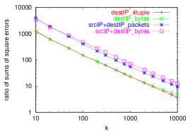
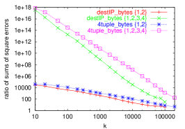
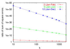
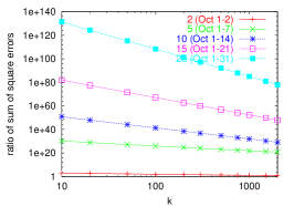
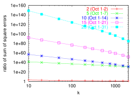
Figure 3: Top: IP dataset1 (left), IP dataset2 (middle), Netflix data set (right). Bottom: stocks dataset high values (left), stocks dataset volume values (middle). Ratio of $w^{(\min{\cal R})}$ estimators for independent and coordinated sketches ${\Sigma}V[a_{ind}^{(\min{\cal R})}]/{\Sigma}V[a_{\ell}^{(\min{\cal R})}]$.

Figure 3 shows the ratio ${\Sigma}V[a_{ind}^{(\min{\cal R})}]/{\Sigma}V[a_{\ell}^{(\min{\cal R})}]$ as a function of $k$ for our datasets. Across data sets, the variance of the independent-sketches estimator is significantly larger, up to many orders of magnitude, than the variance of coordinated-sketches estimators. The ratio decreases with $k$ but remains significant even when the sample size exceeds 10% of the number of keys.

The ratio increases with the number of weight assignments: On the Netflix data set, the ratio is 1-3 orders of magnitude for 2 months (assignments) and 10-40 orders of magnitude for 6-12 months (assignments). On IP dataset 2, the gap is 1-5 orders of magnitude for 2 assignments (hours) and 2-18 orders of magnitude for 4 assignments. On the stocks data set, the gap is 1-3 orders of magnitude for 2 assignments and reaches 150 orders of magnitude. This agrees with the exponential decrease of the inclusion probability with the number of assignments for independent sketches (see Section 7.2). These ratios demonstrate the estimation power provided by coordination.

Weighted versus unweighted coordinated sketches. We compare the performance of our estimators to known estimators applicable to unweighted coordinated sketches (coordinated sketches for uniform and global weights [18]). To apply these methods, all positive weights were replaced by unit weights. Because of the skewed nature of the weight distribution, the “unweighted” estimators performed poorly with variance being orders of magnitude larger.

Variance of multiple-assignment estimators. We relate the variance of our $w^{(\min{\cal R})}$, $w^{(\max{\cal R})}$, and $w^{(L_{1}{\cal R})}$ and the variance of the optimal single-assignment estimators $a^{(b)}$ for the respective individual weight assignments $w^{(b)}$ ($b\in{\cal R}$). Because the variance of $a_{ind}^{(\min{\cal R})}$ was typically many orders of magnitude worse, we include it only when it fit in the scale of the plot. The single-assignment estimators $a^{(b)}$ are identical for independent and coordinated sketches (constructed with the same $k$ and rank functions family), and hence are shown once.

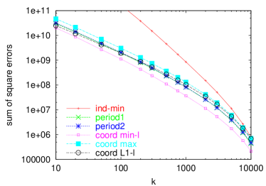
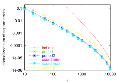
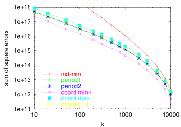
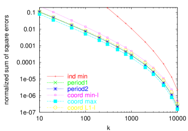
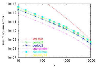
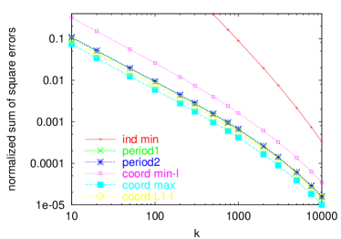
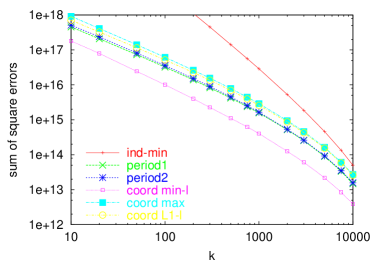
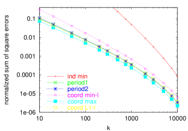
Figure 4: IP dataset1. Sum of square errors. left: absolute, right: normalized. Top: key$=$destIP weight$=$4tuple_count, second row: key$=$destIP weight$=$bytes. Third row: key$=$srcIP$+$destIP, weight$=$packets. Fourth row: key$=$srcIP$+$destIP, weight$=$bytes

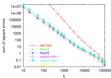
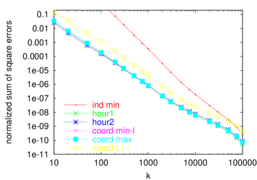
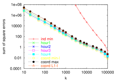
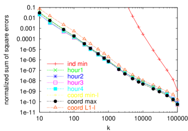
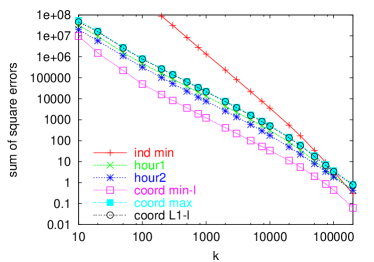
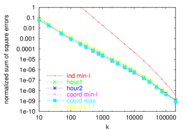
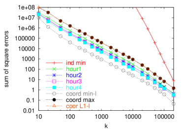
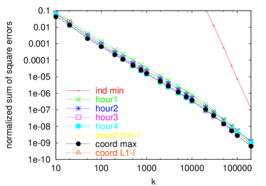
Figure 5: IP dataset2, sum of square errors. Left: absolute, Right: normalized. Top to bottom: key$=$destIP weight$=$bytes hours$=\{1,2\}$; key$=$destIP weight$=$bytes hours$=\{1,2,3,4\}$; key$=$4tuple weight$=$bytes hours$=\{1,2\}$; key$=$4tuple weight$=$bytes hours$=\{1,2,3,4\}$.

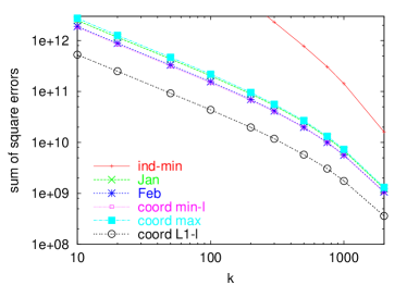
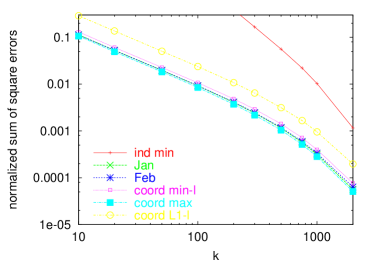
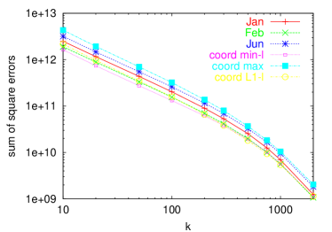
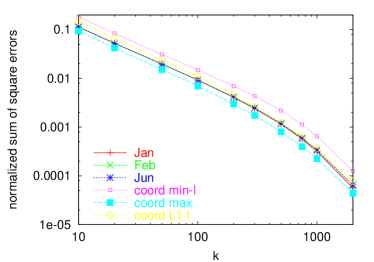
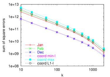
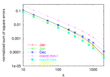
Figure 6: Netflix data set ${\cal R}=\{1,2\}$ (top), ${\cal R}=\{1,\ldots,6\}$ (middle), ${\cal R}=\{1,\ldots,12\}$ (bottom). ${\Sigma}V$ (left) and $n{\Sigma}V$ (right).

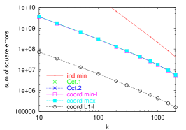
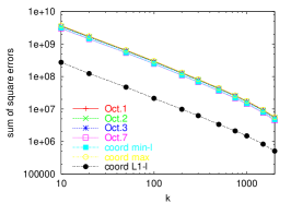
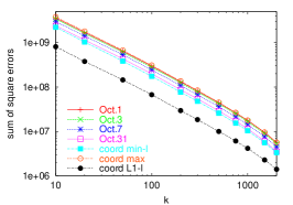
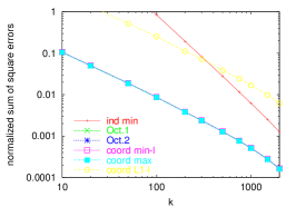
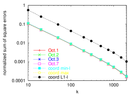
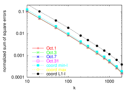
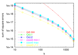
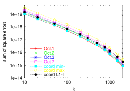
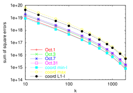
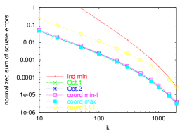
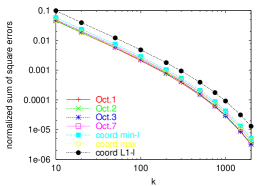
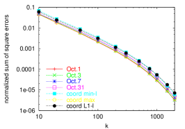
Figure 7: Stock dataset. Left: ${\cal R}=\{1,2\}$ (October 1-2, 2008), Middle: ${\cal R}=\{1,\ldots,5\}$ (trading days in October 1-7, 2008), Right: ${\cal R}=\{1,\ldots,23\}$ (all trading days in October, 2008). Upper two rows are ${\Sigma}V$ and $n{\Sigma}V$ with “high” weights. lower two rows are “volume” weights.

Figures 4, 5, 6 and 7 show, ${\Sigma}V[a_{\ell}^{(\min{\cal R})}]$, ${\Sigma}V[a_{\ell}^{(\max{\cal R})}]$, and ${\Sigma}V[a_{\ell}^{(L_{1}{\cal R})}]$ and ${\Sigma}V[a^{(b)}]$ for $b\in{\cal R}$ are within an order of magnitude. On our datasets, $n{\Sigma}V[a^{(b)}]$ and $n{\Sigma}V[a_{\ell}^{(\max{\cal R})}]$ are clustered together with $kn{\Sigma}V\ll 1$ (and decreases with $k$) (theory says $(k-2)n{\Sigma}V\leq 1$.) We also observed that $n{\Sigma}V[a_{l}^{(L_{1}{\cal R})}]$ and $n{\Sigma}V[a_{l}^{(\min{\cal R})}]$ are typically close to $n{\Sigma}V[a^{(b)}]$. We observe the empirical relations ${\Sigma}V[a_{\ell}^{(\min{\cal R})}]<{\Sigma}V[a_{\ell}^{(\max{\cal R})}]$ (with larger gap when the $L_{1}$ difference is very small), ${\Sigma}V[a_{\ell}^{(L_{1}{\cal R})}]<{\Sigma}V[a_{\ell}^{(\max{\cal R})}]$, and ${\Sigma}V[a_{\ell}^{(\min{\cal R})}]<\min_{b\in{\cal R}}{\Sigma}V[a^{(b)}]$. Empirically, the variance of our multi-assignment estimators with respect to single-assignment weights is significantly lower than the worst-case analytic bounds in Section 8 (Lemma 8.5 and 8.6). For normalized (relative) variances, we observe the “reversed” relations $n{\Sigma}V[a_{\ell}^{(\min{\cal R})}]>n{\Sigma}V[a_{\ell}^{(\max{\cal R})}]$, $n{\Sigma}V[a_{\ell}^{(L_{1}{\cal R})}]>n{\Sigma}V[a_{\ell}^{(\max{\cal R})}]$, and $n{\Sigma}V[a_{\ell}^{(\min{\cal R})}]>\max_{b\in{\cal R}}n{\Sigma}V[a^{(b)}]$ which are explained by smaller normalization factors for $w^{(\min{\cal R})}$ and $w^{(L_{1}{\cal R})}$.

S-set versus L-set estimators. Figure 8 quantifies the advantage of the stronger l-set estimators over the s-set estimators for coordinated sketches. The advantage highly varies between datasets: 15%-80% for the Netflix dataset, 0%-9% for IP dataset1, 0%-20% for IP dataset2, and 0%-300% on the Stocks data set.

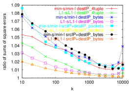
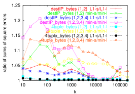
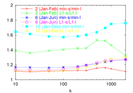
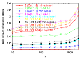
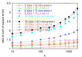
Figure 8: Top: IP dataset1 (left), IP dataset2 (middle), Netflix data set (right). Bottom: stocks dataset high-values (left), stocks dataset volume values (middle). ${\Sigma}V$ ratio of s-set and l-set estimators for $w^{(\min{\cal R})}$ and $w^{(L_{1}{\cal R})}$, ${\Sigma}V[a_{s}^{(\min{\cal R})}]/{\Sigma}V[a_{l}^{(\min{\cal R})}]$ and ${\Sigma}V[a_{s}^{(L_{1}{\cal R})}]/{\Sigma}V[a_{l}^{(L_{1}{\cal R})}]$.

9.3 Colocated data

We computed shared-seed coordinated and independent sketches and show results for ipps ranks (see Section 3). Results for exp ranks were similar.

We consider the following $w^{(b)}$-weights estimators. $a_{c}^{(b)}$: the shared-seed coordinated sketches inclusive estimator (Section 6, Eq. (6)). $a_{i}^{(b)}$: the independent sketches inclusive estimator in (Section 6, Eq. (5)). $a_{p}^{(b)}$: the plain bottom-$k$ sketch RC estimator ([26] for ipps ranks). Among all keys of the combined sketch this estimator uses only the keys which are part of the bottom-$k$ sketch of $b$.

We study the benefit of our inclusive estimators by comparing them to plain estimators. Since plain estimators can not be used effectively for multiple assignment aggregates, we focus on single-assignment aggregates.

Inclusive versus plain estimators. The plain estimators we used are optimal for individual bottom-$k$ sketches and the benefit of inclusive estimators comes from utilizing keys that were sampled for “other” weight assignments. We computed the ratios

$${\Sigma}V[a_{i}^{(b)}]/{\Sigma}V[a_{p}^{(b)}]\;\mbox{and}\;{\Sigma}V[a_{c}^{(b)}]/{\Sigma}V[a_{p}^{(b)}]$$

as a function of $k$. As Figures 9, 10 and 11 show, the ratios vary between 0.05 to 0.9 on our datasets and shows a significant benefit for inclusive estimators Our inclusive estimators are considerably more accurate with both coordinated and independent sketches. With independent sketches the benefit of the inclusive estimators is larger than with coordinate sketches since the independent sketches contain many more distinct keys for a given $k$.

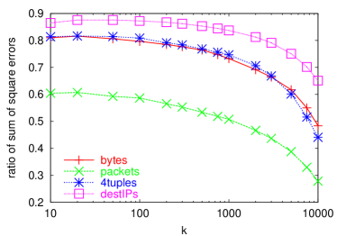
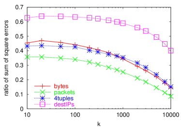
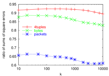
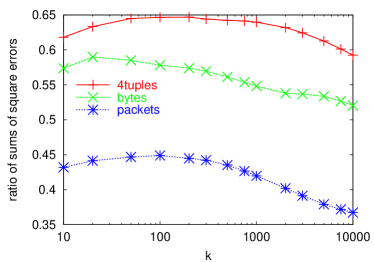
Figure 9: IP dataset1: Top: key$=$destIP. Bottom: key$=$4tuple. Left: ${\Sigma}V[a_{c}^{(b)}]/{\Sigma}V[a_{p}^{(b)}]$. Right: ${\Sigma}V[a_{i}^{(b)}]/{\Sigma}V[a_{p}^{(b)}]$.

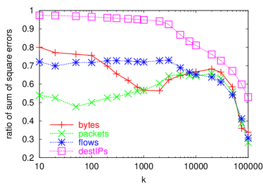
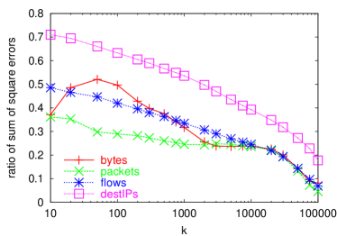
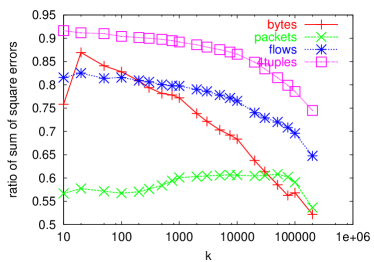
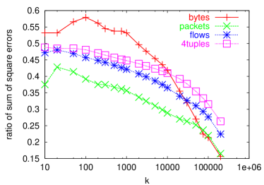
Figure 10: IP dataset2: Top: key$=$destIP. Bottom: key$=$4tuple. Left: ${\Sigma}V[a_{c}^{(b)}]/{\Sigma}V[a_{p}^{(b)}]$. Right: ${\Sigma}V[a_{i}^{(b)}]/{\Sigma}V[a_{p}^{(b)}]$.

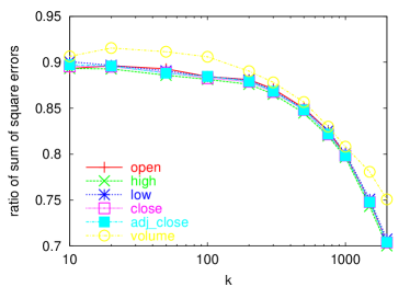
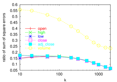
Figure 11: Stocks dataset: October 1, 2008. Left: ${\Sigma}V[a_{c}^{(b)}]/{\Sigma}V[a_{p}^{(b)}]$. Right: ${\Sigma}V[a_{i}^{(b)}]/{\Sigma}V[a_{p}^{(b)}]$.

Variance versus storage. For a fixed $k$, the plain estimator is in fact identical for independent and coordinated bottom-$k$ sketches. Independent bottom-$k$ sketches, however, tend to be larger than coordinated bottom-$k$ sketches. Here we compare the performance relative to the combined sample size, which is the number of distinct keys in the combined sample. We therefore use the notation $a_{p,i}^{(b)}$ for the plain estimator applied to independent sketches and $a_{p,c}^{(b)}$ for the plain estimator applied to coordinated sketches.

We compare summaries (coordinated and independent) and estimators (inclusive and plain) based on the tradeoff of variance versus summary size (number of distinct keys). Figures 12, 13, 14, and 15 show the normalized sums of variances, for inclusive and plain estimators $n{\Sigma}V[a_{i}^{(b)}]$, $n{\Sigma}V[a_{c}^{(b)}]$, $n{\Sigma}V_{p,c}[a^{(b)}]$, $n{\Sigma}V[a_{p,i}^{(b)}]$, as a function of the combined sample size. For a fixed sketch size, plain estimators perform worse for independent sketches than for coordinated sketches. This happens since an independent sketch of some fixed size contains a smaller sketch for each weight assignment than a coordinated sketch of the same size. In other words the “k” which we use to get an independent sketch of some fixed size is smaller than the “k” which we use to get a coordinated sketch of the same size. Inclusive estimators for independent and coordinated sketches of the same size had similar variance. (Note however that for a given union size, we get weaker confidence bounds with independent samples than with coordinated samples, simply because we are guaranteed fewer samples with respect to each particular assignment.)

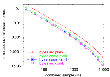
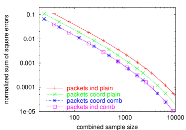
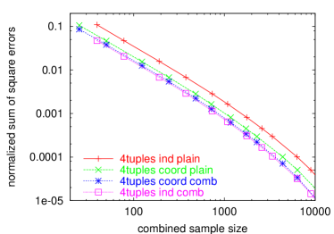
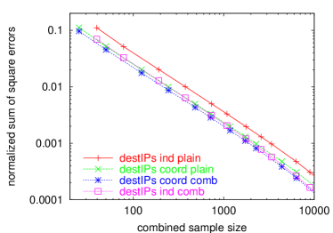
bytes packets 4tuples destIP

Figure 12: IP dataset1: key$=$destIP. $n{\Sigma}V[a_{i}^{(b)}]$, $n{\Sigma}V[a_{c}^{(b)}]$, $n{\Sigma}V[a_{p,i}^{(b)}]$, $n{\Sigma}V[a_{p,c}^{(b)}]$ as a function of (combined) sample size.

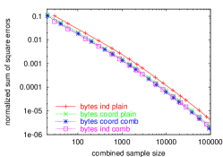
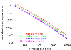
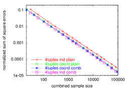
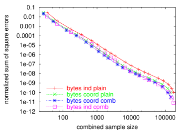
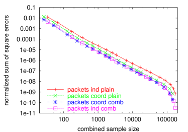
bytes packets 4tuples

Figure 13: IP dataset1: key$=$4tuples. $n{\Sigma}V[a_{i}^{(b)}]$, $n{\Sigma}V[a_{c}^{(b)}]$, $n{\Sigma}V[a_{p,i}^{(b)}]$, $n{\Sigma}V[a_{p,c}^{(b)}]$ as a function of (combined) sample size.

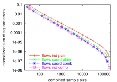
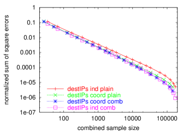
bytes packets 4tuples destIP

Figure 14: IP dataset2: key$=$destIP hour3. $n{\Sigma}V[a_{i}^{(b)}]$, $n{\Sigma}V[a_{c}^{(b)}]$, $n{\Sigma}V[a_{p,i}^{(b)}]$, $n{\Sigma}V[a_{p,c}^{(b)}]$ as a function of (combined) sample size.

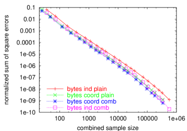
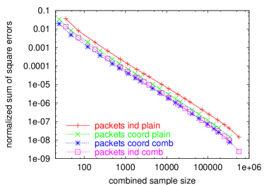
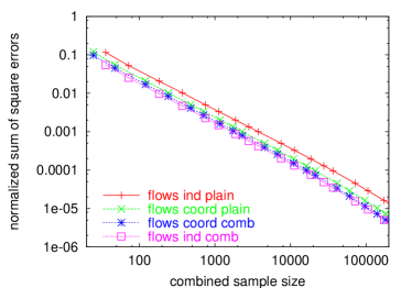
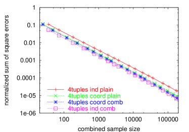
bytes packets flows 4tuples

Figure 15: IP dataset2: key$=$4tuple hour3. $n{\Sigma}V[a_{i}^{(b)}]$, $n{\Sigma}V[a_{c}^{(b)}]$, $n{\Sigma}V[a_{p,i}^{(b)}]$, $n{\Sigma}V[a_{p,c}^{(b)}]$ as a function of (combined) sample size.

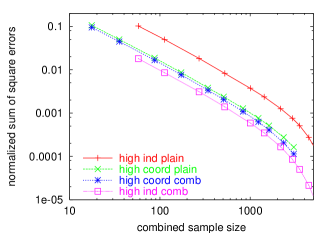
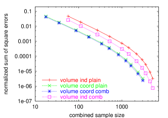
high volume

Figure 16: Stocks dataset. $n{\Sigma}V[a_{i}^{(b)}]$, $n{\Sigma}V[a_{c}^{(b)}]$, $n{\Sigma}V[a_{p,i}^{(b)}]$, $n{\Sigma}V[a_{p,c}^{(b)}]$ as a function of (combined) sample size.

Sharing index. The sharing index, $|S|/(k*|{\cal W}|)$ of a colocated summary $S$ is the ratio of the expected number of distinct keys in $S$ and the product of $k$ and the number of weight assignments $|{\cal W}|$. The sharing index falls in the interval $[1/|{\cal W}|,1]$ and is lower (better) when more keys are shared between samples of different assignments. More keys are shared when coordination is used and when weight assignments are more similar – when all assignments are identical and coordinated sketches are used then the index is exactly $1/|{\cal W}|$.

Figure 17 plots the sharing index for coordinated and independent bottom-$k$ sketches, as a function of $k$ for different data sets. Coordinated sketches minimize the sharing index (Theorem 4.2). On our datasets, the index lies in $[0.25,0.68]$ for coordinated sketches and in $[0.4,1]$ for independent sketches. The sharing index decreases when $k$ becomes a larger fraction of keys, both for independent and coordinated sketches – simply because it is more likely that a key is included in a sample of another assignment. For independent sketches, the sharing index is above $0.85$ for smaller values of $k$ and can be considerably higher than with coordinated sketches.

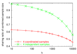
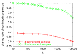
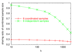
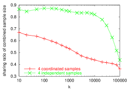
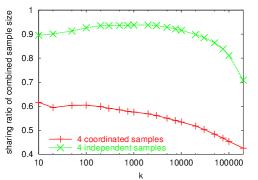
Figure 17: Sharing index of coordinated and independent sketches. Left: IP dataset1, key$=$destIP (4 weight assignments: bytes, packets, 4tuples, IPdests). Middle: IP dataset1, key$=$4tuple (3 weight assignments: bytes, packets, 4tuples). Right: Stocks dataset (6 weight assignments). Bottom: IP dataset2, key$=$destIP (left) IP dataset2, key$=$4tuple (middle)

10 Conclusion

We motivate and study the problem of summarizing data sets modeled as keys with vector weights. We identify two models for these data sets, dispersed (such as measurements from different times or locations) and collocated (records with multiple numeric attributes), that differ in the constraints they impose on scalable summarization. We then develop a sampling framework and accurate estimators for common aggregates, including aggregations over subpopulations that are specified a posteriori.

Our estimators over coordinated weighted samples for single-assignment and multiple-assignment aggregates including weighted sums and the $L_{1}$ difference, max, and min improve over previous methods by orders of magnitude. Previous methods include independent weighted samples from each assignment, which poorly supports multiple-assignment aggregates, and coordinated samples for uniform weights (each item has the same weight in all assignments where its weight is nonzero), which perform poorly when, as is often the case, weight values are skewed. For colocated data sets, our coordinated weighted samples achieve optimal summary size while guaranteeing embedded weighted samples of certain sizes with respect to each individual assignment. We derive estimators for single-assignment and multiple-assignment aggregates over both independent or coordinated samples that are significantly tighter than existing ones.

As part of ongoing work, we are applying our sampling and estimation framework to the challenging problem of detection of network problems. We are also exploring the system aspects of deploying our approach within the network monitoring infrastructure in a large ISP.

References

- [1] N. Alon, N. Duffield, M. Thorup, and C. Lund. Estimating arbitrary subset sums with few probes. In Proceedings of the 24th ACM Symposium on Principles of Database Systems, pages 317–325, 2005.
- [2] N. Alon, Y. Matias, and M. Szegedy. The space complexity of approximating the frequency moments. J. Comput. System Sci., 58:137–147, 1999.
- [3] K. S. Beyer, P. J. Haas, B. Reinwald, Y. Sismanis, and R. Gemulla. On synopses for distinct-value estimation under multiset operations. In SIGMOD, pages 199–210. ACM, 2007.
- [4] B. Bloom. Space/time tradeoffs in in hash coding with allowable errors. Communications of the ACM, 13:422–426, 1970.
- [5] K. R. W. Brewer, L. J. Early, and S. F. Joyce. Selecting several samples from a single population. Australian Journal of Statistics, 14(3):231–239, 1972.
- [6] A. Z. Broder. On the resemblance and containment of documents. In Proceedings of the Compression and Complexity of Sequences, pages 21–29. ACM, 1997.
- [7] A. Z. Broder. Identifying and filtering near-duplicate documents. In Proceedings of the 11th Annual Symposium on Combinatorial Pattern Matching, volume 1848 of LLNCS, pages 1–10. Springer, 2000.
- [8] M. T. Chao. A general purpose unequal probability sampling plan. Biometrika, 69(3):653–656, 1982.
- [9] M. S. Charikar. Similarity estimation techniques from rounding algorithms. In Proc. 34th Annual ACM Symposium on Theory of Computing. ACM, 2002.
- [10] A. Chowdhury, O. Frieder, D. Grossman, and M. C. McCabe. Collection statistics for fast duplicate document detection. ACM Transactions on Information Systems, 20(1):171–191, 2002.
- [11] E. Cohen. Size-estimation framework with applications to transitive closure and reachability. J. Comput. System Sci., 55:441–453, 1997.
- [12] E. Cohen, N. Duffield, H. Kaplan, C. Lund, and M. Thorup. Algorithms and estimators for accurate summarization of Internet traffic. In Proceedings of the 7th ACM SIGCOMM conference on Internet measurement (IMC), 2007.
- [13] E. Cohen, N. Duffield, H. Kaplan, C. Lund, and M. Thorup. Sketching unaggregated data streams for subpopulation-size queries. In Proc. of the 2007 ACM Symp. on Principles of Database Systems (PODS 2007). ACM, 2007.
- [14] E. Cohen, N. Duffield, H. Kaplan, C. Lund, and M. Thorup. Stream sampling for variance-optimal estimation of subset sums. In Proc. 20th ACM-SIAM Symposium on Discrete Algorithms. ACM-SIAM, 2009.
- [15] E. Cohen and H. Kaplan. Spatially-decaying aggregation over a network: model and algorithms. J. Comput. System Sci., 73:265–288, 2007.
- [16] E. Cohen and H. Kaplan. Summarizing data using bottom-k sketches. In Proceedings of the ACM PODC’07 Conference, 2007.
- [17] E. Cohen and H. Kaplan. Tighter estimation using bottom-k sketches. In Proceedings of the 34th VLDB Conference, 2008.
- [18] E. Cohen and H. Kaplan. Leveraging discarded samples for tighter estimation of multiple-set aggregates. In Proceedings of the ACM SIGMETRICS’09 Conference, 2009.
- [19] E. Cohen, H. Kaplan, and S. Sen. Coordinated weighted sampling for estimating aggregates over multiple weight assignments. Proceedings of the VLDB Endowment, 2(1–2), 2009.
- [20] J. G. Conrad and C. P. Schriber. Constructing a text corpus for inexact duplicate detection. In SIGIR 2004, pages 582–583, 2004.
- [21] G. Cormode and S. Muthukrishnan. Estimating dominance norms of multiple data streams. In Proceedings of the 11th European Symposium on Algorithms, pages 148–161. Springer-Verlag, 2003.
- [22] G. Cormode and S. Muthukrishnan. What’s new: finding significant differences in network data streams. IEEE/ACM Transactions on Networking, 13(6):1219–1232, 2005.
- [23] D. Crandall, D. Cosley, D. Huttenlocher, J. Kleinberg, and S. Suri. Feedback effects between similarity and social influence in online communities. In KDD’08. ACM, 2008.
- [24] T. Dasu, T. Johnson, S. Muthukrishnan, and V. Shkapenyuk. Mining database structure; or, how to build a data quality browser. In Proc. SIGMOD Conference, pages 240–251, 2002.
- [25] N. Duffield, C. Lund, and M. Thorup. Estimating flow distributions from sampled flow statistics. In Proceedings of the ACM SIGCOMM’03 Conference, pages 325–336, 2003.
- [26] N. Duffield, M. Thorup, and C. Lund. Priority sampling for estimating arbitrary subset sums. J. Assoc. Comput. Mach., 54(6), 2007.
- [27] P. S. Efraimidis and P. G. Spirakis. Weighted random sampling with a reservoir. Inf. Process. Lett., 97(5):181–185, 2006.
- [28] L. Fan, P. Cao, J. Almeida, and A. Z. Broder. Summary cache: a scalable wide-area Web cache sharing protocol. IEEE/ACM Transactions on Networking, 8(3):281–293, 2000.
- [29] J. Feigenbaum, S. Kannan, M. Strauss, and M. Viswanathan. An approximate L1-difference algorithm for massive data streams. In Proc. 40th IEEE Annual Symposium on Foundations of Computer Science, pages 501–511. IEEE, 1999.
- [30] P. Gibbons and Y. Matias. New sampling-based summary statistics for improving approximate query answers. In SIGMOD. ACM, 1998.
- [31] P. Gibbons and S. Tirthapura. Estimating simple functions on the union of data streams. In Proceedings of the 13th Annual ACM Symposium on Parallel Algorithms and Architectures. ACM, 2001.
- [32] P. B. Gibbons. Distinct sampling for highly-accurate answers to distinct values queries and event reports. In International Conference on Very Large Databases (VLDB), pages 541–550, 2001.
- [33] M. Hadjieleftheriou, X. Yu, N. Koudas, and D. Srivastava. Hashed samples: Selectivity estimators for set similarity selection queries. In Proceedings of the 34th VLDB Conference, 2008.
- [34] J. Hájek. Sampling from a finite population. Marcel Dekker, New York, 1981.
- [35] D. G. Horvitz and D. J. Thompson. A generalization of sampling without replacement from a finite universe. Journal of the American Statistical Association, 47(260):663–685, 1952.
- [36] D.E. Knuth. The Art of Computer Programming, Vol. 2: Seminumerical Algorithms. Addison-Wesley, 1969.
- [37] A. Kolcz, A. Chowdhury, and J. Alspector. Improved robustness of signature-based near-replica detection via lexicon randomization. In SIGKDD 2004, pages 605–610, 2004.
- [38] B. Krishnamurthy, S. Sen, Y. Zhang, and Y. Chen. Sketch-based change detection: Methods, evaluation, and applications. In In Internet Measurement Conference, pages 234–247. ACM Press, 2003.
- [39] A. Kumar, M. Sung, J. Xu, and E. W. Zegura. A data streaming algorithm for estimating subpopulation flow size distribution. ACM SIGMETRICS Performance Evaluation Review, 33, 2005.
- [40] G. Maier, R. Sommer, H. Dreger, A. Feldmann, V. Paxson, and F. Schneider. Enriching network security analysis with time travel. In SIGCOMM’ 08. ACM, 2008.
- [41] U. Manber. Finding similar files in a large file system. In Usenix Conference, pages 1–10, 1994.
- [42] G. S. Manku, A. Jain, and A. D. Sarma. Detecting nearduplicates for web crawling. In Proceedings of the 16th International World Wide Web Conference (WWW), 2007.
- [43] M. Mitzenmacher and S. Vadhan. Why simple hash functions work: exploiting the entropy in a data stream. In Proc. 19th ACM-SIAM Symposium on Discrete Algorithms, pages 746–755. ACM-SIAM, 2008.
-
[44]
The Netflix Prize.
http://www.netflixprize.com/. - [45] E. Ohlsson. Sequential poisson sampling. J. Official Statistics, 14(2):149–162, 1998.
- [46] E. Ohlsson. Coordination of pps samples over time. In The 2nd International Conference on Establishment Surveys, pages 255–264. American Statistical Association, 2000.
- [47] B. Rosén. Asymptotic theory for successive sampling with varying probabilities without replacement, I. The Annals of Mathematical Statistics, 43(2):373–397, 1972.
- [48] B. Rosén. Asymptotic theory for order sampling. J. Statistical Planning and Inference, 62(2):135–158, 1997.
- [49] F. Rusu and A. Dobra. Fast range-summable random variables for efficeint aggregate estimation. In Proc. of the 2006 ACM SIGMOD Int. Conference on Management of Data, pages 193–204. ACM, 1990.
- [50] P. J. Saavedra. Fixed sample size pps approximations with a permanent random number. In Proc. of the Section on Survey Research Methods, Alexandria VA, pages 697–700. American Statistical Association, 1995.
- [51] C-E. Särndal, B. Swensson, and J. Wretman. Model Assisted Survey Sampling. Springer, 1992.
- [52] S. Schleimer, D. Wilkerson, and A. Aiken. Winnowing: local algorithms for document fingerprinting. In Proceedings of the ACM SIGMOD, 2003.
- [53] R. Schweller, A. Gupta, E. Parsons, and Y. Chen. Reversible sketches for efficient and accurate change detection over network data streams. In in ACM SIGCOMM IMC, pages 207–212. ACM Press, 2004.
- [54] M. Szegedy. The DLT priority sampling is essentially optimal. In Proc. 38th Annual ACM Symposium on Theory of Computing. ACM, 2006.
- [55] M. Szegedy and M. Thorup. On the variance of subset sum estimation. In Proc. 15th ESA, 2007.
- [56] J.S. Vitter. Random sampling with a reservoir. ACM Trans. Math. Softw., 11(1):37–57, 1985.