Anomalous stabilization in a spin-transfer system at high spin polarization

Abstract

Switching diagrams of nanoscale ferromagnets driven by a spin-transfer torque are studied in the macrospin approximation. We consider a disk-shaped free layer with in-plane easy axis and external magnetic field directed in-plane at 90^∘ to that axis. It is shown that this configuration is sensitive to the angular dependence of the spin-transfer efficiency factor and can be used to experimentally distinguish between different forms of $g(\theta)$, in particular between the original Slonczewski form and the constant $g$ approximation. The difference in switching diagrams is especially pronounced at large spin polarizations, with the Slonczewski case exhibiting an anomalous region.

I Introduction

Spin polarized electric currents have been successfully used to switch the magnetization direction of nanoscale ferromagnetic layers via the spin transfer effect Sloczewski (1996); Berger (1996); Tsoi (1998); Myers (1999); Sun (1999); Katine (2000). One of the questions of current-induced dynamics is the dependence of spin-transfer efficiency, or Slonczewski factor $g$, on the angle between the polarization of incoming spin current and the magnetization direction Slonczewski (2002); Kovalev (2002); Xiao (2004); Zangwill (2005). Such a dependence can be essential, and for example leads to the asymmetry between the positive and negative switching currents. However, there is still a lack of experimental tests for the precise functional form of efficiency factor. It is expected that angular dependence of $g$ will become more important at high spin polarizations where the constant efficiency approximation can fail, while constant $g$ can still be in good agreement with experimental results at low spin polarization Wang (2006); Morise (2005); Yaroslaw (2007); Mancoff (2003).

Here we perform stability analysis for the equilibrium configurations of a bilayer spin-transfer device using the Slonczewski form for the efficiency factor and compare it with a similar analysis that uses the constant efficiency approximation. We observe that the switching diagram for the Slonczewski case displays a stability region and precessional states that are absent in the constant efficiency case. These anomalous regions become larger as the spin polarization increases. Our results may motivate further experimental efforts to directly measure the functional form of the efficiency factor at high spin polarizations.

II Macrospin description of the device

A typical device used to study spin-transfer effect is a nanopillar, with two layers of ferromagnetic material separated by a normal paramagnetic metal (see fig  1.a). The magnetization of one layer (polarizer) is fixed and oriented along a unit vector $\mathbf{s}$, while the magnetization of the other (free layer), $\mathbf{M}=M\mathbf{n}$, rotates and is described in the macrospin approximation by the Landau-Lifshitz-Gilbert (LLG) equation including the Slonczewski spin torque term Sloczewski (1996)

$$\mathbf{\dot{n}}=\frac{\gamma}{M}\Bigg{[}-\frac{\delta E}{\delta\mathbf{n}}\times\mathbf{n}\Bigg{]}+\frac{\gamma\hbar I}{2eVM}g(\theta,P)[\mathbf{n}\times(\mathbf{s}\times\mathbf{n})]+\alpha[\mathbf{n}\times\mathbf{\dot{n}}],$$ (1)

where $\gamma$ is the gyromagnetic ratio, $E(\mathbf{n})$ is the magnetic energy of the free layer, and $\alpha$ is the Gilbert damping constant. The strength of the spin-torque is characterized by the efficiency factor, $g(\theta,P)$, which depends on the angle $\theta$ between the magnetizations of the polarizer and the free layer, and the degree of current spin polarization $P\in[0,1]$. In general the functional form of $g(\theta,P)$ is material and geometry-dependent Slonczewski (2002); Kovalev (2002); Xiao (2004); Zangwill (2005). Here we will compare Slonczewski’s Sloczewski (1996) form

$$g(\theta,P)=\frac{1}{f_{P}(\xi_{P}+\cos\theta)},$$ (2)

with $\xi_{P}=3-4/f_{P}$, $f_{P}=(1+P)^{3}/4P^{3/2}$ and the $g(\theta,P)$=const approximation.

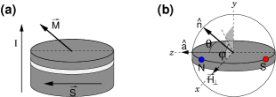
Figure 1: a) Typical nanopillar device with free layer on the top and polarizer at the bottom. b) In-plane magnetic field configuration. Two stable directions of the free layer magnetization are labeled as N and S.

The magnetic energy of the free layer includes contributions from the intrinsic anisotropy (easy axis anisotropy with strength $H_{a}$ and direction $\mathbf{\hat{a}}$), shape anisotropy (easy plane anisotropy with normal vector $\mathbf{\hat{p}}$) and the interaction energy with an external magnetic field $\mathbf{H}$. Equation (1) can be written as

$$\mathbf{\dot{n}}=\boldsymbol{\tau}(\mathbf{n})+\alpha\mathbf{n}\times\boldsymbol{\tau}(\mathbf{n})\ ,$$ (3)

where we have rescaled the time as $T=t/(1+\alpha^{2})$, and $\boldsymbol{\tau}$ is defined as

$$\boldsymbol{\tau}(\mathbf{n}) =-\nabla\varepsilon(\mathbf{n})\times\mathbf{n}+\omega_{I}g(\theta,P)\ \mathbf{n}\times(\mathbf{s}\times\mathbf{n}),$$ (4)

$$\varepsilon(\mathbf{n}) =\frac{\omega_{p}}{2}(\mathbf{\hat{p}\cdot\mathbf{n}})^{2}-\frac{\omega_{a}}{2}(\mathbf{\hat{a}\cdot\mathbf{n}})^{2}-\omega_{H}(\mathbf{\hat{h}}\cdot\mathbf{n}).$$

The newly defined constants are related to the already introduced parameters according to

$$\omega_{a} =\gamma H_{a}, \omega_{p} =4\pi\gamma M,$$ (5)

$$\omega_{H} =\gamma H, \omega_{I} =\frac{\gamma\hbar}{2eVM}I.$$

All of them have dimensions of frequency making the comparison between the terms of different origin straightforward. In accord with experimental situations it is assumed that $\omega_{I}\ll\omega_{p}$.

We study a device with an in-plane easy axis and the in-plane magnetic field perpendicular to it (see fig. 1.b). Choosing the system of coordinates $\mathbf{\hat{s}}=\mathbf{\hat{a}}=\mathbf{\hat{e}_{z}}$, $\mathbf{\hat{h}}=\mathbf{\hat{e}_{x}}$, $\mathbf{\hat{p}}=\mathbf{\hat{e}_{y}}$, we obtain, from equation (4), the components of $\boldsymbol{\tau}$ in spherical coordinates

$$\begin{split}\tau_{\phi}&=\frac{1}{2}\sin 2\theta(\omega_{p}\sin^{2}\phi+\omega_{a})-\omega_{H}\cos\theta\cos\phi,\\ \tau_{\theta}=&-\frac{\omega_{p}}{2}\sin\theta\sin 2\phi-\omega_{H}\sin\phi-\omega_{I}g(\cos\theta)\sin\theta.\end{split}$$ (6)

The equilibrium directions of the magnetization $\bf n$ correspond to the solutions of the equation $\boldsymbol{\tau}(\mathbf{n})=0$. Here we consider the two in-plane equilibrium points. At $\omega_{I}=0$, $\omega_{H}=0$ these are the north (N) and the south (S) poles. For $\omega_{I}=0$, $\omega_{H}\neq 0$ they shift and approach the direction of magnetic field, finally merging at $\omega_{H}=\omega_{a}$. The shifted equilibrium points are still labeled by N and S (Fig. 1b).

Stability of an equilibrium can be checked by expanding $\mathbf{\tau}$ in angular deviations $\delta\theta$, $\delta\phi$, and writing equation (3) in an approximate form

$$\dbinom{\dot{\phi}}{\dot{\theta}}=\mathbf{D}\dbinom{\delta\phi}{\delta\theta}.$$ (7)

The equilibrium is stable when the real parts of both eigenvalues of $\mathbf{D}$ are negative, or equivalently when matrix $\bf D$ satisfies ${\rm Tr}\mathbf{D}<0$ and ${\det}\mathbf{D}>0$ at the equilibrium.

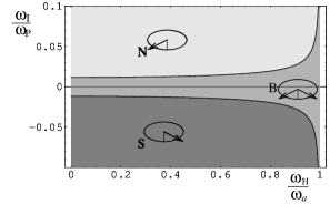
Figure 2: Switching diagram for the $g=$const approximation. The value of $g$ is chosen as the average value of Slonczewski’s $g(\theta)$ used in Fig. 3. Other parameters are set to $\omega_{a}/\omega_{p}=0.01$, $P=0.7$, and $\alpha=0.01$. Stability regions for the N and S equilibria (see text) overlap forming the bistable region marked as B.

III Stability regions

The modified positions of the N and S equilibria for $\omega_{H}\neq 0$, $\omega_{I}\neq 0$ are given by

$$\begin{split}\sin\theta_{N,S}&=\frac{\omega_{H}}{\omega_{a}}+\mathcal{O}\left(\frac{\omega_{I}}{\omega_{P}}\right)^{2},\\ \sin\phi_{N,S}=-&g_{N,S}\frac{\omega_{I}}{\omega_{p}}\left(1+\frac{\omega_{a}}{\omega_{p}}\right)+\mathcal{O}\left(\frac{\omega_{I}}{\omega_{P}}\right)^{2},\end{split}$$ (8)

for $0<\omega_{H}<\omega_{a}$ (with $g_{N,S}=g(\theta_{N,S})$). The angle $\theta$ and the magnetic field strength $\omega_{H}$ have a one-to-one correspondence and can be used interchangeably. The trace of $\mathbf{D}$-matrix at these points can be found as

$$\begin{split}\rm Tr\mathbf{D}=&-\omega_{I}\left[g(\theta)\cos\theta+\frac{d}{d\theta}(g(\theta)\sin\theta)\right]\\ &-\alpha[\omega_{p}\cos 2\phi+(\omega_{p}\sin^{2}\phi+\omega_{a})(1+\cos^{2}\theta)]\end{split}$$ (9)

Approximations (8) give the stability condition in the form

$$\begin{split}\alpha\left[1+\frac{\omega_{a}}{\omega_{p}}(1+\cos^{2}\theta)\right]>-&\frac{\omega_{I}}{\omega_{p}}\left[2g(\theta)\cos\theta+g^{\prime}(\theta)\sin\theta\right]\\ &+\mathcal{O}\left(\frac{\omega_{I}}{\omega_{P}}\right)^{2}.\end{split}$$ (10)

The determinant

$$\frac{1}{1+\alpha^{2}}\det\mathbf{D}=\omega_{a}(\omega_{p}+\omega_{a})\cos^{2}\theta+\mathcal{O}(\omega_{I}^{2}),$$ (11)

in the small current regime remains positive, so it does not play any role in the stability analysis in this case. In contrast, the trace ${\rm Tr}\mathbf{D}$ is more sensitive and can change sign as the current is varied. Moreover, the explicit appearance of $g^{\prime}(\theta)$ in the formula leads to important differences in the switching diagrams for different forms of $g(\theta)$. In the case of constant $g$-factor the stability condition for N- and S-equilibira can be written as

$$\omega_{I}\gtrless\mp\alpha\frac{\omega_{p}+\omega_{a}(2-(\omega_{H}/\omega_{a})^{2})}{2g\sqrt{1-(\omega_{H}/\omega_{a})^{2}}}$$ (12)

where $>$, $-$ ($<$, $+$) corresponds to the N (S) stability region (See Fig. 2). The switching current exhibits the $1/\cos\theta$ divergence reported in the experiments for this regime Mancoff (2003).

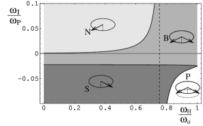
Figure 3: Switching diagrams for the Slonczewski’s form of $g$-factor. Other parameters are the same as in Fig. 2. Regions of stability for north (N) and south (S) poles overlapping in the bistable region (B), and the region of precessional states (P) are shown. The onset of the anomalous stability behavior occurs at a field $\omega^{*}_{H}/\omega_{P}=0.76$.

For the Slonczewski $g$-factor, the condition of stability for the N point is

$$\omega_{I}>-\alpha\frac{\omega_{p}+\omega_{a}(2-(\omega_{H}/\omega_{a})^{2})}{2g_{N}\sqrt{1-(\omega_{H}/\omega_{a})^{2}}+g^{2}_{N}f_{P}(\omega_{H}/\omega_{a})^{2}},$$ (13)

whereas for the S point the condition becomes

$$\omega_{I}\lessgtr\alpha\frac{\omega_{p}+\omega_{a}(2-(\omega_{H}/\omega_{a})^{2})}{2g_{S}\sqrt{1-(\omega_{H}/\omega_{a})^{2}}-g^{2}_{S}f_{P}(\omega_{H}/\omega_{a})^{2}},$$ (14)

where $<$ ($>$) is the condition for $\omega<\omega^{*}_{H}$ ($\omega>\omega^{*}_{H}$), $\omega^{*}_{H}$ designates the field for which the denominator of equation (14) becomes zero, and determines the onset of an stability behavior completely absent in the $g$-constant case (Fig. 3). This field, or equivalently the angle characterizing the S point, depends only on polarization $P$ and can be found from

$$\cos\theta_{c}=-\sqrt{1-(\omega_{H}^{*}/\omega_{a})^{2}}=\sqrt{\xi^{2}_{P}-1}-\xi_{P}.$$ (15)

In the “anomalous” regime $\omega_{H}>\omega_{H}^{*}$ a current of positive polarity stabilizes both N and S points, while the application of a sufficiently large negative current destabilizes both points (see Fig. 3), moreover, there is a region in which none of the equilibria are stable, suggesting the existence of precessional motion. The value of $\omega^{*}_{H}$ becomes smaller as the polarization increases. In the limit $P\rightarrow 1$ it becomes zero, so that the anomalous region fills all the switching diagram. In other words, as the polarization becomes larger the differences between the $g$-constant approximation and the Slonczewski form become quite dramatic. The position $\theta_{c}$ of the S point at $\omega_{H}^{*}$ is shown in Fig. 4.

Figure 4: Critical angle $\theta_{c}$ for the onset of the anomalous stabilization as function of the polarization

Substantial difference between the switching diagrams at large spin polarizations found in this study underscores the necessity of developing new experiments capable of determining the $g(\theta)$ dependence. It also suggests that in the regime of large spin polarization the behavior of spin-transfer devices may experience qualitative changes.