Expansive homeomorphisms of the plane.

Abstract

This article tackles the problem of the classification of expansive homeomorphisms of the plane. Necessary and sufficient conditions for a homeomorphism to be conjugate to a linear hyperbolic automorphism will be presented. The techniques involve topological and metric aspects of the plane. The use of a Lyapunov metric function which defines the same topology as the one induced by the usual metric but that, in general, is not equivalent to it is an example of such techniques. The discovery of a hypothesis about the behavior of Lyapunov functions at infinity allows us to generalize some results that are valid in the compact context. Additional local properties allow us to obtain another classification theorem.

IMERL, Facultad de Ingeniería, Universidad de la República, Montevideo Uruguay
(e-mail: jorgeg@fing.edu.uy)

1 Introduction

The aim of this work is to describe the set of expansive homeomorphisms of the plane with one fixed point under certain conditions. The original question that we asked ourselves was whether every expansive homeomorphism of the plane was a lift of an expansive homeomorphism on some compact surface. As it is well known, such expansive homeomorphisms were classified by Lewowicz in [7] and Hiraide in [5]. As a matter of fact, we began by studying whether some of the results obtained in the previously cited article could be adapted to our new context (i.e. without working in a compact environment but having the local compactness of the plane). In this work I study expansive homeomorphisms with one fixed point, singular or not, and without stable (unstable) points. The existence of a Lyapunov function that allows us, among other things, to generalize Lewowicz’s results on stable and unstable sets will be essential. In fact, it will also allow us to obtain a characterization of those homeomorphisms of the plane which are liftings of expansive homeomorphisms on $T^{2}$. The result can be tested in any given homeomorphism $f$ provided with a suitable Lyapunov function. Although many of the techniques used in this work are valid for the case where there are many singularities, we leave the study of this situation for forthcoming papers.
Let $f:I\kern-3.69995ptR^{2}\rightarrow I\kern-3.69995ptR^{2}$ be a homeomorphism of the plane that admits a Lyapunov metric function $U$, meaning $U:I\kern-3.69995ptR^{2}\times I\kern-3.69995ptR^{2}\rightarrow I\kern-3.69995ptR$ continuous and positive (i.e. it is equal to zero only on the diagonal) and $W=\Delta(\Delta U)$ positive with $\Delta U(x,y)=U(f(x),f(y))-U(x,y)$. We define $f$ as being $U$-expansive if given two different points of the plane $x,y$ the following property holds: for every $k>0$, there exists $n\in{\bf Z}$ such that

$$U(f^{n}(x),f^{n}(y))>k.$$

The main objective of this work is to describe every expansive homeomorphism $f$ with one fixed point where some Lyapunov metric function $U$ verifies certain conditions concerning $f$. During this work we will require the existence of such a Lyapunov function $U$, unlike in the compact case where expansiveness is a necessary and sufficient condition for the existence of a Lyapunov function (see [7] ). In the previous reference, Lewowicz classifies expansive homeomorphisms on compact surfaces. Our main results is (Theorem 4.2.1): A homeomorphism $f:I\kern-3.69995ptR^{2}\rightarrow I\kern-3.69995ptR^{2}$ with a fixed point is conjugate to a linear hyperbolic automorphism if and only if it admits a Lyapunov metric function that satisfies condition HP and it has not singular points. Condition HP establishes that: given any compact set $C$ of $I\kern-3.69995ptR^{2}$, the following property holds

$$\lim_{x\rightarrow\infty}\frac{|V(x,y)-V(x,z)|}{W(x,y)}=0,$$

uniformly with $y,z$ in $C$ and $V=\Delta U,W=\Delta V$.
Without condition HP and demanding other kind of conditions for $U$, different behaviors appear. These are described in Theorem 5.1.1: Let $f$ be a homeomorphism of the plane with a fixed point. $f$ admits a Lyapunov function $U$ that verifies hypothesis HL if and only if $f$ restricted to each quadrant determined by the stable and unstable curves of the fixed point is conjugated (such conjugations must preserve stable and unstable curves) either to a linear hyperbolic automorphism or to a restriction of a linear hyperbolic automorphism to certain invariant region. The most important part of condition HL establishes that:

• the first difference $V=\Delta U$ verifies the following property: given $\epsilon>0$ there exists $\delta>0$ such that if $U(z,y)<\delta$ then $|V(x,z)-V(x,y)|<\epsilon$, $\forall x\in I\kern-3.69995ptR^{2}$;

• the second difference $W=\Delta^{2}U$ verifies the following property: given $\delta>0$, there exists $a(\delta)>0$ such that $W(x,y)>a(\delta)>0$ for every $x,y$ on the plane with $U(x,y)>\delta$.

The difference between the two cases (presented in Theorem 5.1.1) consists of the existence of stable and unstable curves that do not intersect each other. In 5.2 we will show examples about the case where there are stable and unstable curves that do not intersect each other.
We also conjecture that if $f:I\kern-3.69995ptR^{2}\rightarrow I\kern-3.69995ptR^{2}$ is a preserving-orientation and fixed point free homeomorphism that admits a Lyapunov function $U:I\kern-3.69995ptR^{2}\times I\kern-3.69995ptR^{2}\rightarrow I\kern-3.69995ptR$ satisfying condition HP, then it must be topologically conjugate to a translation of the plane. We believe that the proof of this assertion is a consequence of Brouwer’s translation theorem (see [1], [3]) and of some techniques used in this article. We leave the study of this situation for forthcoming works.
Regarding the structure of the paper, we begin section 2 by studying some properties that are verified by a Lyapunov function associated to a lift of an expansive homeomorphism in the compact case, as well as to homeomorphisms conjugated to it. In section 3 we describe stable and unstable sets, by adapting Lewowicz’s arguments used on [7]. In Section 4 we show our main result. In Section 5 we study an other context and some examples.

2 Preliminaries

During the course of this work we will consider homeomorphisms of the plane which admit a Lyapunov metric function $U$ with certain characteristics. These properties are natural since they are verified by a Lyapunov function of a lift of an expansive homeomorphism in the compact case. In this section we will verify some of these properties. In [2], [9] is proved that every lift $F$ of an expansive homeomorphism on compact surfaces satisfies the existence of pseudo-metrics $D_{s}$, $D_{u}$ and $\lambda>1$ such that for every $\xi,\ \eta\in I\kern-3.69995ptR^{2}$ the following holds:

$$D_{s}(F^{-1}(\xi),F^{-1}(\eta))=\lambda D_{s}(\xi,\ \eta);$$

$$D_{u}(F(\xi),F(\eta))=\lambda D_{u}(\xi,\ \eta),$$

where $D=D_{s}+D_{u}$ is a Lyapunov metric in $I\kern-3.69995ptR^{2}$ for $F$.
We will test the following properties:

• Signs for $\Delta(D)$. We shall use the notation $B_{k}(x)$ for the connected component of set $B_{k}(x)=\{y\in I\kern-3.69995ptR^{2}\ /D(x,y)\leq k\}$, which contains $x$. For every point $x\in I\kern-3.69995ptR^{2}$ and for every $k>0$, there are points $y$ in the border of $B_{k}(x)$ such that $\Delta D(x,y)=D(f(x),f(y))-D(x,y)>0$ and points $z$ in the border of $B_{k}(x)$ such that $\Delta D(x,z)=D(f(x),f(z))-D(x,z)<0$. This property will be essential to describe stable and unstable sets.

• Property HP. Let $V=\Delta D$ and $W=\Delta^{2}D$. Given any compact set $C\subset I\kern-3.69995ptR^{2}$, the following property holds

  $$\lim_{\|x\|\rightarrow\infty}\frac{|V(x,y)-V(x,z)|}{W(x,y)}=0,$$

  uniformly with $y,z$ in $C$. This property will be essential to prove the main result on this work.

2.1 Lifted case.

Let $D=D_{s}+D_{u}$ be the Lyapunov metric function that we introduced at the beginning of this section.

• Signs for $\Delta D$. Proof:

  $$\Delta D(x,y)=D(f(x),f(y))-D(x,y)=$$

  $$D_{s}(f(x),f(y))-D_{s}(x,y)+D_{u}(f(x),f(y))-D_{u}(x,y)=$$

  $$(\lambda-1)D_{u}(x,y)-(1-1/\lambda)D_{s}(x,y).$$

  For every point $x\in I\kern-3.69995ptR^{2}$ and for every $k>0$, there are points $y$ in the border of $B_{k}(x)$ such that $D_{u}(x,y)=0$ (this is true because the stable set separates the plane). Therefore, $\Delta D(x,y)<0$ as we wanted. A similar argument lets us find points $z\in I\kern-3.69995ptR^{2}$ such that $\Delta D(x,z)>0$. $\Box$

• Property HP. Proof: Since

  $$\Delta^{2}D(x,y)=\Delta D(f(x),f(y))-\Delta D(x,y)=$$

  $$(\lambda-1)^{2}D_{u}(x,y)+(1-1/\lambda)^{2}D_{s}(x,y),$$

  we can conclude that $\Delta^{2}D(x,y)$ tends to infinity when $x$ tends to infinity. Now,

  $$|\Delta D(x,y)-\Delta D(x,z)|\leq$$

  $$(\lambda-1)|D_{u}(x,y)-D_{u}(x,z)|+(1-1/\lambda)|D_{s}(x,y)-D_{s}(x,z)|\leq$$

  $$(\lambda-1)D_{u}(z,y)+(1-1/\lambda)D_{s}(z,y).$$

  Then $|\Delta D(x,y)-\Delta D(x,z)|$ is uniformly bounded when points $y$ and $z$ lie on a compact set. Then property HP holds. $\Box$

2.2 Lifted conjugated case.

Now, let us start with the case where $f$ is conjugated to a lift $F$ of an expansive homeomorphism on a compact surface. Let us define a Lyapunov function for $f$ such as

$$L(p_{1},p_{2})=D(H(p_{1}),H(p_{2})),$$

where $D$ is the previous defined Lyapunov metric function for $F$ and $H$ is a homeomorphism from $I\kern-3.69995ptR^{2}$ over $I\kern-3.69995ptR^{2}$. It follows easily that $L$ is a Lyapunov function for $f$ and a metric in $I\kern-3.69995ptR^{2}$.

• Signs for $\Delta(L)$. Proof: It is clear since

  $$\Delta L(p_{1},p_{2})=\Delta D(H(p_{1}),H(p_{2})),$$

  and $H$ is continuous at infinity. $\Box$

• Property HP. Proof:

  $$|\Delta(L)(p,q)-\Delta(L)(p,r)|=$$

  $$|\Delta D(H(p),H(q))-\Delta D(H(p),H(r))|\leq$$

  $$(\lambda-1)D_{u}(H(q),H(r))+(1-1/\lambda)D_{s}(H(q),H(r))\leq K,$$

  since $q$ and $r$ are in a compact set and $H$ is a homeomorphism. Since

  $$\Delta^{2}(L)(p,q)=\Delta^{2}D(H(p),H(q))$$

  and $H$ is continuous at infinity we conclude that $\Delta^{2}(L)(p,q)$ tends to infinite when $p$ tends to infinity. Then, if $f$ is conjugated to a lift of an expansive homeomorphism on a compact surface, it admits a Lyapunov function $L$ such that condition (HP) holds. $\Box$

3 Stable and unstable sets.

In this section we will stay close to the arguments used by Lewowicz in [7], Sambarino in [8] and Groisman in [4]. We have to adapt them for our non-compact context. We will work with the topology induced by a Lyapunov function $U$ and define the $k$-stable set in the following way:

$$S_{k}(x)=\{y\in I\kern-3.69995ptR^{2}:\ U(f^{n}(x),f^{n}(y))\leq k,\forall n\in I\kern-3.69995ptN\}.$$

Similar definition for the $k$-unstable set $U_{k}$. Let $f$ be a homeomorphism of the plane that admits a Lyapunov function $U:I\kern-3.69995ptR^{2}\times I\kern-3.69995ptR^{2}\rightarrow I\kern-3.69995ptR$ such that the following properties hold:

• $U$ is a metric in $I\kern-3.69995ptR^{2}$ and induces the same topology in the plane as the usual metric. Observe that given any Lyapunov function it is possible to obtain another Lyapunov function that verifies all the properties of a metric except, perhaps, for the triangular property.

• Existence of both signs for the first difference of $U$. For each point $x\in I\kern-3.69995ptR^{2}$ and for each $k>0$ there exist points $y$ and $z$ on the border of $B_{k}(x)$ such that $V(x,y)=U(f(x),f(y))-U(x,y)>0$ and $V(x,z)=U(f(x),f(z))-U(x,z)<0$, respectively.

Remark 3.0.1

A homeomorphism $f$ that admits a Lyapunov function $U$ defined at $I\kern-3.69995ptR^{2}\times I\kern-3.69995ptR^{2}$ is U-expansive. This means that given two different points of the plane $x,y$ and given any $k>0$, there exists $n\in{\bf Z}$ such that

$$U(f^{n}(x),f^{n}(y))>k.$$

Proof: Let $x$ and $y$ be two different points of the plane such that $V(x,y)>0$. Since $\Delta V>0$, then $V(f^{n}(x),f^{n}(y))>V(x,y)$ holds for $n>0$. This means that $U(f^{n}(x),f^{n}(y))$ grows to infinity, since

$$U(f^{n}(x),f^{n}(y))=U(x,y)+\sum_{j=1}^{n}V(f^{j}(x),f^{j}(y))>$$

$$U(x,y)+nV(x,y).$$

Thus, given $k>0$ there exists $n\in I\kern-3.69995ptN$ such that

$$U(f^{n}(x),f^{n}(y))>k.$$

By using similar arguments we can prove the case when $V(x,y)=U(f(x),f(y))-U(x,y)<0$. If $V(x,y)=0$, then $V(f(x),f(y))>0$ and this is precisely our first case. $\Box$

Definition 3.0.1

Let $f:I\kern-3.69995ptR^{2}\rightarrow I\kern-3.69995ptR^{2}$ be a homeomorphism of the plane that admits a Lyapunov metric function $U$. A point $x\in I\kern-3.69995ptR^{2}$ is a stable (unstable) point if given any $k^{\prime}>0$ there exists $k>0$ such that for every $y\in B_{k}(x)$, it follows that $U(f^{n}(x),f^{n}(y))<k^{\prime}$ for each $n\geq 0$ ($n\leq 0$).

Remark 3.0.2

Property $(2)$ for $U$ implies the non-existence of stable (unstable) points.

Proof: Given the existence of both signs for $V(x,y)=U(f(x),f(y))-U(x,y)$ in any neighborhood of $x$, we can state that for each $k>0$, there exists a point $y$ in $B_{k}(x)$ such that $V(x,y)>0$. Since $\Delta V>0$, we can state that $V(f^{n}(x),f^{n}(y))>V(x,y)$ for $n>0$, so $U(f^{n}(x),f^{n}(y))$ grows to infinity. Thus, there are no stable points. We can use similar arguments for the unstable case. $\Box$

Remark 3.0.3

There does not exist $x,y\in I\kern-3.69995ptR^{2}$ and $n\in{\bf Z}$ such that

$$U(f^{n+1}(y),f^{n+1}(x))>U(f^{n}(y),f^{n}(x))$$

and

$$U(f^{n+1}(y),f^{n+1}(x))>U(f^{n+2}(y),f^{n+2}(x)).$$

Proof: Suppose that there exist two different points $x,y\in I\kern-3.69995ptR^{2}$ and $n\in I\kern-3.69995ptN$ such that they do not verify the thesis. Since

$$\triangle(\triangle U)(f^{n}(x),f^{n}(y))=$$

$$U(f^{n+2}(x),f^{n+2}(y))-2U(f^{n+1}(x),f^{n+1}(y))+U(f^{n}(x),f^{n}(y)),$$

we have that

$$\triangle(\triangle U)(f^{n}(x),f^{n}(y))<U(f^{n+1}(x),f^{n+1}(y))-2U(f^{n+1}(x),f^{n+1}(y))+$$

$$U(f^{n+1}(x),f^{n+1}(y))=0,$$

which is not possible. $\Box$

Lemma 3.0.1

Let $A$ be an open set of $I\kern-3.69995ptR^{2}$ with $x\in A\subset B_{k}(x)$. There exists a compact connected set $C$ with $x\in C\subset\overline{A}$, $C\cap\partial(A)\neq\emptyset$ such that, for all $y\in C$ and $n\geq 0$, $U(f^{n}(x),f^{n}(y))\leq k$ holds.

Proof: Suppose that there exists $N>0$ such that for each compact connected set $D\subset\overline{A}$ that joins $x$ with the border of $A$, there exists $z\in D$ and $n$ with $0\leq n\leq N$ such that $U(f^{n}(x),f^{n}(z))>k$. Otherwise, for each $n\geq 0$ we would find $D_{n}\subset\overline{A}$ that joins $x$ with the border of $A$ such that for every $y\in D_{n}$, $U(f^{m}(x),f^{m}(y))\leq k$, $0\leq m\leq n$. Then

$$D_{\infty}=\bigcap_{n=0}^{\infty}\overline{\left(\bigcup_{j=n}^{\infty}D_{j}\right)},$$

is a connected compact set that satisfies our assertion. Let us go back to the prior assumption. Consider a point $y$ in the border of $B_{k}(f^{n}(x))$ that belongs to the region where $V(f^{n}(x),y)=U(f^{n+1}(x),f(y))-U(f^{n}(x),y)<0$, this means that $U(f^{n+1}(x),f(y))<k$. Then $U(f^{n-1}(x),f^{-1}(y))>k$, because otherwise, we would contradict the previous remark. So, $\overline{B_{k}(f^{n}(x))}$ contains points $y$ such that $f^{-1}(y)$ does not belong to $\overline{B_{k}(f^{n-1}(x))}$. Let us take $n>N$ and a point $y$, like we did before. Let us base our reasoning in the connected component of $B_{k}(f^{n}(x))$ which contains $f^{n}(x)$. Let $a:[0,1]\rightarrow B_{k}(f^{n}(x))$ be an arc such that $a(0)=f^{n}(x)$, $a(1)=y$, and let $s^{*}$ be the supremum of $s\in[0,1]$ such that, for all $u\in[0,s]$, $f^{p-n}(a(u))\in B_{k}(f^{p}(x))$, for all $0\leq p\leq n$ and $f^{-n}(a(u))\in A$. Since $\Delta^{2}(U)=W>0$, $f^{p-n}(a(s^{*}))\in B_{k}(f^{p}(x))$ for all $0\leq p\leq n$ and then $f^{-n}(a(s^{*}))$ belongs to the border of $A$. Hence $f^{-n}(a([0,s^{*}]))$ is a connected compact set that joins $x$ with the $\partial A$ and remains inside $B_{k}(f^{n}(x))$ for all $0\leq n\leq N$, which contradicts our assumption. $\Box$For $x\in I\kern-3.69995ptR^{2}$ and $k>0$, let $S_{k}(x)$ be the $k-$stable set for $x$, defined by

$$S_{k}(x)=\{y\in I\kern-3.69995ptR^{2}:\ U(f^{n}(x),f^{n}(y))\leq k,\ n\geq 0\}.$$

Lemma 3.0.2

Let us consider $0<k^{\prime}<k$. There exists $\sigma>0$ such that if $y\in S_{k}(x)$ and $U(x,y)<\sigma$, then $y\in S_{k^{\prime}}(x)$.

Proof: Let us consider $\sigma\leq k^{\prime}$ and $y$ such that $U(x,y)<\sigma$ and $y\in S_{k}(x)$. Then we state that $V(f^{n}(x),f^{n}(y))<0$ for each $n>0$. If there exists $n_{0}>0$ such that $V(f^{n_{0}}(x),f^{n_{0}}(y))>0$, then $V(f^{n}(x),f^{n}(y))>0$ for each $n>n_{0}$ since $W=\Delta(V)>0$. But then, $U(f^{n}(x),f^{n}(y))$ is unbounded, which contradicts the fact that $y\in S_{k}(x)$. But if $V(f^{n}(x),f^{n}(y))<0$ for each $n>0$, we have that $U(f^{n}(x),f^{n}(y))<U(x,y)<\sigma\leq k^{\prime}$ for all $n>0$, and then this proves the lemma. $\Box$Let $C_{k}(x)$ ($D_{k}(x)$) be the connected component of $S_{k}(x)$ ($U_{k}(x)$) that contains $x$.

Lemma 3.0.3

$C_{k}(x)$ is locally connected at $x$.

Proof: (See Lemma $2.3$, [7]) $\Box$

Corollary 3.0.1

For each $x$ in $I\kern-3.69995ptR^{2}$, $C_{k}(x)$ is connected and locally connected.

Proof: (See [7]) $\Box$

Corollary 3.0.2

For any $x$ in $I\kern-3.69995ptR^{2}$ and any pair of points $p$ and $q$ in $C_{k}(x)$, there exists an arc included in $C_{k}(x)$ that joins $p$ and $q$.

Proof: (See Topology, Kuratowski, [6], section $50$) $\Box$

Definition 3.0.2

We say that $p\in I\kern-3.69995ptR^{2}$ has local product structure if a map $h:I\kern-3.69995ptR^{2}\rightarrow I\kern-3.69995ptR^{2}$ which is a homeomorphism over its image ($p\in Im(h)$) exists and there exists $k>0$ such that for all $(x,y)\in I\kern-3.69995ptR^{2}$ it is verified that $h(\{x\}\times I\kern-3.69995ptR)=C_{k}(h(x,y))\cap Im(h)$ and $h(I\kern-3.69995ptR\times\{y\})=D_{k}(h(x,y))\cap Im(h)$.

Proposition 3.0.1

Except for a discrete set of points, that we shall call singular, every $x$ in $I\kern-3.69995ptR^{2}$ has local product structure. The stable (unstable) sets of a singular point $y$ consists of the union of $r$ arcs, with $r\geq 3$ that meet only at $y$. The stable (unstable) arcs separate unstable (stable) sectors.

Proof: (See Section $3$, [7]) $\Box$

Remark 3.0.4

The neighborhood’s size where there exists a local product structure may become arbitrarily small. However we are able to extend these stable and unstable arcs getting curves that we will denote as $W^{s}(x)$ and $W^{u}(x)$, respectively. If two points $y$ and $z$ belong to $W^{s}(x)$ ($W^{u}(x)$), then $U(f^{n}(y),f^{n}(z)<K$ for some $K>0$ and for all $n\geq 0$ ($n\leq 0$).

The following lemmas refer to these stable and unstable curves.

Lemma 3.0.4

Let $f$ be a homeomorphism of the plane which verifies the conditions of this section. Then stable and unstable curves intersect each other at most once.

Proof: If they intersect each other more than once, we would contradict expansiveness: if two different points $x$ and $y$ belong to the intersection of a stable and an unstable curve, then there exists $k_{0}>0$ such that $U(f^{n}(x),f^{n}(y)<k_{0}$ for all $n\in{\bf Z}$. $\Box$

Lemma 3.0.5

Every stable (unstable) curve separates the plane.

Proof: Let $\varphi:(-\infty,+\infty)\rightarrow I\kern-3.69995ptR^{2}$ be a parametrization of a stable curve $W^{s}(x)$, such that $\varphi(0)=x$. We will first prove that $\lim_{t\rightarrow\pm\infty}\varphi(t)=\infty$, i.e. given any closed neighborhood $B$ of $x$ there exists $t^{*}>0$ such that $\varphi(t)$ does not belong to $B$ for each $t\in(I\kern-3.69995ptR-[-t^{*},t^{*}])$. We will work with $t>0$. Arguments for $t<0$ are identical. Let us assume that there exists $B$ such that for each $n\in I\kern-3.69995ptN$ there exists $t_{n}>n$ with $\varphi(t_{n})\ \in\ B$. Let us consider the set $\{\varphi(t_{n}):\ n\in I\kern-3.69995ptN\}$. This set accumulates at a point $\alpha$ of $\overline{B}$. Let us take a large enough $p\in I\kern-3.69995ptN$ such that $W^{s}(\varphi(t_{p}))$ is close enough to $W^{s}(\alpha)$ and such that $W^{u}(\alpha)$ intersects $W^{s}(\varphi(t_{p}))$. But then $W^{u}(\alpha)$ intersects $W^{s}(\varphi(t_{n}))$ for each $n\geq p$, which contradicts the previous lemma (see figure 1).

\psfrag{alpha}{$\alpha$}\psfrag{Wualpha}{$W^{u}(\alpha)$}\psfrag{Wsalpha}{$W^{s}(\alpha)$}\psfrag{phitn}{$\varphi(t_{n})$}\psfrag{Wsx}{$W^{s}(x)$}\includegraphics[scale={0.25}]{fig24.eps}

Figure 1: Separates the plane

Then we proved that $\lim_{t\rightarrow\pm\infty}\varphi(t)=\infty$. This implies that $I\kern-3.69995ptR^{2}-W^{s}(x)$ has more than one connected component. Since a stable curve can not auto intersect (because there are no stable points), then there exist exactly two components in the complement of $W^{s}(x)$. $\Box$

4 Main section.

In this section, we will prove the main result of this work. Let $f$ be a homeomorphism of the plane which verifies the following conditions:

• $f$ has a fixed point;

• the quadrants determined by the stable and the unstable curves of the fixed point are $f$-invariant;

• $f$ admits a Lyapunov metric function $U:I\kern-3.69995ptR^{2}\times I\kern-3.69995ptR^{2}\rightarrow I\kern-3.69995ptR$. This metric induces in the plane the same topology as the usual distance;

• $f$ has no singularities;

• for each point $x\in I\kern-3.69995ptR^{2}$ and any $k>0$, there exist points $y$ and $z$ in the border of $B_{k}(x)$ such that $V(x,y)=U(f(x),f(y))-U(x,y)>0$ and $V(x,z)=U(f(x),f(z))-U(x,z)<0$, where $B_{k}(x)=\{y\in I\kern-3.69995ptR^{2}\ /U(x,y)\leq k\}$.

• Property HP. Given any compact set $C\subset I\kern-3.69995ptR^{2}$ the following property holds:

  $$\lim_{\|x\|\rightarrow\infty}\frac{|V(x,y)-V(x,z)|}{W(x,y)}=0,$$

  uniformly with $y,z$ in $C$.

4.1 Previous lemmas.

Lemma 4.1.1

Let $f:I\kern-3.69995ptR^{2}\rightarrow I\kern-3.69995ptR^{2}$ be a homeomorphism of the plane under the hypothesis described at the beginning of this section. If the unstable (stable) curve of a point $x$ intersects the stable (unstable) curve of the fixed point, then the stable (unstable) curve of $x$ intersects the unstable (stable) curve of the fixed point.

Proof: Let us assume that there exists a point $x$ in the stable curve ($W^{s}(p)$) of the fixed point, such that there exists a point $y\in W^{u}(x)$ that verifies $W^{s}(y)\cap W^{u}(p)=\emptyset$. As there are no singular points, let $y$ be the first point in $W^{u}(x)$ such that its stable curve does not intersect the unstable curve of the fixed point. (See figure 2 )

\psfrag{p}{$p$}\psfrag{Wsy}{$W^{s}(y)$}\psfrag{Wsfy}{$W^{s}(f(y))$}\psfrag{f(y)}{$f(y)$}\psfrag{y}{$y$}\psfrag{x}{$x$}\psfrag{B}{$B$}\psfrag{f-1B}{$f^{-1}(B)$}\psfrag{(I)}{$(I)$}\psfrag{(II)}{$(II)$}\psfrag{Wsp}{$W^{s}(p)$}\psfrag{Wux}{$W^{u}(x)$}\includegraphics[scale={0.25}]{fig13.eps}

Figure 2: Invariant stable I

We will prove that $W^{s}(y)$ is $f$-invariant. Let us concentrate on one of the quadrants determined by the stable and the unstable curves of the fixed point. Since $W^{s}(y)$ separates the first quadrant, denote by zone $(I)$ the region that does not include the fixed point $p$ in its border, and zone $(II)$ the other region. We will divide the proof in three steps:

• $f(y)$ belongs to zone $(I)$.
  If $f(y)$ is included in zone $(I)$ (see figure 2), then $W^{s}(f(y))\cap W^{u}(p)=\emptyset$ and the same happens to every point in a neighborhood $B$ of $f(y)$. But then $f^{-1}(B)$ is an open set that contains $y$ and has the property that the stable curves of their points do not cut the unstable curve of the fixed point (since if some point $x$ of $f^{-1}(B)$ verified that its stable curve cuts the unstable curve of the fixed point, then $f(x)\in B$ would have the same property, which is a contradiction). Then $y$ would not be the first point of $W^{u}(x)$ such that its stable curve does not cut the unstable curve of the fixed point (see figure 2).

• $f(y)$ belongs to zone $(II)$ and $W^{u}(f(y))\cap W^{s}(y)=\{q\}$.
  Consider the simple closed curve $J$ determined by the unstable arc $xy$, the stable arc $yq$, the unstable arc $f(x)q$ and the stable arc $xf(x)$ (see figure 3).

  \psfrag{p}{$p$}\psfrag{Wup}{$W^{u}(p)$}\psfrag{Wsp}{$W^{s}(p)$}\psfrag{Wuy}{$W^{u}(y)$}\psfrag{Wsy}{$W^{s}(y)$}\psfrag{Wufy}{$W^{u}(f(y))$}\psfrag{f(y)}{$f(y)$}\psfrag{y}{$y$}\psfrag{x}{$x$}\psfrag{q}{$q$}\psfrag{f(x)}{$f(x)$}\includegraphics[scale={0.25}]{fig22.eps}

  Figure 3: Invariant stable II

  $W^{s}(f(y))$ intersects the bounded component determined by $J$ and intersects $J$ in $f(y)$. We will prove that $W^{s}(f(y))$ does not intersect $J$ in any other point, which be a contradiction since $W^{s}(f(y))$ separates the plane. Indeed, $W^{s}(f(y))$ can not cut the stable arcs of $J$ because they are different stable curves. $W^{s}(f(y))$ can not cut the unstable arc $f(x)q$ in a point different from $f(y)$ because we would have a stable curve and an unstable curve cutting each other in two different points, and we already have proved this is not possible. If the intersection point was $f(y)$, we would have a closed curve of a stable arc which would imply the existence of a stable point, and this is not possible. Finally, the intersection of $W^{s}(f(y))$ with $J$ can not belong to the unstable arc $xy$ since in this case $y$ would not be the first point of that arc such that $W^{s}(y)$ does not intersect the unstable curve of the fixed point.

• $f(y)$ belongs to zone $(II)$ and $W^{u}(f(y))\cap W^{s}(y)=\emptyset$.
  Let us consider a sequence $(y_{n})$ in $W^{u}(y)$ converging to $y$ such that the stable curve of each point $y_{n}$ cuts the unstable curve of the fixed point.

  \psfrag{p}{$p$}\psfrag{Wup}{$W^{u}(p)$}\psfrag{Wsp}{$W^{s}(p)$}\psfrag{Wuy}{$W^{u}(y)$}\psfrag{Wsy}{$W^{s}(y)$}\psfrag{Wsyn}{$W^{s}(y_{n})$}\psfrag{Wufy}{$W^{u}(f(y))$}\psfrag{f(y)}{$f(y)$}\psfrag{y}{$y$}\psfrag{x}{$x$}\psfrag{yn}{$y_{n}$}\psfrag{zn}{$z_{n}$}\includegraphics[scale={0.25}]{fig12.eps}

  Figure 4: Invariant stable III

  The behavior of the stable curves of points $y_{n}$ must be the one shown in the figure 4: as $n$ grows the period of time for which they remain close to $W^{s}(y)$ grows arbitrarily. Denote by $z_{n}$ the intersections of $W^{s}(y_{n})$ with $W^{u}(f(y))$. $f(y)$ divides the unstable curve $W^{u}(f(y))$ in a bounded arc $f(x)f(y)$ and an unbounded arc. We will prove that $z_{n}$ belongs to the compact arc $f(x)f(y)$ for each $n$. If some $z_{n}$ belongs to the unbounded arc, let us consider the closed curve $J$ determined by the stable arc $xy_{n}$, the stable arc $y_{n}z_{n}$, the unstable arc $z_{n}f(x)$ and the stable arc $f(x)x$ (see figure 5).

  \psfrag{p}{$p$}\psfrag{Wup}{$W^{u}(p)$}\psfrag{Wsp}{$W^{s}(p)$}\psfrag{Wuy}{$W^{u}(y)$}\psfrag{Wsy}{$W^{s}(y)$}\psfrag{Wsyn}{$W^{s}(y_{n})$}\psfrag{Wufy}{$W^{u}(f(y))$}\psfrag{f(y)}{$f(y)$}\psfrag{y}{$y$}\psfrag{x}{$x$}\psfrag{yn}{$y_{n}$}\psfrag{zn}{$z_{n}$}\psfrag{k}{$k$}\psfrag{fx}{$f(x)$}\includegraphics[scale={0.25}]{fig23.eps}

  Figure 5: Invariant stable IV

  Similar arguments as those used in the previous case allow us to state that $W^{s}(f(y))$ can not intersect $J$ twice, which is a contradiction. This proves that $z_{n}$ is in the bounded arc $f(x)f(y)$, for every $n$. Let us consider, as figure 6 shows, the segment $y_{n}z_{n}$ and let $w_{n}$ be the point of $W^{s}(y_{n})$ which is farthest from the fixed point.

  \psfrag{p}{$p$}\psfrag{Wuy}{$W^{u}(y)$}\psfrag{Wsy}{$W^{s}(y)$}\psfrag{Wsyn}{$W^{s}(y_{n})$}\psfrag{Wufy}{$W^{u}(f(y))$}\psfrag{f(y)}{$f(y)$}\psfrag{y}{$y$}\psfrag{yn}{$y_{n}$}\psfrag{zn}{$z_{n}$}\psfrag{wn}{$w_{n}$}\psfrag{rn}{$r_{n}$}\psfrag{Wuwn}{$W^{u}(w_{n})$}\psfrag{qn}{$q_{n}$}\includegraphics[scale={0.25}]{fig74.eps}

  Figure 6: Invariant stable V

  $W^{u}(w_{n})$ must intersect segment $y_{n}z_{n}$. Otherwise, it would cut $W^{s}(y_{n})$ more than once. Let $r_{n}$ be that intersection point. We want to apply our condition HP. Observe that points $r_{n},y_{n}$ would be in a compact set and $w_{n}$ tends to infinity when $y_{n}$ tends to $y$. $V(w_{n},r_{n})>0$ because they are in the same unstable curve, and $V(w_{n},y_{n})<0$ because they are on the same stable curve. So, there exists a point $q_{n}$ that belongs to segment $y_{n}r_{n}$ such that $V(w_{n},q_{n})=0$. Then

  $$\lim_{n\rightarrow\infty}\frac{|V(w_{n},y_{n})-V(w_{n},q_{n})|}{W(w_{n},y_{n})}=0.$$

  Therefore, we can choose $w_{n}$ such that

  $$W(w_{n},y_{n})+V(w_{n},y_{n})>0,$$

  which implies that

  $$V(f(w_{n}),f(y_{n}))>0.$$

  This contradicts the fact that points $f(w_{n}),f(y_{n})$ are in the same stable curve.

Thus the existence of our invariant stable curve is proved. From now on, we will denote it by $J$. Next, we will prove, using again condition HP, that the existence of this invariant stable curve is not possible, so we will end the proof. Let us take any point $x$ in the stable curve of the fixed point. We state that the unstable curve $W^{u}(x)$ through $x$ intersects $J$. Otherwise, there would exist a point $x_{0}$ in the stable curve of the fixed point such that its unstable curve, $W^{u}(x_{0})$, is the first one that does not intersect $J$. But then $W^{u}(f^{-1}(x_{0}))$ would intersect $J$. This is a contradiction since it is one of the previous cases. Then, we have that every point $x$ of the stable curve of the fixed point has the property that its unstable curve intersects $J$. Moreover, as point $x$ comes closer to the fixed point, the intersection, $z$, gets closer to infinity, since $J$ separates the plane. We want to apply our hypothesis HP. Let us fix a point $y$ at the invariant stable curve $J$ and a point $s$ in the unstable curve of the fixed point (see figure 7).

\psfrag{p}{$p$}\psfrag{Wup}{$W^{u}(p)$}\psfrag{Wsp}{$W^{s}(p)$}\psfrag{J}{$J$}\psfrag{y}{$y$}\psfrag{x}{$x$}\psfrag{s}{$s$}\psfrag{t}{$t$}\psfrag{zt}{$z_{t}$}\psfrag{qt}{$q_{t}$}\includegraphics[scale={0.25}]{fig78.eps}

Figure 7: Final argument

Then, let us consider $x$ close enough to the fixed point, and let $t$ be the intersection of $W^{u}(x)$ with segment $ys$. Let $z_{t}$ be the intersection of $W^{u}(x)=W^{u}(t)$ with $J$. Reasoning in a similar way to other parts of this proof, we have that $V(z_{t},t)>0$ because they are in the same unstable curve, and $V(z_{t},y)<0$ because they are in the same stable curve. So, there exists a point $q_{t}$ in segment $yt$ such that $V(z_{t},q_{t})=0$. If $x$ gets closer to $p$, $z_{t}$ tends to infinity, and then we are able to choose $x$ such that

$$\frac{|V(z_{t},y)-V(z_{t},q_{t})|}{W(z_{t},y)}<1,$$

which implies that

$$W(z_{t},y)+V(z_{t},y)>0,$$

and then

$$V(f(z_{t}),f(y))>0.$$

This yields a contradiction since points $f(z_{t}),f(y)$ are in the same stable curve. $\Box$

Lemma 4.1.2

Let $f$ be a homeomorphism of the plane that verifies all the conditions described at the beginning of this section. Then the stable (unstable) curve of every point intersects the unstable (stable) curve of the fixed point.

Proof: Let us consider set $A$ consisting of the points whose stable (unstable) curve intersects the (unstable) stable curve of the fixed point. It is clear that $A$ is open. Let us prove that it is also closed. Let $(q_{n})$ be a sequence of $A$, convergent to some point $q$ (see figure 8). Let $V(q)$ be a neighborhood of $q$ with local product structure.

\psfrag{p}{$p$}\psfrag{Wuq}{$W^{u}(q)$}\psfrag{Wsq}{$W^{s}(q)$}\psfrag{Wuqn0}{$W^{u}(q_{n_{0}})$}\psfrag{Wsqn0}{$W^{s}(q_{n_{0}})$}\psfrag{V(q)}{$V(q)$}\psfrag{q}{$q$}\psfrag{qn0}{$q_{n_{0}}$}\psfrag{alphan0}{$\alpha_{n_{0}}$}\includegraphics[scale={0.25}]{fig11.eps}

Figure 8: Coordinates

Let us consider $q_{n_{0}}\in V(q)$. So, we have that $W^{s}(q_{n_{0}})\cap W^{u}(q)=\alpha_{n_{0}}$ as a consequence of the local product structure and $W^{s}(q_{n_{0}})\cap W^{u}(p)\neq\emptyset$ since $q_{n_{0}}\in A$. But then $\alpha_{n_{0}}$ is a point in $W^{s}(q_{n_{0}})$ that cuts the unstable curve of the fixed point, and then, applying lemma 4.1.1 we have that $W^{u}(q)=W^{u}(\alpha_{n_{0}})$ must cut the stable curve of the fixed point. A similar argument lets us prove that the stable curve of $q$ must cut the unstable curve of the fixed point. Therefore $q$ belongs to set $A$ and consequently $A$ is closed. Then $A$ is the whole plane. $\Box$

Remark 4.1.1

At this point we can not ensure that every stable (unstable) curve cuts every unstable (stable) curve. Theorem 4.2.1, one of the main results in this work, shows that under our conditions, which means admitting the existence of a Lyapunov metric function with the required hypothesis, every stable (unstable) curve cuts every unstable (stable) curve.

4.2 Main result.

In this section we will prove one of the main results of this work. We obtain a characterization theorem (Theorem 4.2.1) of expansive homeomorphisms which verify the set of conditions exposed at the beginning.

Proposition 4.2.1

Let $f:I\kern-3.69995ptR^{2}\rightarrow I\kern-3.69995ptR^{2}$ be a homeomorphism such that:

• $f$ has a fixed point;

• the quadrants determined by the stable and unstable curves of the fixed point are $f$-invariant;

• $f$ admits a Lyapunov metric function $U:I\kern-3.69995ptR^{2}\times I\kern-3.69995ptR^{2}\rightarrow I\kern-3.69995ptR$. $U$ induces on the plane the same topology than the usual distance;

• $f$ does not have singularities;

• for each point $x\in I\kern-3.69995ptR^{2}$ and any $k>0$ there exist points $y$ and $z$ in the border of $B_{k}(x)$ such that $V(x,y)=U(f(x),f(y))-U(x,y)>0$ and $V(x,z)=U(f(x),f(z))-U(x,z)<0$, where $B_{k}(x)=\{y\in I\kern-3.69995ptR^{2}\ /U(x,y)\leq k\}$.

Then, if $U$ admits the condition (HP), then $f$ is conjugated to a linear hyperbolic automorphism.

Proof: Let $f$ be a homeomorphism of the plane that admits a Lyapunov metric function with the given hypothesis. If we proved that every stable curve intersects every unstable curve, we would be able to define a conjugation $H$ between a linear hyperbolic automorphism $F$ and $f$, in the following way: first, we define $H$ sending the stable (unstable) curve of the fixed point of $f$ to the stable (unstable) curve of the fixed point of $F$ and such that $F\circ H=H\circ f$. Since every $q$ on the plane is determined by $\{q\}=W^{s}(x)\cap W^{u}(y)$ with $x,y$ belonging respectively to the unstable and stable curves of the fixed point, we define $H(q)=W^{s}(H(x))\cap W^{u}(H(y))$. If we prove that every stable curve intersects every unstable curve, we could say that $H$ is a homeomorphism of $I\kern-3.69995ptR^{2}$ over $I\kern-3.69995ptR^{2}$. Let us prove that every stable curve intersects every unstable curve. Let us suppose that, as shown in figure 9, there exist $p_{1}\in W^{u}(p)$ and $p_{2}\in W^{s}(p)$ ($p$ is the fixed point) such that

$$W^{u}(p_{2})\cap W^{s}(p_{1})=\emptyset.$$

We are also under the assumption that $p_{1}$ is the first point in $W^{u}(p)$ such that its stable curve does not intersect $W^{u}(p_{2})$.

\psfrag{p1}{$p_{1}$}\psfrag{qx}{$q_{x}$}\psfrag{p2}{$p_{2}$}\psfrag{p}{$p$}\psfrag{x}{$x$}\psfrag{Wsp1}{$W^{s}(p_{1})$}\psfrag{Wup2}{$W^{u}(p_{2})$}\psfrag{zx}{$z_{x}$}\includegraphics[scale={0.3}]{fig56.eps}

Figure 9: Argument.

Thus

$$W^{u}(p_{2})\cap W^{s}(x)=\{q_{x}\},$$

were $x$ is a point in the unstable arc $pp_{1}$ and $q_{x}$ near infinity as we want, when $x$ tends to $p_{1}$. Let $V$ be the first difference of the Lyapunov function. As points $x,p_{2}$ are in a compact set, we are able to apply condition HP concerning the Lyapunov function in the following way: $V(q_{x},p_{2})>0$, since both points are in the same unstable curve and $V(q_{x},x)<0$, since both points are in the same stable curve. So, there exists a point $z$ on segment $xp_{2}$ such that $V(z_{x},q_{x})=0$. Then

$$\lim_{\|x\|\rightarrow p_{1}}\frac{|V(q_{x},x)-V(q_{x},z_{x})|}{W(q_{x},x)}=0.$$

Then, we can choose $q_{x}$ such that

$$W(q_{x},x)+V(q_{x},x)>0,$$

which implies that

$$V(f(q_{x}),f(x))>0.$$

This contradicts the fact that points $f(q_{x})$ and $f(x)$ are in the same stable curve. $\Box$

Theorem 4.2.1

In the same conditions we had in the previous proposition, $f$ is conjugated to a linear hyperbolic automorphism if and only if it admits a Lyapunov metric function satisfying condition (HP).

Proof: It is a consequence of the last proposition and section 2. $\Box$

Corollary 4.2.1

Under the same conditions of the previous theorem, $f$ admits a Lyapunov function satisfying condition (HP) if and only if it is conjugated to a lift of an expansive homeomorphism on $T^{2}$.

The stable curve $W^{s}$ and the unstable curve $W^{u}$ which we built in this article, have the property that given two points $x,y$ of $W^{s}$ ($W^{u}$) there exists $k>0$ such that $U(f^{n}(x),f^{n}(y))<k$ for $n>0$ ($U(f^{n}(x),f^{n}(y))<k$ for $n<0$). Denote by $W^{s}_{d}$ ($W^{u}_{d}$) the stable (unstable) curves in the usual metric $d$ sense, this means that verifies that given two points $x,y$ of $W^{s}_{d}$ ($W^{u}_{d}$) there exists $k>0$ such that $d(f^{n}(x),f^{n}(y))<k$ for $n>0$ ($d(f^{n}(x),f^{n}(y))<k$ for $n<0$). Observe that the conjugations that appear in Proposition 4.2.1 send stable (unstable) curves $W^{s}_{d}$ ($W^{u}_{d}$) of the linear automorphism into stable (unstable) curves $W^{s}$ ($W^{u}$) of $f$. The following proposition is a necessary and sufficient condition to preserve the stable curves and unstable curves in the sense of the usual metric.

Proposition 4.2.2

A necessary and sufficient condition for the conjugation of the theorem 4.2.1 to preserve stable and unstable curves (in the sense of the usual distance of the plane) is that the homeomorphism $f$ admits a Lyapunov function $U$ that verifies the following property: given any $k>0$ there exists $k^{\prime}>0$ such that $U(x,y)<k$ implies $d(x,y)<k^{\prime}$, for each $x,y$ in $I\kern-3.69995ptR^{2}$.

Proof: Let us consider a function $f$ that admits a Lyapunov function $U$ with the property of the statement. Because of Theorem 4.2.1, $f$ is conjugated to a linear hyperbolic automorphism and the conjugacy $H$ maps linear stable (unstable) curves into stable (unstable) curves of $f$ in the sense of function $U$. But, precisely this stable (unstable) curve satisfies $U(f^{n}(x),f^{n}(y))<k$ for some $k>0$ and every $n>0$ ($n<0$). Then, using the property, we have that there exists $k^{\prime}>0$ such that $d(f^{n}(x),f^{n}(y))<k^{\prime}$, which proves that $H$ preserves stable and unstable curves in the sense of the usual metric $d$. Let us suppose now that $H$ preserves stable and unstable curves in the sense of the usual metric. Let us consider two points $x,y$ such that $U(x,y)<k$, where $U(x,y)=D(H(x),H(y))$ ($D=D_{s}+D_{u}$). Let $q$ be the intersection of the unstable curve of $x$ with the stable curve of $y$ (see figure 10).

\psfrag{H(q)}{$H(q)$}\psfrag{q}{$q$}\psfrag{H(x)}{$H(x)$}\psfrag{x}{$x$}\psfrag{H(y)}{$H(y)$}\psfrag{y}{$y$}\psfrag{H}{$H$}\includegraphics[scale={0.2}]{fig80.eps}

Figure 10: Argument.

As $U(x,y)<k$ implies $D(H(x),H(y))<k$, then

$$D_{s}(H(x),H(q))=D(H(x),H(q))<k$$

and

$$D_{u}(H(y),H(q))=D(H(y),H(q))<k.$$

Since $H$ preserves stable and unstable curves,

$$d(x,q)<k_{1}$$

and

$$d(y,q)<k_{1},$$

with a uniform $k_{1}$. This implies that there exists $k_{2}$ uniform such that $d(x,y)<k_{2}$ which concludes the proof. $\Box$

Corollary 4.2.2

A homeomorphism of the plane with the conditions given in this section is the time $1$ of a flow.

Proof: We have that

$$f=H^{-1}\varphi_{1}H,$$

where $\varphi_{1}$ is a linear automorphism. Then we can consider the flow

$$\psi_{t}=H^{-1}\varphi_{t}H$$

and this implies that $f$ is $\psi_{1}$. $\Box$

5 Another context and some examples.

In this section we will show some generalizations about the hypothesis we asked for our homeomorphisms. The main difference with what we have exposed until now, is that we will work without condition HP. Instead of this we will ask for uniform local conditions concerning the first and the second difference ($V$ and $W$) of the Lyapunov function $U$. In this new context, we will get a new characterization result in Theorem 5.1.1, which shows two possible behaviors of our homeomorphisms. At the end of this section we will show some examples.

5.1 Local properties.

We will denote the following hypothesis for a homeomorphism $f$ by condition HL:

1. $f$ has a fixed point;

2. the quadrants determined by the stable and unstable curves of the fixed point are $f$-invariant;

3. $f$ admits a metric Lyapunov function $U:I\kern-3.69995ptR^{2}\times I\kern-3.69995ptR^{2}\rightarrow I\kern-3.69995ptR$. $U$ induces in the plane the same topology as the usual distance;

4. for each point $x\in I\kern-3.69995ptR^{2}$ and any $k>0$ there exist points $y$ and $z$ in the border of $B_{k}(x)$ such that $V(x,y)=U(f(x),f(y))-U(x,y)>0$ and $V(x,z)=U(f(x),f(z))-U(x,z)<0$, where $B_{k}(x)=\{y\in I\kern-3.69995ptR^{2}\ /U(x,y)\leq k\}$;

5. $f$ does not admit singularities;

6. given any $\epsilon>0$ and two points $x,y$ of $I\kern-3.69995ptR^{2}$ such that $U(x,y)<\epsilon$, there exists an arc $a$ that joins $x$ with $y$ such that $U(z,t)<\epsilon$ for each pair of points $z,t$ that belong to arc $a$;

7. given any $k>0$ we denote by $W^{u}_{k}(x)$ the $k$-unstable arc of $x$ i.e. the connected component of the set $\{y\in I\kern-3.69995ptR^{2}:U(f^{n}(x),f^{n}(y))\leq k,\ \forall n\leq 0\}$ that contains $x$. Let $x,y\in I\kern-3.69995ptR^{2}$ be such that $U(f^{n}(x),f^{n}(y)$ tends to zero when $n$ tends to infinity. There exists $k(x,y)>0$ such that $U(z_{n},t_{n})$ tends to zero, where $z_{n},t_{n}$ are endpoints of $W^{u}_{k}(f^{n}(x))$ and $W^{u}_{k}(f^{n}(y))$ respectively (see figure 11);

   \psfrag{fnx}{$f^{n}(x)$}\psfrag{fny}{$f^{n}(y)$}\psfrag{zn}{$z_{n}$}\psfrag{tn}{$t_{n}$}\psfrag{Wukfnx}{$W^{u}_{k}(f^{n}(x))$}\psfrag{Wukfny}{$W^{u}_{k}(f^{n}(y))$}\includegraphics[scale={0.2}]{fig400.eps}

   Figure 11: Hypothesis.

8. The first difference $V=\Delta U$ verifies the following property: given any $\epsilon>0$ there exists $\delta>0$ such that if $U(z,y)<\delta$ then $|V(x,z)-V(x,y)|<\epsilon$, for all $x\in I\kern-3.69995ptR^{2}$;

9. The second difference $W=\Delta^{2}U$ verifies the following property: given any $\delta>0$ there exists $a(\delta)>0$ such that $W(x,y)>a(\delta)>0$ for all $x,y$ in the plane with $U(x,y)>\delta$.

Lemma 5.1.1

Let $f:I\kern-3.69995ptR^{2}\rightarrow I\kern-3.69995ptR^{2}$ be a homeomorphism of the plane that verifies condition HL. If two points $x,y$ verify that $U(f^{n}(x),f^{n}(y))\leq U(x,y)$ for all $n>0$, then they belong to the same stable curve. Moreover $U(f^{n}(x),f^{n}(y))$ tends to zero, when $n$ tends to infinity. A similar statement can be given for $n\leq 0$.

Proof: Let us consider two points $x,y$ such that $U(f^{n}(x),f^{n}(y))\leq U(x,y)$ for all $n>0$. So, $V(f^{n}(x),f^{n}(y))<0$ for each $n>0$, because if for some $n>0$ $V(f^{n}(x),f^{n}(y))>0$, we would have that $V(f^{m}(x),f^{m}(y))>V(f^{n}(x),f^{n}(y))$ if $m>n$ ($W>0$) and then

$$U(f^{m}(x),f^{m}(y))=U(f^{n}(x),f^{n}(y))+\sum_{j=n}^{m}V(f^{j}(x),f^{j}(y))>$$

$$U(f^{n}(x),f^{n}(y))+(m-n)V(f^{n}(x),f^{n}(y))$$

which implies that $U(f^{m}(x),f^{m}(y))$ is unbounded, which contradicts the assumption. Then, $V(f^{n}(x),f^{n}(y))<0$ for $n>0$. Since $\sum V(f^{n}(x),f^{n}(y))$ is bounded, $V(f^{n}(x),f^{n}(y))$ tends to $0$ when $n$ tends to infinity. So, $U(f^{n}(x),f^{n}(y))$ tends to $0$. Otherwise, there would exist $\delta>0$ and $n>0$ large enough such that $U(f^{n}(x),f^{n}(y))>\delta$, and then $W(f^{n}(x),f^{n}(y))>a(\delta)>0$ (property 9). As $V(f^{n}(x),f^{n}(y))$ tends to $0$ when $n$ tends to infinity and

$$W(f^{n}(x),f^{n}(y))=V(f^{n+1}(x),f^{n+1}(y))-V(f^{n}(x),f^{n}(y)),$$

we would find some $n>0$ such that $V(f^{n+1}(x),f^{n+1}(y))>0$ which is not possible. Then, $U(f^{n}(x),f^{n}(y))$ tends to $0$ when $n$ tends to infinity. Let $u_{n}=f^{n}(x),v_{n}=f^{n}(y)$ and let $p_{n}$ and $q_{n}$ be the $k$- unstable arc through $u_{n}$ and $v_{n}$ respectively, with $k$ given by hypothesis 7 of condition HL. Now, we will prove that points $u_{n}$ and $v_{n}$ would be in the same global stable curve. We will divide the reasoning in two cases:

• The stable curve through $v_{n}$ intersects $p_{n}$ or the stable curve through $u_{n}$ intersects $q_{n}$. Let us suppose (as shown in figure 12) $w_{n}=W^{s}(v_{n})\cap p_{n}$, $w_{n}\neq u_{n}$.

  \psfrag{pn}{$p_{n}$}\psfrag{qn}{$q_{n}$}\psfrag{un}{$u_{n}$}\psfrag{wn}{$w_{n}$}\psfrag{vn}{$v_{n}$}\psfrag{Wsvn}{$W^{s}(v_{n})$}\includegraphics[scale={0.3}]{fig61.eps}

  Figure 12: Case I.

  It has already been proved that $U(u_{n},v_{n})$ and $V(u_{n},v_{n})$ tends to zero when $n$ tends to infinity. Then, using hypothesis 8 for $V$, we have that $|V(u_{n},w_{n})-V(v_{n},w_{n})|$ must tend to zero when $n$ tends to infinity. But $V(u_{n},w_{n})$ is positive and grows with $n$ (because $u_{n}$ and $v_{n}$ are in the same unstable curve), which yields a contradiction. Then $w_{n}=u_{n}$.

• The stable curve through $v_{n}$ does not intersect $p_{n}$ and the stable curve through $u_{n}$ does not intersect $q_{n}$. As $U(u_{n},v_{n})$ tends to zero when $n$ tends to infinity then, using hypothesis 7 of condition HL, we have that $U(\alpha_{n},\beta_{n})$ tends to zero, where $\alpha_{n},\beta_{n}$ are endpoints of $p_{n}$ and $q_{n}$ (see figure 13).

  \psfrag{pn}{$p_{n}$}\psfrag{qn}{$q_{n}$}\psfrag{un}{$u_{n}$}\psfrag{wn}{$w_{n}$}\psfrag{vn}{$v_{n}$}\psfrag{alphan}{$\alpha_{n}$}\psfrag{betan}{$\beta_{n}$}\psfrag{an}{$a_{n}$}\includegraphics[scale={0.3}]{fig54.eps}

  Figure 13: Caso II.

  Using hypothesis 6 of condition HL, there exists an arc $a_{n}$ that joins points $\alpha_{n}$ and $\beta_{n}$ such that if $U(\alpha_{n},\beta_{n})<\epsilon$ then $U(\alpha_{n},w_{n})<\epsilon$ for each $w_{n}$ on arc $a_{n}$. If the stable curve through $u_{n}$ does not intersect $q_{n}$, it has to intersect one of the arcs that join the endpoints of $p_{n}$ and $q_{n}$ (recall that since the considered stable curve is global, it separates the plane). Let us suppose, without loosing generality, that this arc is $a_{n}$. Let $\{w_{n}\}=W^{s}(u_{n})\cap a_{n}$. Since

  $$U(u_{n},\alpha_{n})\leq U(\alpha_{n},w_{n})+U(u_{n},w_{n})$$

  and

  $$U(u_{n},\alpha_{n})\geq\delta(k)>0,$$

  we have that $U(u_{n},w_{n})$ is bounded away from zero for each $n>0$. Therefore, applying hypothesis 9 we have that $W(u_{n},w_{n})>k_{1}(k)>0$. $V(u_{n},w_{n})<0$ since these points are in the same stable curve and $V(u_{n},\alpha_{n})>0$ since these points are in the same unstable curve. As $U(\alpha_{n},w_{n})$ tends to zero, then we can apply hypothesis 8 and so we can state that $V(u_{n},w_{n})$ is arbitrarily close to zero for some $n$. Then,

  $$V(f(u_{n}),f(w_{n}))=W(u_{n},w_{n})+V(u_{n},w_{n})>0,$$

  which contradicts the fact that $f(u_{n})$ and $f(w_{n})$ are in the same stable curve.

$\Box$

Lemma 5.1.2

Let $f:I\kern-3.69995ptR^{2}\rightarrow I\kern-3.69995ptR^{2}$ be a homeomorphism of the plane that verifies condition HL. Let us suppose that there exists a point $x$ of the stable curve $W^{s}(p)$ of the fixed point, such that there exists a point $z$ belonging to $W^{u}(x)$ that verifies that $W^{s}(z)\cap W^{u}(p)=\emptyset$. Then, there exists a point $y\in W^{u}(x)$ such that $W^{s}(y)$ is invariant under $f$.

Proof: The first part of this proof uses arguments which are similar to those that we used in Lemma 4.1.1. Let us remember the beginning of the proof of this lemma: let $y$ be the first point of $W^{u}(x)$ with the property that its stable curve does not intersect the unstable curve of the fixed point (see figure 14).

\psfrag{p}{$p$}\psfrag{Wsy}{$W^{s}(y)$}\psfrag{Wux}{$W^{u}(x)$}\psfrag{Wsfy}{$W^{s}(f(y))$}\psfrag{f(y)}{$f(y)$}\psfrag{y}{$y$}\psfrag{x}{$x$}\psfrag{B}{$B$}\psfrag{f-1B}{$f^{-1}(B)$}\psfrag{(I)}{$(I)$}\psfrag{(II)}{$(II)$}\psfrag{Wsp}{$W^{s}(p)$}\includegraphics[scale={0.25}]{fig13.eps}

Figure 14:

We show that $W^{s}(y)$ is $f$ invariant. Let us reason in one quadrant determined by the stable and the unstable curves of the fixed point. Since $W^{s}(y)$ separates the first quadrant, denote by zone $(I)$ the region that does not include the fixed point $p$ in its border, and zone $(II)$ the other one. We will divide the proof in three steps:

• $f(y)$ belongs to the zone $(I)$ See Lemma 4.1.1 of section 4.

• $f(y)$ belongs to the zone $(II)$ and $W^{u}(f(y))\cap W^{s}(y)=\{q\}$. See Lemma 4.1.1 of section 4.

• $f(y)$ belongs to the zone $(II)$ and $W^{u}(f(y))\cap W^{s}(y)=\emptyset$. Let us consider $(y_{n})$, a sequence in $W^{u}(y)$ converging to $y$ such that the stable curves of the points $y_{n}$ cut the unstable curve of the fixed point. The behavior of the stable curves of $y_{n}$ must be the one shown in figure 15: as $n$ grows the period of time for which they remain close to $W^{s}(y)$ grows arbitrarily.

  \psfrag{p}{$p$}\psfrag{Wup}{$W^{u}(p)$}\psfrag{Wsp}{$W^{s}(p)$}\psfrag{Wuy}{$W^{u}(y)$}\psfrag{Wsy}{$W^{s}(y)$}\psfrag{Wsyn}{$W^{s}(y_{n})$}\psfrag{Wufy}{$W^{u}(f(y))$}\psfrag{f(y)}{$f(y)$}\psfrag{y}{$y$}\psfrag{x}{$x$}\psfrag{yn}{$y_{n}$}\psfrag{zn}{$z_{n}$}\includegraphics[scale={0.25}]{fig12.eps}

  Figure 15:

  Denote by $z_{n}$ the intersections of $W^{s}(y_{n})$ with $W^{u}(f(y))$. The first thing we will state is that sequence $(z_{n})$ accumulates in a point $h$ of $W^{u}(f(y))$. Indeed, $f(y)$ divides the unstable arc $W^{u}(f(y))$ in an bounded arc $f(x)f(y)$ and in one unbounded arc. Using identical arguments to those used in Lemma 4.1.1, we can prove that $z_{n}$ belongs to the bounded arc for each $n$ and this way we prove the existence of an accumulation point $h$. Since points $h$ and $y$ are not on the same stable curve, and considering the conclusion of Lemma 5.1.1, we can state that $U(f^{n}(h),f^{n}(y))$ reaches arbitrarily large values for certain $n>0$. Now, since $y_{n}\rightarrow y$ and $z_{n}\rightarrow h$ we can state that there exist $n,p\in I\kern-3.69995ptN$ such that $U(f^{n}(z_{p}),f^{n}(y_{p}))>U(y,h)$. Denote by $M=U(y,h)$ and choose $p\in I\kern-3.69995ptN$ in such a way that for some $n_{0}\in I\kern-3.69995ptN$, $U(f^{n_{0}}(z_{p}),f^{n_{0}}(y_{p}))>>M$. Because of the continuity of $U$ we have that for $p$ sufficiently large $U(z_{p},y_{p})$ would be close to $M=U(y,h)$. This implies that at some moment $U(f^{n}(z_{p}),f^{n}(y_{p}))$ grew, which means that $V(f^{n}(z_{p}),f^{n}(y_{p}))>0$ for some $n\in I\kern-3.69995ptN$. Since $W>0$, $U(f^{n}(z_{p}),f^{n}(y_{p}))$ will grow to infinity, which contradicts the fact that points $z_{p}$ and $y_{p}$ are in the same stable curve.

$\Box$

The following condition will ensure us that we only have one invariant stable curve: the stable curve of the fixed point.
Additional hypothesis.(HA) $f$ satisfies

$$\lim_{n\rightarrow\pm\infty}U(f^{n}(x),f^{n+1}(x))=\infty,$$

for every $x\in I\kern-3.69995ptR^{2}$ that does not belong to the stable or unstable curve of the fixed point.
We will omit the proof of the following lemma since it is analogous to Lemma 4.1.2 of section 4.

Lemma 5.1.3

Let $f$ be a homeomorphism of the plane that verifies condition HL and hypothesis HA. Then, the stable (unstable) curve of every point intersects the unstable (stable) curve of the fixed point.

The following theorem will characterize homeomorphisms of the plane that admit a Lyapunov function under condition HL and hypothesis HA.

Theorem 5.1.1

Let $f$ be a homeomorphism of the plane. Then, $f$ admits a Lyapunov function $U$ that verifies condition HL and hypothesis HA if and only if $f$ restricted to each of the quadrants determined by the stable and unstable curves of the fixed point is either conjugated to a linear hyperbolic automorphism or conjugated to the restriction of a linear hyperbolic automorphism to certain invariant region. This conjugations preserve stable and unstable curves.

Proof: Let us suppose that $f$ admits a Lyapunov function $U$ that verifies condition HL and hypothesis HA. Let us try to build the conjugation $H$ with the linear automorphism $F$. Let us define $H$ sending the stable (unstable) curve of the fixed point of $f$ on the stable (unstable) curve of the fixed point of $F$ and such that $F\circ H=H\circ f$. Then, given any point $q$ of the selected quadrant we know, based on the previous results, that $q=W^{s}(x)\cap W^{u}(y)$, with $x,y$ belonging to the unstable and stable curve of the fixed point respectively. We define $H(q)=W^{s}(H(x))\cap W^{u}(H(y))$. If the range of $H$ is the whole quadrant, we will find a conjugation with the linear automorphism on this quadrant. Otherwise, the range of $H$ is a restriction of the linear automorphism to an invariant region limited by the stable and unstable curves of the fixed point and a decreasing curve, as shown in figure 16.

\psfrag{h(p)}{$H(p)$}\psfrag{h(Wup)}{$H(W^{u}(p))$}\psfrag{h(Wsp)}{$H(W^{s}(p))$}\psfrag{s}{$s$}\includegraphics[scale={0.2}]{fig4.eps}

Figure 16: range

Notice that point $s$ does not have a preimage through $H$. This case corresponds to one behavior of our homeomorphism as shown in figure 17, where the stable curve of point $a$ does not intersect the considered unstable curve. Later we will prove that all these restrictions of the linear automorphism are conjugated amongst themselves.

\psfrag{p}{$p$}\psfrag{a}{$a$}\includegraphics[scale={0.2}]{fig6.eps}

Figure 17: Behaviour

Conversely, let $f$ be a homeomorphism of the plane conjugated to a linear automorphism $F$ or a restriction of this to an invariant region. Define:

$$F(x,y)=\left(\begin{array}[]{cc}\lambda&0\\ 0&1/\lambda\\ \end{array}\right)\left(\begin{array}[]{c}x\\ y\\ \end{array}\right),$$

with $\lambda>1$, let $D=D_{s}+D_{u}$ be the Lyapunov metric function for $F$ (or its restriction) and define

$$L(p_{1},p_{2})=D(H^{-1}(p_{1}),H^{-1}(p_{2})).$$

Then, $L$ is a Lyapunov metric function for $f$. The arguments are identical to the ones used in Section 2. Now, we will verify that $L$ satisfies condition HL and hypothesis HA:

• The first difference $\Delta L$ verifies the following property: given any $\epsilon>0$ there exists $\delta>0$ such that if $L(z,y)<\delta$ then $|\Delta L(x,z)-\Delta L(x,y)|<\epsilon$. It is easy to see that

  $$\Delta L(x,z)=\Delta D(H^{-1}(x),H^{-1}(z))$$

  where

  $$L(x,z)=D(H^{-1}(x),H^{-1}(z)).$$

  In section 2, we showed that

  $$|\Delta D(H^{-1}(x),H^{-1}(z))-\Delta D(H^{-1}(x),H(y))|\leq$$

  $$(\lambda-1)D_{u}(H^{-1}(y),H^{-1}(z))+$$

  $$(1-1/\lambda)D_{s}(H^{-1}(y),H^{-1}(z))\leq$$

  $$KD(H^{-1}(y),H^{-1}(z))=KL(y,z),$$

  which proves the property.

• The second difference $W=\Delta^{2}L$ verifies the following property: given any $\delta>0$ there exists $a(\delta)>0$ such that $W(x,y)>a(\delta)>0$ for each $x,y$ on the plane with $L(x,y)>\delta$. It is easy to see that

  $$\Delta^{2}L(x,y)=\Delta^{2}D(H^{-1}(x),H^{-1}(y)).$$

  In section 2 we showed that

  $$\Delta^{2}D(x,y)=\Delta D(F(x),F(y))-\Delta D(x,y)=$$

  $$(\lambda-1)^{2}D_{u}(x,y)+(1-1/\lambda)^{2}D_{s}(x,y).$$

  Then, there exists $K>0$ such that

  $$\Delta^{2}L(x,y)=\Delta^{2}D(H^{-1}(x),H^{-1}(y))\geq$$

  $$KD(H^{-1}(x),H^{-1}(y))=KL(x,y).$$

  Thus, this property is proved.

• For each point $x\in I\kern-3.69995ptR^{2}$ and any $k>0$ there exist points $y$ and $z$ in the border of $B_{k}(x)$ such that $\Delta L(x,y)=L(f(x),f(y))-L(x,y)>0$ and $\Delta L(x,z)=L(f(x),f(z))-L(x,z)<0$. The stable and unstable curves separate the quadrant and that is why the property holds.

• Given any $\epsilon>0$ and two points $x,y$ of $I\kern-3.69995ptR^{2}$ such that $L(x,y)<\epsilon$, there exists an arc $a$ that joins $x$ with $y$ such that $L(z,t)<\epsilon$ for each pair of points $z,t$ that belongs to the arc $a$. By definition, $L(x,y)<\epsilon$ implies that $D(H^{-1}(x),H^{-1}(y))<\epsilon$. Let us define segment $b$ as the one that joins points $H^{-1}(x)$ and $H^{-1}(y)$. Then, arc $a=H(b)$ verifies the property.

• Let $x,y\in I\kern-3.69995ptR^{2}$ be such that $L(f^{n}(x),f^{n}(y))$ tends to zero when $n$ tends to infinity. Then, there exists $k(x,y)>0$ such that $L(z_{n},t_{n})$ tends to zero, where $z_{n},t_{n}$ are endpoints of $W^{u}_{k}(f^{n}(x))$ and $W^{u}_{k}(f^{n}(y))$, respectively. Since $L(f^{n}(x),f^{n}(y)$ tends to zero, then $D(H^{-1}(f^{n}(x)),H^{-1}(f^{n}(y)))$ tends to zero, which implies that $D(F^{n}(H^{-1}(x)),F^{n}(H^{-1}(y)))$ tends to zero. Then, points $H^{-1}(x)$ and $H^{-1}(y)$ are in the same stable segment of the linear automorphism. Let $k>0$ be such that the $k$-unstable segments of points $H^{-1}(x)$ and $H^{-1}(y)$ belong to the invariant region considered. In the future, the unstable segments with length $k$ of points $F^{n}(H^{-1}(x))$ and $F^{n}(H^{-1}(y))$ will also be included in the considered invariant region and its endpoints $H^{-1}(z_{n})$ and $H^{-1}(t_{n})$ will verify that $D(H^{-1}(z_{n}),H^{-1}(t_{n}))$ (because they are in the same stable segment of the linear automorphism) tends to zero. But then $L(z_{n},t_{n})$ tends to zero as we wanted to prove.

• $f$ satisfies

  $$\lim_{n\rightarrow\pm\infty}L(f^{n}(x),f^{n+1}(x))=\infty,$$

  for each $x\in I\kern-3.69995ptR^{2}$ that does not belong to the stable or unstable curve of the fixed point. We know that

  $$L(f^{n}(x),f^{n+1}(x))=D(H^{-1}(f^{n}(x)),H^{-1}(f^{n+1}(x)))=$$

  $$D(F^{n}(H^{-1}(x)),F^{n+1}(H^{-1}(x))).$$

  But $D(F^{n}(H^{-1}(x)),F^{n+1}(H^{-1}(x)))$ tends to infinity when $n$ tends to $\pm\infty$, since in the linear case there are no invariant stable or unstable curve other than the stable or unstable curves of the fixed point.

$\Box$

Proposition 5.1.1

All the restrictions of the linear automorphism shown in Theorem 5.1.1 are conjugated amongst themselves.

Proof: We will divide the proof in three cases:

• Let us suppose that we have two restrictions, $f$ and $g$, of the linear automorphism in the regions limited by curves $J_{1}$ and $J_{2}$ as shown in figure 18. In other words: there are no parts of these border curves that consisting of segments which are parallel to the axis (stable and unstable curves of the fixed point).

  \psfrag{J1}{$J_{1}$}\psfrag{J2}{$J_{2}$}\psfrag{x}{$x$}\psfrag{x1}{$x_{1}$}\psfrag{x2}{$x_{2}$}\psfrag{p1}{$p_{1}$}\psfrag{p2}{$p_{2}$}\psfrag{H}{$H$}\psfrag{H(x1)}{$H(x_{1})$}\psfrag{H(x2)}{$H(x_{2})$}\psfrag{H(x)}{$H(x)$}\includegraphics[scale={0.2}]{fig17.eps}

  Figure 18: Case 1

  Define $H$ mapping $J_{1}$ in $J_{2}$ such that $g\circ H=H\circ f$. Now, we want to extend $H$ so that we can map the unstable (stable) curve of the fixed point of $f$ in the unstable (stable) curve of the fixed point of $g$. We will do it in the following way: let $x\in W^{s}(p_{1})$. We define

  $$H(x)=W^{s}(p_{2})\cap W^{u}(H(W^{u}(x)\cap J_{1})).$$

  A similar definition for the unstable curve. Then we are able to extend $H$ to the interior set of the region of our interest (the one limited by $J_{1}$ and the stable and unstable curves of the fixed point ($p_{1}$)) in the following way: let $x$ be a point of this interior, so $x=W^{s}(x_{1})\cap W^{u}(x_{2})$, where $x_{1}\in W^{u}(p_{1})$ and $x_{2}\in W^{s}(p_{1})$. We define

  $$H(x)=W^{s}(H(x_{1}))\cap W^{u}(H(x_{2})).$$

  This is the conjugation we were searching for.

• Let us suppose that we have some restriction of a lineal hyperbolic automorphism to a region with border $J$, as the one shown in the figure 19, that admits segments parallel to the stable curve of the fixed point. This situation happens (in the context of our homeomorphism of the plane) when the same stable curve of a point in the unstable curve of the fixed point, is the first one that is not intersected by the unstable curve of all the points of an arc of the stable curve of the fixed point. We can approximate $J$ by curves $J_{n}$ as shown in figure 19. Notice that these curves $J_{n}$ are similar to those in the previous case.

  \psfrag{p1}{$p_{1}$}\psfrag{J1}{$J_{1}$}\psfrag{J}{$J$}\psfrag{Jn}{$J_{n}$}\includegraphics[scale={0.2}]{fig19.eps}

  Figure 19: Case 2

  We can build a conjugation $H$ between the restriction with border $J$ and the region whose border is $J_{1}$ using the conjugations $H_{n}$ between the case with border $J_{n}$ and the case with border $J_{1}$ (to define conjugations $H_{n}$ we use the same arguments used in case $1$).

• Finally, we will consider a region whose border admits segments parallel to both axes, (stable and unstable curves of the fixed point) as shown in figure 20.

  \psfrag{J1}{$J_{1}$}\psfrag{Jn}{$J_{n}$}\psfrag{p1}{$p_{1}$}\psfrag{J}{$J$}\includegraphics[scale={0.2}]{fig20.eps}

  Figure 20: Case 3

  To prove this case we would use similar arguments to those used in the previous case.

$\Box$

Remark 5.1.1

Theorem 5.1.1 refers to a single quadrant. Because of this, observe that the behavior in each quadrant is independent of the others and therefore we can obtain different combinations. Notice that these two classes (referred to a given quadrant) do differ in the fact that in one class every stable curve intersects every unstable curve, while in the other one there exist stable curves that do not intersect some unstable curve.

Figure 21 shows some of these behaviors:

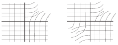
Figure 21: Other behavior.

5.2 Examples.

The following two examples show that the classes determined in Theorem 5.1.1 are non-empty.

5.2.1 Example 1.

We will show an example that admits stable and unstable curves that do not intersect each other and verifies the conditions shown in Theorem 5.1.1.

Construction. Let us consider $f:I\kern-3.69995ptR^{2}\rightarrow I\kern-3.69995ptR^{2}$ defined by

$$f(x,y)=\left(\begin{array}[]{cc}2&0\\ 0&1/2\\ \end{array}\right)\left(\begin{array}[]{c}x\\ y\\ \end{array}\right).$$

Consider the restriction of $f$ to the region

$$\Omega=\{(x,y):x\geq 0,\ y\geq 0,\ xy<1\}.$$

We will construct an extension to the whole quadrant of the linear automorphism restricted to the region $\Omega$. Each point $(k,1/k)$ on the hyperbola $xy=1$ determines a stable segment parameterized by $(k,u)$, with $0\leq u\leq 1/k$ and an unstable segment parameterized by $(v,1/k)$, with $0\leq v\leq k$. Such segments will correspond to semi straight lines defined by: the semi straight line corresponding to the stable segment parameterized by $(k,u)$, with $0\leq u\leq 1/k$, defined by $y=1/k(x-k)$ and the semi straight line corresponding to the unstable segment parameterized by $(v,1/k)$, with $0\leq v\leq k$, defined by $y=1/k(1+x)$. Let $H:\Omega\rightarrow I\kern-3.69995ptR^{2}$ be such that

$$H(x_{0},y_{0})=\left(\frac{x_{0}(1+y_{0})}{1-x_{0}y_{0}},\frac{y_{0}(1+x_{0})}{1-x_{0}y_{0}}\right),$$

$H(x_{0},0)=(x_{0},0)$ and $H(0,y_{0})=(0,y_{0})$ (see figure 22).

\psfrag{x0}{$x_{0}$}\psfrag{1x0}{$1/x_{0}$}\psfrag{y0}{$y_{0}$}\psfrag{1y0}{$1/y_{0}$}\psfrag{Hx0y0}{$H(x_{0},y_{0})$}\includegraphics[scale={0.25}]{fig300.eps}

Figure 22: Construction

Let $\Lambda$ be the first quadrant determined by the stable and unstable curves of the fixed point. We define $F:\Lambda\rightarrow\Lambda$ such that $F=HfH^{-1}$. Since $F$ is conjugated to a restriction of the linear automorphism we can define, for $F$, the Lyapunov function $L(p_{1},p_{2})=D(H^{-1}(p_{1}),H^{-1}(p_{2}))$, where $D=D_{s}+D_{u}$ is the metric Lyapunov function associated to $f$. The example we built verifies condition HL and hypothesis HA since it is conjugated to a restriction of the linear automorphism (see Theorem 5.1.1).

Remark 5.2.1

The images of the stable and unstable segments of $f$ under $H$ are $L$-stable curves and $L$-unstable curves of $F$. However a simple calculation shows that this semi-straight lines are not stable and unstable curves in the sense of the usual metric on the plane. The following example, will verify that its $L$-stable curve and $L$-unstable curve are also stable and unstable curves in the sense of the usual metric.

5.2.2 Example 2.

Construction. Let us consider $f:I\kern-3.69995ptR^{2}\rightarrow I\kern-3.69995ptR^{2}$ defined by

$$f(x,y)=\left(\begin{array}[]{cc}2&0\\ 0&1/2\\ \end{array}\right)\left(\begin{array}[]{c}x\\ y\\ \end{array}\right).$$

Let us consider the restriction of $f$ to region

$$\Omega=\{(x,y):x\geq 0,\ y\geq 0,\ xy<1\}.$$

We will construct an extension to the whole quadrant of the linear automorphism restricted to the region $\Omega$. Each point $(k,1/k)$ on the hyperbola $xy=1$ determines a stable segment parameterized by $(k,u)$, with $0\leq u\leq 1/k$ and an unstable segment parameterized by $(v,1/k)$, with $0\leq v\leq k$. Such segments will correspond to polygonal lines that will be constructed the following way:

• Case $k\leq 1/2$. The polygonal line corresponding to the stable segment parameterized by $(k,u)$, with $0\leq u\leq 1/k$ is defined by: $(k,u)$, when $0\leq u\leq 1/k-1$ and is then followed by a semi-straight line with slope $1/k$. The polygonal line corresponding to the unstable segment parameterized by $(v,1/k)$, with $0\leq v\leq k$ is defined by: $(v,1/k)$, when $0\leq v\leq k-\frac{k}{1+1/k}$, and is then followed by a semi-straight line with slope $1/k$ (see figure 23).

• Case $k\geq 2$. For this case we would use similar arguments to those used in the previous case.

  \psfrag{k0}{$k_{0}$}\psfrag{1/2}{$1/2$}\psfrag{2}{$2$}\psfrag{k}{$k$}\psfrag{y=1/k}{$y=1/k$}\psfrag{1}{$1$}\includegraphics[scale={0.3}]{fig51.eps}

  Figure 23: Construction

• Case $1/2\leq k\leq 2$. Note that the coordinates of the point where the polygonal line corresponding to the stable segment parameterized by $(1/2,u)$, with $0\leq u\leq 2$, breaks is $(1/2,2-1)$ and it is point $(2,1/2-1/6)$ for the case corresponding to the stable segment $(2,v)$ with $0\leq v\leq 1/2$. Let $f:[1/2,2]\rightarrow I\kern-3.69995ptR$ be the linear function such that $f(1/2)=1$ y $f(2)=1/6$. The polygonal line corresponding to the stable segment parameterized by $(k,u)$ is defined by: $(k,u)$, when $0\leq u\leq 1/k-f(k)$, and is then followed by a semi-straight line with slope $1/k$. Let $k_{0}<k$ be such that the length of the vertical segment included in the line $x=k_{0}$ between $y=1/k$ and the hyperbola $xy=1$ is $f(k_{0})$. The polygonal line corresponding to the unstable segment parameterized by $(v,1/k)$, with $0\leq v\leq k$ is defined by: $(v,1/k)$ for $0\leq u\leq k_{0}$, and is then followed by a semi straight-line with slope $1/k$ (see figure 23).

This way, we can define a homeomorphism $H$ that takes the invariant region $\Omega$ in the first quadrant $\Lambda$, sending the intersection of a stable segment with an unstable segment into the intersection of the corresponding polygonal. Let $F:\Lambda\rightarrow\Lambda$ be such that $F=HfH^{-1}$. Since $F$ is conjugated to a restriction of the linear $f$, we can define a Lyapunov metric function for $F$, $L(p_{1},p_{2})=D(H^{-1}(p_{1}),H^{-1}(p_{2}))$, where $D=D_{s}+D_{u}$ is the Lyapunov function associated to $f$. The constructed example verifies condition HL and hypothesis HA since it is conjugated to a restriction of a linear automorphism (preserving stable and unstable curves) (see Theorem 5.1.1).

Remark 5.2.2

Polygonal lines constructed in this example are stable (unstable) curves of $F$ not only on a Lyapunov function $L$ sense, but also in the usual metric sense.

Proof: Let us take as an example two points $p,q$ that are in the same unstable polygonal line, see figure 24. Because of the construction built before, the length of the unstable segment $AB$ tends to zero for the past with the same order that $\frac{1}{y^{2}}$ when $y$ tends to infinity. While the length of segment $H^{-1}(p),H^{-1}(q)$ does it with order $1/y$.

\psfrag{A}{$A$}\psfrag{B}{$B$}\psfrag{H-1p}{$H^{-1}(p)$}\psfrag{H-1q}{$H^{-1}(q)$}\psfrag{p}{$p$}\psfrag{q}{$q$}\psfrag{1}{$1$}\includegraphics[scale={0.25}]{fig53.eps}

Figure 24: Stable and unstable

Then, iterating for the past, points $f^{-n}(H^{-1}(p)),f^{-n}(H^{-1}(q))$ get inside the zone where $H$ is the identity and therefore the usual distance between $F^{-n}(p),F^{-n}(q)$ tends to zero when $n$ tends to infinity. $\Box$

References

[1]L. Brouwer,
Beweis des ebenen Translationssatzes,
Math. Ann. 72(1912), 37–54
[2]A. Fathi; F. Laudenbach; V. Poenaru,
Travaux de Thurston sur les surfaces (Seminaire Orsay),
Asterisque, (1979), 66–67
[3]J. Franks,
A new proof of the Brouwer plane translation theorem,
Ergod. Th. and Dynamic. Sys., 12(1991), 217–226
[4]J. Groisman,