Signatures of Alfvén waves in the polar coronal holes as seen by EIS/Hinode

Abstract

Context. We diagnose the properties of the plume and interplume regions in a polar coronal hole and the role of waves in the acceleration of the solar wind.

Aims. We attempt to detect whether Alfvén waves are present in the polar coronal holes through variations in EUV line widths.

Methods. Using spectral observations performed over a polar coronal hole region with the EIS spectrometer on Hinode, we study the variation in the line width and electron density as a function of height. We use the density sensitive line pairs of Fe xii 186.88 Å & 195.119 Å and Fe xiii 203.82 Å & 202.04 Å .

Results. For the polar region, the line width data show that the nonthermal line-of-sight velocity increases from $26\ {\rm km\;s}^{-1}$ at 10^′′ above the limb to $42\;{\rm km\;s}^{-1}$ some 150^′′ (i.e. $\sim$110,000 km) above the limb. The electron density shows a decrease from $3.3\times 10^{9}\ {\rm cm}^{-3}$ to $1.9\times 10^{8}\ {\rm cm}^{-3}$ over the same distance.

Conclusions. These results imply that the nonthermal velocity is inversely proportional to the quadratic root of the electron density, in excellent agreement with what is predicted for undamped radially propagating linear Alfvén waves. Our data provide signatures of Alfvén waves in the polar coronal hole regions, which could be important for the acceleration of the solar wind.

1 Introduction

Over the past decade, data from Ulysses show the importance of the polar coronal holes, particularly at times near solar minimum, for the acceleration of the fast solar wind. Acceleration of the quasi-steady, high-speed solar wind requires additional energy in the supersonic region of the flow. It has been shown theoretically that Alfvén waves from the Sun can accelerate the solar wind to these high speeds. Until now this is the only mechanism shown to enhance the flow speed of the basically thermally driven wind to the high flow speeds observed in interplanetary space. The Alfvén speed in the corona is quite high, so Alfvén waves can carry a significant energy flux even for low wave energy density. Direct observations of Alfvén waves has gained momentum after the launch of the Hinode satellite. Recent reports of detections of low-frequency ($<$ 5 mHz), propagating Alfvénic motions in the solar corona (Tomczyk et al., 2007, from coronagraphic observations) and chromosphere (De Pontieu et al., 2007b) and their relationship with chromospheric spicules observed at the solar limb (De Pontieu et al., 2007a) with the Solar Optical Telescope (SOT; Tsuneta et al., 2008b) on Hinode (Kosugi et al., 2007) have widened interest in the subject. If MHD waves play an important role in accelerating high-speed streams and coronal heating, then this should be observed via a broadening of spectral lines, increasing with radial distance in the inner corona.

There have been several off-limb spectral line observations to search for Alfvén wave signatures. Measurements of ultraviolet Mg x line widths during a rocket flight showed an increase in width with height to a distance of 70,000 km (Hassler et al., 1990). Also, coronal hole Fe x spectra taken at Sacramento Peak Observatory showed an increase in the line width with height (Hassler & Moran, 1994). SUMER/SoHO (Wilhelm et al., 1995) were used to record the off-limb, height-resolved spectra of an Si viii density sensitive line pair, in equatorial coronal regions (Doyle et al., 1998; Wilhelm et al., 2005) and in polar coronal holes (Banerjee et al., 1998; Wilhelm et al., 2004). The measured variation in line width with density and height supports undamped wave propagation in coronal structures. This was strong evidence of outwardly propagating undamped Alfvén waves in the corona, which may contribute to coronal heating and high-speed solar wind in the case of coronal holes. We revisit the subject with the new EIS instrument on Hinode and compare with our previous results as recorded by SUMER/SoHO. In the present study, we also make a full scan in the off-limb polar region to study the differences between the plume and interplume regions and to address the question as to whether the plume or the interplume is the preferred channel for the acceleration of the wind. Analyses of SUMER (e.g. Banerjee et al., 2000; Teriaca et al., 2003) and UVCS (e.g. Giordano et al., 2000) data have shown that the width of UV lines in interplumes is greater than in plume regions, indicating that interplumes as the site where energy is preferentially deposited and, possibly, the fast wind emanates. In this letter we concentrate on the density diagnostic capability of the density-sensitive line pairs of Fe xii 186.88 Å and 195.119 Å (Young et al., 2009) and Fe xiii 203.82 Å and 202.04 Å (Watanabe et al., 2009) for the off-limb coronal hole region. From a study of the variation of line width of the strongest line within our spectrum, we try to find signatures of propagating Alfvén waves.

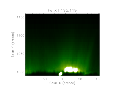
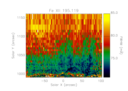
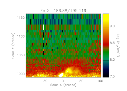
Figure 1: Images of the north polar coronal hole off-limb region. From top to bottom: intensity, width, and density obtained from Fe xii lines.

2 Observation and data reduction

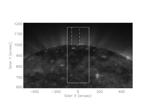
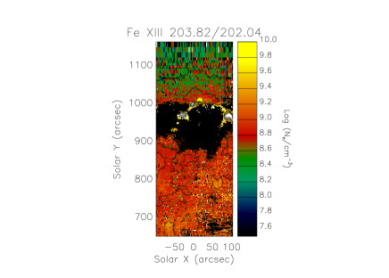
Figure 6: The left panel shows the EIT 171 Å image with EIS field of view overplotted (square box) and plume and interplume chosen. The right panel shows the density map corresponding to the full EIS raster scan as recorded by Fe xiii and the contours show the intensity.

EIS onboard Hinode observes high-resolution spectra in two wavelength bands 170-211 Å and 246-292 Å with a spectral resolution of 0.0223 Å per pixel (Culhane et al., 2007). We observed the north polar coronal hole on and off the limb with the 2^′′ slit on 10 October 2007 (see left panel of Fig. 6, available online only, for a context image). The raster was run for more than four hours with 101 exposures of 155 s, covering an area of 201.7^′′$\times$512^′′. We used the study arm_raster_ar, which was designed with nine windows containing lines from Fe viii, Fe x, Fe xi, Fe xii, Fe xiii, Fe xiv, Fe xv, He ii, Mg vi, O v, O vi, Si vii, and Al ix. All data have been reduced and calibrated with the standard procedures as given in the SolarSoft(SSW) library. These standard subroutines include dark current subtraction, cosmic ray removal, flat field, hot pixel correction, and absolute calibration. We use the density sensitive line pairs of Fe xii 186.88 Å and 195.119 Å (Young et al., 2009) and Fe xiii 203.82 Å and 202.04 Å (Watanabe et al., 2009) for density diagnostics and use the strongest line of Fe xii 195.119 Å for the line width study. These lines are formed in the temperature range of $T$ = 1 to 2 MK. One can see from the CHIANTI (Landi et al., 2006) atomic data base that these line pairs have a very good density sensitivity between 7.0 $\leq$ $\log$ N_e (cm^-3) $\leq$ 10.0.

The Fe xii 195.12 Å was fitted using a double Gaussian (see Young et al., 2009), considering the two main transitions at 195.119 and 195.179 Å (with a 5% contribution on average to the stronger component). The two transitions for Fe xii at 186.854 and 186.887 were fitted with a single Gaussian at 186.88 Å. For Fe xiii, the new CHIANTI updated version was used, which incorporates new Fe ion models as described in Watanabe et al. (2009). To address the issue of weaker signal-to-noise as we go off-limb, a variable binning in the radial direction was performed, where after 1010^′′ we initially binned over 27 pixels, finishing by binning over 42 pixels far off-limb. For Fe xiii we also binned over 5 spectra in the X direction. The “grating tilt” reported by Young et al. (2009), which clearly affects line ratios, was corrected by assuming that the tilt is linear and using the value found by Young et al. (2009) after our own comparison.

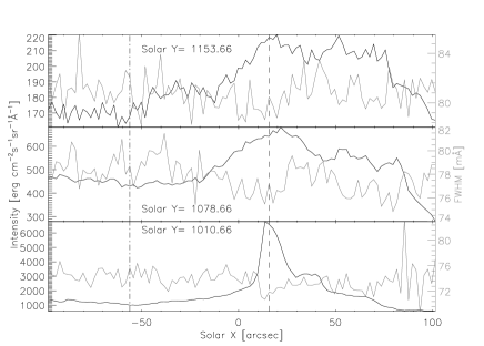
Figure 2: A plot of the intensity (solid lines) and FWHM (grey lines) as recorded by Fe xii 195 Å along three strips tangent to the limb at different heights to illustrate the anti-correlation between intensity and velocity. The vertical lines show the position of the plume (dashed) and interplume (dot-dashed). The limb corresponds to Y=1003, as decided from the intensity peak of a low temperature line, Si vii.

3 Results

The spectral line profile of an optically thin coronal emission line results from the thermal broadening caused by the ion temperature $T_{i}$, as well as by small-scale unresolved nonthermal motions and/or unresolved flows. Assuming that the instrumental profile can be expressed as Gaussian, the expression for the full width half maximum (FWHM) is given as

$$FWHM\,=\,\left[W^{2}_{inst}+4ln2\,\left(\frac{\lambda}{c}\right)^{2}\,\left(\frac{2\,k\,T_{i}}{M_{i}}\,+\,{\xi}^{2}\right)\right]^{1/2}$$ (1)

where $T_{i}$, $M_{i}$, and $\xi$ are respectively the ion temperature, ion mass, and nonthermal velocity, while $W_{inst}$ is the instrumental width (for the 2^′′ slit we use 62 mÅ ), with the ion temperature assumed equal to the peak in the line formation temperature as given by CHIANTI.

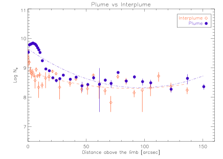
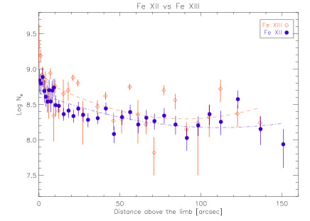
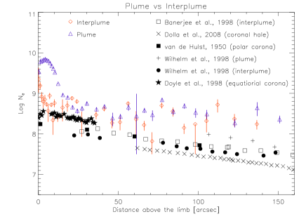
Figure 3: Variation in density with height in the polar coronal hole region. The top panel shows results as recorded by Fe xiii, along plume and interplume regions. The middle panel shows the comparison of Fe xii and Fe xiii. The lower panel shows a comparison of density values as recoded by different instruments within the same radial distance.

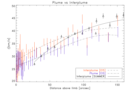
Figure 4: Variation in nonthermal velocity with height as recorded by Fe xii 195 Å along a polar plume and interplume (the present study). The solid line corresponds to the nonthermal velocity as derived from Si viii 1445.75Å (Banerjee et al., 1998). The dashed line is a third-order polynomial fit.

Fig. 1 shows maps of line intensity and FWHM from Fe xii 195.12 Å and electron density (from Fe xii) of the northern polar off-limb coronal hole region.

Observations have revealed that plasma conditions in polar plumes are quite different from interplume lanes (Hassler et al., 1997; Wilhelm et al., 1998). From these maps it is clear that plumes have slightly higher density and lower FWHM. Closer to the limb at the base of the plume (around $X=15$) one also finds the presence of a coronal bright point and it does affect the density values close to the limb. To look for a possible correlation/anti-correlation between the line intensity and the most probable speed, we concentrate on specific heights. As we go off the limb, Fig. 2 shows the line intensity and the FWHM along three strips tangent to the limb at different heights. We find evidence of an anti-correlation between the intensity and FWHM. If we go out farther away from the limb, the anti-correlation is weaker, because at these heights above the limb the plume structures have expanded slightly nonradially (see Fig. 1). This observed anti-correlation between intensity and width in polar plumes have been reported by Antonucci et al. (1997) and Noci et al. (1997) with the UVCS instrument and also by Hassler et al. (1997) and Banerjee et al. (2000) with SUMER. Now, to study the variations of different parameters namely density and FWHM with height, we focus our attention on a fixed location, $X=15$, as a representative location for the plume and $X=-57$, as a representative case for the interplume.

In Fig. 3 we plot the variation of the density with height as recorded by Fe xiii (top panel) along plume and interplume (along the two dashed vertical lines as drawn in Fig. 2). The dashed lines in Fig. 3 correspond to a second order polynomial fit. One can clearly see that at the solar limb, the plume density is almost one order of magnitude higher than the interplume, but around 70^′′  off-limb, the densities of the plume and interplume seem to be very close. The errors in deriving the electron density in Fig. 3 depends not only on the line strengths but also on the uncertainty within the atomic data, which can be upto 20% (Del Zanna & Mason, 2005). We should point out here that, for polar regions, these densities are higher than the previously published values. To validate our measurements, we also calculated the densities using Fe xii lines. For the same range of heights and along the same interplume lane, we compare the results in the middle panel of Fig. 3. It clearly shows that the densities are consistent (within their error bars) as recorded by two different line pairs of Fe xiii and Fe xii. In the lower panel of Fig. 3 we show a detailed comparison of our measured densities with earlier published values for the same range of heights for different coronal conditions (Wilhelm et al., 1998; van de Hulst, 1950; Dolla & Solomon, 2008).

Our densities are marginally comparable to previously published values for plumes and for the quiet corona. This may stem form the new atomic data for Fe xiii and Fe xiii used in this analysis and/or contamination from the background quite sun. Assuming ionisation equilibrium and using Eq. (1), we now calculate the nonthermal speed and study its variation with height (see Fig. 4) for the Fe xii (as this is the strongest line and line widths are measured with better accuracies). The variation in the nonthermal velocity with height along the plume and interplume reveals that, consistently with height, the nonthermal velocity is slightly higher in the interplume than the plume. For comparison with previously reported results, we overplot the nonthermal velocity as derived from Si viii 1445.75Å (Banerjee et al., 1998) as represented by triangles along with their best fit in Fig. 4.

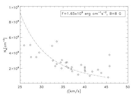
Figure 5: Variation in electron density with nonthermal velocity for the polar coronal hole. The squared boxes represents the observed values and the solid line represents the theoretical relation (Eq. [4]) for fixed magnetic field strength as indicated.

4 Discussion and conclusions

Using the EIS spectrometer on Hinode, we have studied the variations in the line width and the electron density as a function of height. We used the density sensitive line pairs of Fe xii and Fe xiii, and calculated densities have comparable values (within their error bars). We must point out that the densities as reported here are consistently higher than previously published values (see Fig. 3). The difference may stem from real physical differences between the emitting regions of the coronal hole plasma around November 2007 and previous coronal conditions as recorded by other instruments (e.g. SUMER). Other factors could be the CHIANTI atomic models. There has been a recent revision in the Fe xiii atomic model (Watanabe et al., 2009), and we used the updated CHIANTI database for our calculation. We should also point out that, from the full scan image of the density (Fig. 6, available in the online version only), it shows that the off-limb coronal densities are close to the quiet Sun values and in fact somewhat higher than the on-disk coronal hole densities. This suggests that the coronal emission may have been affected by background emission from the quiet coronal structures.

Alfvén waves propagate virtually undamped through the quasi-static corona and deposit their energy flux in the higher corona. The total energy flux crossing a surface of area $A$ in the corona due to Alfvén waves is given by (Moran, 2001)

$$F=\sqrt{\frac{\rho}{4\pi}}<\delta v^{2}>B\ A\leavevmode\nobreak\ \leavevmode\nobreak\ ,$$ (2)

where $\rho$ is the plasma mass density (related to $N_{e}$ as $\rho=m_{p}N_{e}$, $m_{p}$ is the proton-mass), $<\delta v^{2}>$ is the mean square velocity related to the observed nonthermal velocity as $\xi^{2}=<\delta v^{2}>/2$, and $B$, is the magnetic field strength. If the wave energy flux is conserved as the wave propagate outwards, then Eq.(2) gives

$$<\delta v^{2}>^{1/2}\ \propto\ \rho^{-1/4}(BA)^{-1/2}\leavevmode\nobreak\ \leavevmode\nobreak\ ,$$ (3)

Now if one assumes a flux tube geometry, then $BA$ is constant with height and Eq.(3) yields

$$<\delta v^{2}>^{1/2}\ \propto\ \rho^{-1/4}\leavevmode\nobreak\ \leavevmode\nobreak\ .$$ (4)

From our dataset (for Fe xii 195 Å ) at 30^′′ above the limb for the interplume location (see Table. LABEL:table) using $N_{e}=2.2\times 10^{8}\leavevmode\nobreak\ {\rm cm}^{-3}$, $<\delta v^{2}>=2\times(43.7\leavevmode\nobreak\ {\rm km\leavevmode\nobreak\ s}^{-1})^{2}$, we find $F=1.85\times 10^{6}$ ergs cm^-2 s^-1 for $B=8$ G, which is only slightly higher than the requirements for a coronal hole with a high-speed solar wind flow (Withbroe & Noyes, 1977), which is in turn estimated to be $8\times 10^{5}$ ergs cm^-2 s^-1. The average field strength in coronal holes is estimated to be 5-10 G (Hollweg, 1990; Tsuneta et al., 2008a).

To explore the validity of Eq.(4), we plot Fig. 5 corresponding to our interplume data. The solid lines are the theoretically predicted functional form of the variation of number density with nonthermal velocity (Eq.[4]) and the diamonds are our observed data. The proportionality constant have been chosen to match the calculated energy flux. For the interplume data we used B=8 G. Once again the agreement is very good, especially when we are away from the limb.

Our observations provide observational signatures for the presence of Alfvén waves in polar coronal regions at least within 1.1$R_{\odot}$. These upwardly propagating Alfvén waves may heat the corona and accelerate the solar wind. The slightly larger widths within the interplume regions as compared to plumes also indicate that probably interplumes are the preferred channel for the acceleration of the wind. In this dataset we do not find large differences between plumes and interplumes beyond 70^′′above the limb. Finally the EIS line width results are consistent with previous results from SUMER.

1

Table 1: A summary of measured intensity, calculated nonthermal velocity ($\xi$), flux ratio and electron density for the plume (P) and interplume (I-P) obtained from Fe xii ($T_{i}=1.3\times 10^{6}$K) and Fe xiii ($T_{i}=1.6\times 10^{6}$K) at different locations.

Above limb	I(195.12Å)		$\xi$		Fe xii ratio		$\log N_{e}/cm^{-3}$		I(202.04Å)		$\xi$		Fe xiii ratio		$\log N_{e}/cm^{-3}$
(arcsec)	erg cm2s-1sr-1		km s-1		$10^{-2}$				erg cm2s-1sr-1		km s-1		$10^{-2}$
	I-P	P	I-P	P	I-P	P	I-P	P	I-P	P	I-P	P	I-P	P	I-P	P
0.00	52.45	164.67	34.6	36.9	20.25	22.71	8.84	8.95	34.35	93.85	20.7	24.9	50.52	64.70	9.35	9.53
1.00	62.02	235.34	29.3	38.4	19.27	24.54	8.80	9.03	41.81	137.62	26.1	27.9	38.72	84.76	9.19	9.78
2.00	69.19	338.49	28.3	39.6	21.29	25.57	8.89	9.07	48.19	190.09	22.2	27.6	22.87	86.29	8.92	9.80
3.00	75.52	466.16	29.7	35.1	17.08	26.58	8.69	9.11	52.97	249.19	29.2	28.1	17.85	87.73	8.80	9.82
4.00	78.00	591.03	26.7	33.5	15.42	27.77	8.61	9.15	57.13	304.34	25.9	28.0	19.98	88.91	8.85	9.84
5.00	77.34	675.66	24.7	29.2	14.12	29.85	8.54	9.23	60.63	341.56	31.7	28.8	15.58	87.72	8.73	9.82
6.00	77.36	723.83	24.5	27.3	17.29	31.22	8.70	9.28	64.50	361.62	35.6	28.6	10.73	86.09	8.57	9.80
7.00	79.45	706.95	26.0	25.5	14.13	32.34	8.54	9.32	65.34	363.00	29.4	25.5	23.97	82.00	8.94	9.75
8.00	79.13	664.77	23.0	25.2	17.20	32.43	8.70	9.32	65.01	347.64	29.3	24.1	15.04	77.39	8.72	9.68
9.00	81.20	592.35	30.8	25.1	18.07	31.95	8.74	9.31	66.42	318.12	28.2	24.1	6.45	71.80	8.34	9.61
10.00	80.88	505.33	32.0	24.1	13.21	31.79	8.49	9.30	67.35	277.62	29.7	25.3	16.50	63.80	8.76	9.52
12.00	80.63	339.73	29.9	22.1	13.02	29.52	8.48	9.22	66.44	183.97	29.8	25.9	7.67	42.09	8.41	9.24
15.00	78.40	201.39	30.5	28.4	11.05	19.71	8.36	8.82	65.57	125.56	33.0	28.2	12.94	25.23	8.65	8.96
18.00	73.91	165.77	30.8	30.4	11.85	15.40	8.41	8.61	67.02	113.20	30.8	26.6	14.58	22.32	8.70	8.90
21.00	71.94	144.86	34.3	29.4	10.61	12.68	8.34	8.46	61.95	103.00	31.1	27.9	21.06	13.27	8.88	8.66
24.00	68.51	131.47	33.0	27.3	12.33	13.57	8.44	8.51	60.72	97.82	31.6	28.2	18.04	10.72	8.80	8.57
27.00	66.44	121.21	33.1	28.4	10.90	11.48	8.35	8.39	59.08	95.80	33.7	30.7	6.55	12.26	8.34	8.63
30.00	63.69	116.30	34.2	27.0	9.80	10.66	8.28	8.34	56.08	89.60	31.6	31.2	0.70	16.14	7.50	8.75
36.00	57.09	100.84	31.9	29.7	10.15	11.06	8.31	8.36	52.96	81.91	32.2	29.4	8.66	11.76	8.47	8.61
41.00	53.43	93.63	31.7	27.3	12.38	9.21	8.44	8.24	50.69	76.62	35.4	30.1	12.21	13.79	8.62	8.68
46.00	52.43	86.73	35.8	28.1	7.16	9.12	8.08	8.24	48.36	71.34	35.6	32.9	5.60	7.19	8.27	8.39
51.00	48.57	81.15	33.5	33.0	10.38	10.60	8.32	8.34	46.97	70.03	35.1	32.0	5.76	8.00	8.29	8.43
56.00	46.51	74.57	36.5	32.6	11.52	9.66	8.39	8.27	43.59	61.55	35.0	31.9	16.10	13.13	8.75	8.66
61.00	42.88	65.98	34.4	31.4	8.86	11.49	8.22	8.39	40.57	57.00	36.3	31.5	6.72	8.19	8.36	8.44
66.00	39.34	61.77	37.4	32.6	10.24	10.56	8.31	8.33	39.13	52.93	34.3	32.6	4.94	11.07	8.22	8.58
71.00	40.04	57.45	40.4	33.3	9.55	8.65	8.27	8.20	36.33	50.11	35.7	32.6	2.08	8.64	7.82	8.47
77.00	36.04	52.79	37.4	34.8	10.70	9.90	8.34	8.29	34.49	46.50	39.7	35.4	14.54	19.55	8.70	8.84
84.00	31.71	46.21	37.4	32.6	8.86	9.20	8.22	8.24	29.95	41.55	40.9	35.8	10.53	10.27	8.56	8.55
91.00	29.47	41.63	38.5	35.8	6.55	6.95	8.03	8.06	26.83	36.19	38.6	35.8	4.22	14.17	8.15	8.69
98.00	26.06	36.87	39.1	35.6	8.68	9.05	8.20	8.23	24.20	32.70	44.6	40.2	5.23	9.89	8.24	8.53
105.00	24.47	34.22	43.1	34.1	11.04	10.78	8.36	8.35	22.11	29.07	35.3	32.3	6.19	9.02	8.32	8.49
112.00	23.00	31.14	37.4	34.6	9.39	6.49	8.25	8.02	21.09	29.55	41.2	38.9	14.96	-2.76	8.72	****
122.50	20.49	28.04	43.0	39.0	14.76	9.86	8.57	8.29	17.72	24.00	40.2	37.4	6.88	5.61	8.37	8.27
136.50	16.80	22.50	41.1	39.8	8.02	5.26	8.15	7.89	14.61	19.07	37.5	37.4	5.24	12.69	8.24	8.64
150.50	14.68	18.72	42.7	40.3	5.66	8.82	7.94	8.21	12.31	15.80	44.0	39.5	0.05	6.85	7.50	8.36

7