A Random Force is a Force, of Course, of Coarse:
Decomposing Complex Enzyme Kinetics with Surrogate Models

Abstract

The temporal autocorrelation (AC) function associated with monitoring order parameters characterizing conformational fluctuations of an enzyme is analyzed using a collection of surrogate models. The surrogates considered are phenomenological stochastic differential equation (SDE) models. It is demonstrated how an ensemble of such surrogate models, each surrogate being calibrated from a single trajectory, indirectly contains information about unresolved conformational degrees of freedom. This ensemble can be used to construct complex temporal ACs associated with a “non-Markovian” process. The ensemble of surrogates approach allows researchers to consider models more flexible than a mixture of exponentials to describe relaxation times and at the same time gain physical information about the system. The relevance of this type of analysis to matching single-molecule experiments to computer simulations and how more complex stochastic processes can emerge from a mixture of simpler processes is also discussed. The ideas are illustrated on a toy SDE model and on molecular dynamics simulations of the enzyme dihydrofolate reductase.

I Introduction

When enzymes and other proteins are probed at the single-molecule level, it has been observed in both experiments xie_dynamicdis_98 ; xie04 ; Dobson_science06AdK ; natureFRET07 and simulation studies wolynes_crackingPNAS03 ; AdK ; wolynesHFSP08 ; arora09 ; rief_09 ; Portman_CaMcracking09 that conformational fluctuations at several disparate timescales have physically significant influence on both large scale structure and biochemical function. In this article, a method for using a collection of Marovian surrogate models SPA1 ; SPA2 ; SPAJCTC to predict kinetics that would often be considered non-Markovian is presented klafter08 ; kou_08 . The ideas in SPAJCTC are extended to treat a system with more complex kinetics. The aim of the approach is to obtain a better quantitative understanding the factors contributing to complex time autocorrelations (ACs) associated with quantities modulated by slowly evolving conformational degrees of freedom. The focus is on systems where certain thermodynamically important conformational degrees of freedom evolve over an effective free energy surface with relatively low-barriers; this situation is often relevant to molecules undergoing a “population shift” or “selected-fit” mechanism AdK ; arora09 and the connection to “dynamic disorder” xie_dynamicdis_98 is also discussed. The particular enzyme studied is dihydrofolate reductase (DHFR) because of its biological relevance to therapeutics and also due to the rich kinetics observed in certain order parameters arora09 .

Surrogate models are used to describe the short time dynamics. These surrogates are fairly simple phenomenological parametric stochastic differential equation (SDE) models. Specifically the Ornstein-Ulhlenbeck process and an overdamped Langevin equation with a position dependent diffusion function hummer_posdep ; SPA1 ; wangPNAS07 ; SPAJCTC are considered as the candidate surrogate models. Position dependent diffusion is often observed when a few observables (or order parameters) are used to describe an underlying complex system such as a protein. Position dependent noise models allow one to consider ACs having a different functional form than an exponential decay and it is demonstrated that this added flexibility can be of assistance in both understanding short and long timescale kinetics. Maximum likelihood type estimates utilizing transition densities, exact and approximate aitECO ; ozaki ; chen09 , are used to fit our surrogate SDE models. The fitting method does not require one to discretize hummer_posdep state space (the surrogates assume a continuum of states). The temporal AC is not used directly as a fitting criterion kou_08 ; stuart_09 , but the surrogate models are able to accurately predict the AC after the model parameters are fit. Maximum likelihood based approaches employing accurate transition density approximations and a parametric structure posses several advantages in this type of application llglassy . An accurate transition density of a parametric SDE facilitates goodness-of-fit tests appropriate for both stationary aitFAN05 ; chen08 and nonstationary time series hong . The latter is particularly relevant to many systems (like the one considered here) where the diffusion coefficient is modulated by factors not directly monitored klafter08 ; SPAJCTC and the hypothesis of a fixed/stationary surrogate model describing the modeled time series is questionable. Statistically testing the validity of various assumptions explicitly or implicitly behind a candidate surrogate model, such as Markovian dynamics, state dependent noise and/or regime switching is helpful in both experimental and simulation data settings SPAfilter ; SPAdsDNA .

The type of modeling approach presented is attractive from a physical standpoint for a variety of reasons. The items that follow are discussed further in the Results and Discussion:

• In situations where the magnitude of the local fluctuations depend significantly on the instantaneous value of the order parameter monitored, simple exponential (or a finite mixture of exponentials socci96 ) can be inadequate to describe the relaxation and/or AC function SPAJCTC . The surrogates proposed can account for this situation when overdamped diffusion models can be used; additionally the estimated model parameters can be physically interpreted.

• It has been observed that even in single-molecule trajectories that “dynamic disorder” can be observed due to ignoring certain conformational degrees of freedom xie_dynamicdis_98 ; xie04 ; klafter08 ; the methods proposed here can be used to account for this type of variability and show promise for comparing frequently sampled single-molecule experimental time series to computer simulations where dynamic disorder is relevant.

• Changes in conformational fluctuation magnitudes have been suggested to lead to physically interesting phenomena, so possessing a means for quantitatively describing an ensemble of dynamical responses can help one in better understanding the complex dynamics of enzymes, e.g. wolynes_crackingPNAS03 ; AdK ; wolynesHFSP08 ; Portman_CaMcracking09 .

• There is general interest in showing how more complex stochastic processes arise from a collection of simpler parts granger80a ; granger80b ; cox91 ; klafter09 . We discuss how, within a single trajectory, a continuous type of regime switching of Markovian surrogate models gives rise to an AC that would be considered non-Markovian.

The remainder of this article is organized as follows: Section II reviews the background and presents the models considered. Section III introduces the new modeling procedure used to approximate the AC function of a molecule experiencing multiple types of fluctuations. Section IV presents the Results and Discussion, Section V provides the Summary and Conclusions and this is followed by an Appendix.

II Background and Methods

II.1 Effective Dynamics and Statistical Inference

The trajectory generated by a detailed molecular dynamics (MD) simulation will be denoted by $\{z_{i}\}_{i=1}^{N}$. The dynamics of the order parameter monitored is assumed to be complex (nonlinear, modulated by unobserved factors, etc.) even at the relatively short $O(ns)$ time intervals the order parameter time series is observed over. However, over short $\approx 50-100ps$ time intervals a continuous stochastic differential equation (SDE) having the form

$$dz_{t}= \mu(z_{t};\theta,\Gamma)dt+\sqrt{2}\sigma(z_{t};\theta,\Gamma)dB_{t},$$ (1)

can often approximate the effective stochastic dynamics of the order parameter SPA1 ; SPAJCTC . In the above $\mu(\cdot)$ and $\sigma^{2}(\cdot)$ are the nonlinear deterministic drift and diffusion functions (respectively) and $B_{t}$ represents the standard Brownian motion raoDIFF . The finite dimensional parameter vector is denoted by $\theta$ and $\Gamma$ is used to represent unresolved lurking degrees of freedom that slowly modulate the dynamics gAIoan .

The surrogate SDE models are formed by first dividing each trajectory into $L$ temporal partitions. Each estimated parameter vector is denoted by $\theta_{\ell}$ using the sequence $\{z_{i}\}_{i=T_{\ell-1}}^{T_{\ell}}$ and an assumed model , where $\ell$ is an index of a partition, $1=:T_{0}<\ldots<T_{\ell}<\ldots<T_{L}:=N$, used to divide a time series into $L$ disjoint local temporal windows. Within each of these windows, the data and the assumed model structure is used to compute $\theta_{\ell}$ using maximum likelihood type methods (exact chen09 and approximate aitECO depending on the model). The parametric structures considered are presented in the next section. It is to be stressed that we estimate a collection of models, $\{\theta_{\ell}\}_{\ell=1}^{L}$ for each trajectory. The differences in the estimated parameters are due in part to random slowly evolving forces modulate the dynamics and also in part to unavoidable estimation uncertainty associated with a finite time series. It is demonstrated that a collection of surrogate model parameter vectors is needed to summarize conformational fluctuations inherent to many complex biomolecules. This procedure is repeated for each observed MD trajectory / time series.

The term “local diffusion coefficient” $\equiv\widetilde{D}(z;\Gamma):=\sigma^{2}(z;\theta,\Gamma)$ is introduced in order to distinguish the coefficient in the Eqn. 1 from the diffusion coefficient usually implied in the physical sciences: we estimate the former from observed data. The term “diffusion coefficient” used in statistical physics zwanzig is not necessarily the same as $\widetilde{D}(z;\Gamma)$. If $\Gamma$ does not modulate the dynamics, the two definitions are effectively identical. However one theme of this paper is that some traditional dynamical summaries of statistical physics, such as diffusion coefficient and ensemble based AC, can be modified or made less coarse by using a collection of surrogate models. Such a procedure may help in intpretting/understanding single-molecule time series.

II.2 Candidate Surrogate SDE Models

Two local parametric SDE models considered. MATLAB scripts illustrating how to obtain parameter estimates of both models from discretely observed data are available online www.caam.rice.edu/tech_reports/2008_abstracts.html#TR08-25. The first is a linear, constant additive noise process:

$$dz_{t}=B(A-z_{t})dt+\sqrt{2}CdB_{t}.$$ (2)

The above SDE has a rich history in both the physical sciences gardiner where it is usually referred to as the Ornstein-Uhlenbeck (OU) process and in econometrics where it is sometimes referred to as the Vasicek process chen09 . The parameter vector to estimate in this model is $\theta\equiv(A,B,C)$. This model is appealing for a variety of reasons, one being that the exact transition density and maximum likelihood parameter vector for a discretely sampled process can be written in closed-form, i.e. a numerical optimization is not needed to find the parameter vector because the parameter estimate can be written explicitly in terms of $\theta$ and the observed data chen09 .

The second is a nonlinear, position dependent overdamped (PDOD) Langevin type SDE schultenJCP04 ; SPA1 ; SPAJCTC :

$$dz_{t}= \beta\Big{(}C+D(z_{t}-\psi_{0})\Big{)}^{2}\Big{(}A+B(z_{t}-\psi_{0})\Big{)}dt$$ (3)

$$+\sqrt{2}\Big{(}C+D(z_{t}-\psi_{0})\Big{)}dB_{t}.$$

The variable $\beta\equiv 1/(k_{B}T)$ is the inverse of the product of Boltzmann’s constant and the system temperature. $\psi_{0}$ represents a free parameter; in this article it coincides with the umbrella sampling point specified in the simulation. The parameter vector to estimate in this model is $\theta\equiv(A,B,C,D)$. Each parameter is estimated using the observed data and the transition density expansions aitECO associated with Eqn. 3 is used to construct a log likelihood cost function. A Nelder-Mead search is then used to find the $\theta$ maximizing the associated cost function. The effective force in the above model is assumed to be linear in $z$, e.g. $F(z):=A+B(z-\psi_{0})$ whereas the diffusion function $\equiv\widetilde{D}(z;\Gamma):=\Big{(}C+D(z-\psi_{0})\Big{)}^{2}$ is quadratic in $z$. The overdamped appellation comes from multiplying the effective force by the effective friction (as determined by the Einstein relation schultenJCP04 ) corresponding to this diffusion function.

In this article, all stochastic integrals used are Itô integrals. When a complex high-dimensional system with multiple timescales is approximated with a low dimensional SDE possessing position dependent noise the choice of the Itô or Stratonovich integral influences the interpretation of the drift function and the issue of which interpretation is “physically correct” is a nontrivial problem razstuart04 ; dima . A related item is the so-called “noise-induced drift” risken ; arnold00 . Such a term is sometimes explicitly added to the drift arnold00 , one thermodynamic motivation for this is discussed further in Section VII.2.

An appealing feature of the data-driven modeling procedure presented here and elsewhere SPA1 ; molsim ; SPAfilter ; SPAJCTC ; gAIoan is that various SDE models, of an explicitly specified form, can be considered, estimated, and tested using observed trajectories. Statistical hypothesis tests making use of the conditional distribution (not just moments) of the assumed surrogate model can then be used to test if the model assumptions are justified for the observed data. Tools from mathematical statistics hong ; aitFAN05 facilitate quantitatively and rigorously testing if certain features are required to adequately describe the stochastic dynamics. Many features, e.g. position-dependent noise, would be hard to statistically check using AC based heuristic methods. Such heuristic checks are traditionally used in statistical physics, e.g. bussi_08 ; dima .

The data-driven models are used to approximate the stochastic evolution of black-box data and the estimated parameters do have a loose physical phenomenological interpretation. If one desires to compute unambiguous physical quantities from the estimated coefficients using a particular definition from statistical physics, the models can also be used to generate data for this purpose. For example, surrogate models can generate nonequilibrium (surrogate) work SPA1 ; SPA2 ; gAIoan and, under various assumptions, a well-defined thermodynamic potential of mean force (PMF) can be derived from such data hummerPNAS01 ; schultenJCP04 . This contrasts the case where one starts with a high dimensional stochastic process (of known functional form) and then uses stochastic analysis to reduce the dimensionality of the system by first appealing to asymptotic arguments razstuart04 and then possibly modifying the resulting equations to achieve a desired physical constraint arnold00 . In both analytical and data-driven cases, the goal is often to construct a single limiting low-dimensional evolution equation that can be used to predict statistical properties of the complex system valid over longer time-scales schultenJCP04 ; razstuart04 ; dima ; hummer_posdep . It is not quantitatively clear at what timescale such an approximation (if any such useful approximation exists at all) is valid over. Furthermore it is usually difficult to determine if an equilibrium concept such as a PMF connects simply to trajectory-wise kinetics in small complex systems experiencing fluctuations. Again, an appealing feature of the approach advocated here is that various statistical hypothesis tests hong ; aitFAN05 ; chen08 can be used to quantitatively assess the validity of proposed (reduced) evolution equations to see if physically convenient models are consistent with the observed data. For example, such tests can be used to determine the time one needs to wait before inertia can be neglected SPAJCTC .

Regarding the validity of using a single surrogate SDE to approximate “long term” $>O(ns)$ trends, a main underlying theme of this paper and others gAIoan ; SPA2 ; SPAJCTC ; SPAfilter is that the presence of a lurking slowly evolving degree of freedom, $\Gamma$, can significantly complicate using a single equation and that methods for quantitatively accounting for this sort of variation are underdeveloped. Information in these types of models have proven useful in both theoretical chemistry computations gAIoan ; SPA2 and in characterizing nanoscale experimental data SPAdsDNA ; SPAfilter ; SPAfric . Throughout this article, it is shown how the collection of surrogate models can be linked with the ideas of “dynamic-disorder” xie_dynamicdis_98 to make quantitative statements about systems observed at the single-molecule level.

III A Method for Computing the AC Function of Complex Systems

Before providing the algorithmic details of the method, the basic idea and motivation for the approach is sketched in words. It is assumed that a $\Gamma$ type coordinate slowly evolves (diffusively) over a relatively flat region of an effective free energy surface. This evolution modulates the stochastic dynamics of the order parameter modeled, e.g. it changes the diffusion coefficient function SPAJCTC ; klafter08 . However, due to the almost continuous nature of the parameter change, a sudden or sharp change in the process dynamics is assumed difficult to detect in short segments of the time series (sudden regime changes or barrier crossings are not readily apparent in the data). Over longer time intervals, the changes become significant and the validity of a simple SDE model like the ones considered here to describe the global dynamics become suspect. However if the evolution rules are updated as time progresses in the spirit of a dynamic disorder description xie_dynamicdis_98 , then there is hope for using a collection of these models to summarize the dynamics. Even if the data is truly stationary, some fluctuations due to a $\Gamma$ type coordinate may take a long time to be “forgotten” xie04 ; kou_08 . The idea proposed here is to essentially to use the estimated model for a time commensurate with time interval length used for estimation/hypothesis testing and then suddenly switch model parameters. By doing this, one can take a collection of fairly simple stochastic models and construct another stochastic process possessing a more complex AC function.

One advantage of such a procedure is that an ensemble of elementary or phenomenological pieces can be constructed to gain a better understanding of how variation induced by slowly evolving fluctuations affects some system statistics and this information may help in better quantitatively understanding some recently proposed enzyme mechanisms wolynes_crackingPNAS03 ; AdK ; wolynesHFSP08 ; arora09 ; rief_09 ; Portman_CaMcracking09 . This method is in line with the single-molecule philosophy that dynamical details should not be obscured by bulk averaging artifacts when possible. It is demonstrated how using a traditional AC summary of the data would obscure information of this sort on a toy example. Since the timescales at which simulations and single-molecule experiments span are rapidly converging, this new type of dynamical summary can also be used to help in matching the kinetics of simulations and experiments and/or can be used to understand how more complex dynamics emerge from simpler evolution rules granger80a ; granger80b ; cox91 ; klafter09 .

Now for the algorithm details. Recall that for a single trajectory coming from a high dimensional system, the time series data is divided into partitions and within each partition the parameters of both candidate models are estimated by methods discussed in the previous section. This results in a collection $\{\theta_{\ell}\}_{\ell=1}^{L}$ for a each trajectory observed. The Euler-Maruyama kp scheme is used here to simulate $N_{MC}$ trajectories for each $\theta\in\{\theta_{\ell}\}_{\ell=1}^{L}$. The surrogate SDEs are recorded every $\delta t$ and denote simulated order parameter time series by $\big{\{}{\{z^{s,(j)}_{i}\}^{T_{\ell}}_{i=T_{\ell-1}}}\big{\}}_{\ell=1}^{L}$ with $j=1,\ldots N_{MC}$. To construct a new time series using the $N_{MC}$ trajectories generated, set $x^{s}=\{\},\ell=1$ and for t=1 to $n\times L$ repeat the following:

1. Draw Uniform Integer u $\in[1,N_{MC}]$.

2. Set $x^{s}=\Big{\{}x^{s}\ ,\ {\{z^{s,(u)}\}^{T_{\ell}}_{i=T_{\ell-1}}}\Big{\}}$

3. Update counter $\ell=\mathrm{mod}(t,L)+1$

The procedure described results in a new time series $\{x^{s}_{i}\}_{i=1}^{N^{\prime}}$ where $N^{\prime}\equiv n\times N$. Note that the time ordering of the original data is maintained and the last step forces the series $\{x^{s}_{i}\}_{i=1}^{N^{\prime}}$ to be periodic so time lags $>N\delta t$ cannot be resolved with this method. If the integer $n>1$, the series $\{x^{s}_{i}\}_{i=1}^{N^{\prime}}$ contains more temporal samples than the original series. A larger sample size reduces the statistical uncertainty in an empirically determined AC. The issue of reducing uncertainty is subtle and is discussed in detail using the toy model presented in the next section. If the time ordering is believed irrelevant, the first step can be modified to drawing 2 random integers. The other random integer can be used to randomize the $\ell$ index. .

This procedure can then be repeated for each trajectory coming from a high dimensional system. It is to be stressed that suddenly and relatively infrequently regime switches (“barrier hopping”) cannot be described with this method. If the simulation or experiment is associated with a system possessing a jagged/rough free energy surface with many small barriers and if a single trajectory can frequently sample the hops, then there is hope for using this method. However note that the method is designed to treat relatively smooth regime changes (i.e. regime changes hard to identify by simple visual inspection). A discussion on how the surrogate models can be potentially used in more complex situations is briefly discussed later.

IV Results and Discussion

IV.1 Toy Model

In order to demonstrate the AC method on a simple example and illustrate some points in a controlled setting we use the following SDE model:

$$dy^{\mathrm{I}}_{t}= \kappa^{0}(\alpha^{0}-y^{\mathrm{I}}_{t})dt+\eta^{0}dB^{1}_{t}$$ (4)

$$dy^{\mathrm{II}}_{t}= \kappa^{0}(\alpha_{t}-y^{\mathrm{II}}_{t})dt+\eta^{0}dB^{1}_{t}$$

$$dy^{\mathrm{III}}_{t}= \kappa_{t}(\alpha_{t}-y^{\mathrm{III}}_{t})dt+\eta_{t}dB^{1}_{t}$$

$$d\alpha_{t}= 1/\tau_{0}(\alpha^{0}-\alpha_{t})dt+\sigma^{\alpha}dB^{2}_{t}$$

$$d\kappa_{t}= 1/\tau_{0}(\kappa^{0}-\kappa_{t})dt+\sigma^{\kappa}dB^{3}_{t}$$

$$d\eta_{t}= 1/\tau_{0}(\eta^{0}-\eta_{t})dt+\sigma^{\eta}dB^{4}_{t},$$

where the constants $\alpha^{0},\kappa^{0},\eta^{0}$ are meant to play the role of the surrogate parameters $(A,B,C)$ in the OU model. In the above expressions, superscripts are used simply to distinguish different constants or processes and do not represent exponentiation. Superscripts on the $dB_{t}$ terms are used to distinguish separate independent standard Brownian motions. The Roman numeral superscripts distinguish three cases: I) the standard OU model; II) an OU type model where the mean level, $\alpha$ evolves stochastically; and III) an OU type model where all parameters evolve stochastically. The parameter $\tau_{0}$ dictates the time scale at which the OU parameters stochastically evolve. The evolution studied here is made to be slow relative to that dictated by $\kappa^{0}$. The (assumed unobserved) processes $\alpha_{t}$ , $\kappa_{t}$ ,$\eta_{t}$ are meant to mimic a dynamic disorder xie04 type situation.

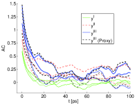
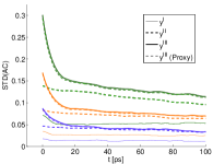
Figure 1: The AC of 4 realizations from 4 toy processes discussed in the text (left). The standard deviation of the AC curves measured in a trajectorywise fashion from a population of 100 trajectories. The computed standard deviation reflects the variance in a population of 100 empirically determined ACs.

In addition, a fourth process referred to as “III (Proxy)” will be evolved to demonstrate the AC method of Section III. This process is constructed by simply setting the parameters $\alpha^{0},\kappa^{0},\eta^{0}$ equal to the corresponding parameters of process III at time $t$ and then evolving this process like a standard OU model until the time index hits $t+\mathcal{T}$ when the parameters are updated to those of process III at the same time. This procedure is then iterated. Randomizing $\mathcal{T}$ had little influence on the accuracy here, but can be entertained. The processes above are simulated using the Euler-Maruyama scheme with time step size $\delta s$ and the process is observed discretely every $\delta t$ time unit. The remaining parameters are tuned to provide a parameter distribution consistent with those observed in some DHFR studies and are reported in the Appendix.

The toy model is used to investigate how variation induced by slowly evolving $\Gamma$ type factors influence the computed empirical AC on a controlled example where the assumptions behind the method introduced are satisfied. The features discussed are relevant to the DHFR system studied later and are also likely relevant to oher single-molecules studies. The example is also used to highlight issues relevant to nonergodic sampling klafter08 , i.e. when temporal averages are not equivalent to ensemble averages. In this type of situation, single-molecule data is particularly helpful. Use of the same Brownian motion term to drive three separate processes facilitates studying contributions to variance in these types of studies. In addition, estimation is not carried out to keep the discussion simple and to remove an additional source of uncertainty.

The left panel of Fig. 1 plots the empirical AC computed by sampling 4 realizations from this process using 5000 observations uniformly spaced by $\delta t=0.15ps$. These time series lengths are commensurate with those used in typical MD applications socci96 ; aroraAdK07 ; arora09 . One observes that the slowly evolving parameters do influence the AC measured. The fairly simple method of periodically updating the evolution parameters is able to mimic the AC associated with $y^{\mathrm{III}}$ for both short and long time scales. Furthermore, the variation induced by the relaxation and noise level (modulated by $\kappa_{t}$ and $\eta_{t}$) influences both the short time and longer time responses. The stochastic response of a dynamic disorder type process is clearly richer than a single exponential. An advantage the surrogate approach offers over popular existing methods for treating this situation socci96 is that other kinetic schemes, e.g. those associated with overdamped models with position dependent diffusion, can be entertained. In enzymes associated with complex dynamics, other kinetics schemes may be needed to accurately reflect the stochastic dynamics of the order parameter monitored. For example it is demonstrated in Fig. 3 that the PDOD surrogate is needed accurately captured relaxation kinetics even at short $O(ps)$ timescales. Over timescales relevant to experimentally accessible order parameters characterizing conformational fluctuations, one may need to account for dynamical responses much richer than a mixture of exponentials SPAJCTC ; karplus08 ; kou_08 . The procedure presented demonstrated how “elementary” pieces could be patched together to characterize relaxations/fluctuations occurring over longer timescales. This is attractive to both computer simulations and experimental data sets. In what follows the attention is shifted to focusing on limitations of using a single AC to describe single-molecule time series.

The right panel of Fig. 1 plots the standard deviation of the AC function associated with a trajectory population. For each observed trajectory, 100 different SDE trajectories were used to compute 100 empirical ACs from the time series associated with the trajectories. The pointwise standard deviation measured over the 100 ACs is plotted. The curve shadings distinguish different time series sample sizes. The three cases studied consisted of $(0.5,2,8)\times 10^{4}$ discrete temporal observations; each time series was uniformly sampled with $0.15ps$ between observations. Note that the influence of the evolving parameters on the measured AC is substantial. Recall all $y$ processes used common Brownian paths (so computer generated random numbers do not contribute to the differences observed). In addition, observe that the difference between $y^{\mathrm{II}}$ and $y^{\mathrm{III}}$ persists for a fairly long time and the length of time this difference is measurably noticeable depends on the temporal sample size used to compute the AC. In some applications, the variation induced by conformational fluctuations is important in computations gAIoan or to characterize a system AdK ; aroraAdK07 . The standard deviation in the measured AC here contains contributions coming from factors meant to mimic the influence unresolved conformational fluctuations whose influence persists for a fairly long time. In the AC computed with longer time series, i.e. spanning a larger time since the time between observations is fixed, the process has more time to “mix” and hence the difference between temporal and ensemble averages is reduced. Said differently, the influence of the initial conformation, or “memory”, diminishes. By using a single long time series trajectory and only reporting one AC computed from this “mixed” series, these types of physically relevant fluctuations can get washed out by using a single AC function. This goes against the spirit of single-molecule experiments.

The example considered here is admittedly simple and was constructed to illustrate the types of assumption behind the method introduced. If the dynamic disorder induced by large kinetic barriers or a complicated interaction with the surroundings, then one would need to construct more sophisticated processes for determining how and when the parameters regime switch. Combining the surrogate models with efforts along these lines, e.g. schuetteMMS09 , may be able to help these more exotic situations. Exploring the various routes by which complex and/or heavy tailed ACs xie04 ; kou_08 can emerge from simpler dynamical rules can help in a fundamental understanding of the governing physics granger80a ; granger80b ; cox91 ; klafter09 . However, if the ensemble average decay rate is deemed the only quantity of physical relevance then the collection of surrogate models can still potentially be used to help in roughly predicting the rate of decay of more complex ACs. This is particularly relevant to simulations where obtaining long enough trajectories to reliably calibrate models possessing complex AC exhibiting long range dependence from observed data is problematic Kaulakys_06 ; SPAJCTC ; kou_08 . Even in cases where one only requires the asymptotic time decay of an ensemble of conformations for a physical computation deshaw and can simulate for a long enough time to directly monitor kinetics, an understanding of the distribution of surrogate models estimated will likely be of help in linking computer simulation force fields to single-molecule experimental time series. The remaining results use simulations of DHFR to illustrate some of these points.

IV.2 Dihydrofolate Reductase(DHFR)

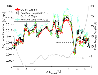
Figure 2: Average local diffusion function estimated (left axis) and free energy (right axis) as a function of order parameter. The population average of the estimated $C$ is plotted to give a feel for the position dependence of this quantity; it is stressed that the average alone is not adequate the describe the dynamics here due to a type of “dynamic disorder” phenomena xie_dynamicdis_98 . The free energy was computed by K. Arora using methods described in Ref. arora09 .

IV.2.1 DHFR Simulation Details

The detailed computational details are reported in Ref. arora09 . Briefly, an order parameter denoted by $\Delta D_{\mathrm{rmsd}}$, was defined using the root mean square distance between two crystal structures arora09 . This order parameter provides an indication of the proximity to the “closed” and “occluded” enzyme state and is reported in units of $\mathrm{\AA}$ throughout. The initial path between the closed and occluded conformations of DHFR was generated using the Nudged Elastic Band (NEB) method chu03 . Subsequently, $\approx$50 configurations obtained from NEB path optimization were subjected to US simulations. During these US simulations, production dynamics of 1.2$ps$ at 300K was performed after equilibration using a weak harmonic restraint.

IV.2.2 DHFR Results

Figure 2 plots the average local diffusion coefficient of the surrogate SDE models using two different observation frequencies on the left axis and on the right axis the free energy computed in Ref. arora09 is plotted. Each surrogate model was estimated using 400 time series observations with either $\delta=0.15$ or $\delta=0.30\ ps$ separating adjacent observations corresponding to $L=20$ or $L=10$ (respectively). The average local diffusion coefficient demonstrates a relatively smooth increasing trend for a majority of the order parameter values explored, but then suddenly changes abruptly around $\Delta D_{\mathrm{rmsd}}\approx 3\mathrm{\AA}$. It has been observed that an interesting interplay between free energy, fluctuations and stiffness, exists in some enzyme systems wolynes_crackingPNAS03 ; AdK ; wolynesHFSP08 ; Portman_CaMcracking09 and this plot suggests that future works investigating some of the finer structural factors leading to these change may be worthwhile, though this direction is left to future work because it is outside the scope of this study.

It is to be stressed that the mean of each US window is not adequate to summarize the dynamics. That is, a single fixed parameter surrogate SDE like the ones considered here cannot mimic the longer time statistics of the process. This is why the AC procedure introduced in Section III is needed. Figure 3 demonstrates that the individual PDOD models do capture features simpler surrogates cannot. This is due part to the position dependence of the local diffusion coefficient. The PDOD surrogate model combined with the procedure of Section III can accurately summarize the long time dynamics. These points are explained further in the discussion associated with Figs. 3-5.

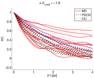
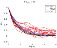
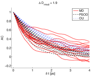
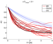
Figure 3: Local AC Function of MD data and that predicted by surrogates. The total time series of length 1.2 ns was divided into separate blocks, each containing 400 observations spaced by 0.15 ps. This data was used to estimate a collection of surrogate models and a collection of MD ACs corresponding to US target points of $\Delta D_{\mathrm{rmsd}}\approx-1.8,0.9,1.9$ and $3.1\mathrm{\AA}$. The AC corresponding to the estimate surrogate models is also plotted where the initial lag is normalized to unity to facilitate comparison (the raw units are shown in Fig. 3).

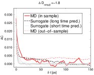
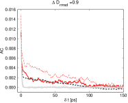
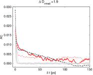
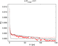
Figure 4: The global AC prediction. The procedure introduced here is used along with PDOD data to predict the long time AC. The relaxation predicted by the individual surrogate (data shown in Fig. 2 is also shown to stress that the SDE parameters are not fixed, but evolving and any single surrogate cannot capture the richer long time dynamics.

The ability of the PDOD model to capture features that a single exponential (e.g. the AC associated with an OU process) cannot is demonstrated in Fig. 3. Results from four different US points, each possessing a different degrees of position dependence on the noise are shown. Here the results obtained using both the OU and PDOD surrogates calibrated using the $\delta t=0.15ps$ with 400 temporal observations and the corresponding AC predictions are shown in the plot. The empirical ACs computed using the short segments of MD data used for surrogate model parameter estimation are also reported. Results with 400 blocks possessing observations spaced by $\delta t=0.30ps$ were similar in their AC prediction, but hypothesis tests strongly rejected the assumption of a fixed local diffusion (see Fig 5). The 400 $\delta t=0.15ps$ samples allowed the OU model structure to provide a better fit (as measured the fraction rejected) because the local diffusion function had less time to evolve/change value. For cases where the position dependence is moderate, the PDOD and OU surrogate models predict qualitatively similar AC functions. However, the PDOD model captures the short time relaxation dynamics better than the OU for cases where the position dependence of the local diffusion is more substantial and hence for clarity we focus on the PDOD models in the remaining kinetic studies.

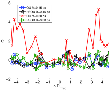
Figure 5: Goodness-of-fit tests. The test of Ref. hong was computed given the parameter estimate and the observed data. The median of each umbrella sampling window is reported.

Figure 4 plots the empirically determined AC obtained from different MD production simulation data. The case labelled “in-sample” was the one used for estimation of the local models reported in Fig. 3 and that labeled “out-of-sample” was computed by running a longer 3.6 ns simulation and computing the AC from the last 1.2 ns of this time series. The PDOD version of these models were used along with the procedure outlined in Section III using blocks of size 800 and randomizing the time index. The 400 blocks results were similar. Respecting the time ordering of the surrogate models only improved results marginally. Note also that the general trends of the long time decay of the MD data is captured with the procedure and that there is substantial difference between the “in-sample” and “out-of-sample” MD trajectories . The physical relevance of such variation was previously discussed and will be expanded on when results of stationary DHFR density prediction are shown. The primary observation is that a collection of PDOD surrogate models were able to capture the basic relaxation trends of the enzyme that a single surrogate could not. Recall that even at short timescales a single exponential decay was inadequate to fit the data. Similar trends were observed for all 51 US windows explored. However, it is to be stressed that the procedure shown here is to decompose kinetics in the longest contiguous block of discrete time series observed. If complex dynamics occur over longer timescales and data is not available that directly samples these scales, then the method cannot be used to predict the long time behavior that was not sampled.

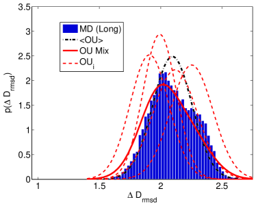
Figure 6: Stationary density/histogram prediction. The bars denote 1.2 $ns$ MD data, the solid thick line to the mixture PDOD method (see text), the solid dotted line to the average PDOD model, and the thin lines to the 4 local equilibrium densities used in constructing the mixture density.

The goodness-of-fit of the surrogate models using the two candidate SDEs is shown in Fig. 5 for various US windows. The median of the Q-test statistic introduced by hong is reported. This test statistic under the null is asymptotically normally distributed with mean zero and unit variance, but has also been proven to be useful in small samples hong ; molsim ; SPAJCTC ; gAIoan . Recall that each MD time series (at each umbrella sampling window) was divided into small pieces. In the portions near the edges (larger $|\Delta_{\mathrm{rmsd}}|$ values), where the position dependence of the noise is greatest, one observes that the OU model population has a median that would typically indicate a collection of poor dynamical models. If conformational fluctuations slowly modulate the dynamics, the longer the time series one has, the likelihood of departing from any simple surrogate model increases . Goodness-of-fit tests, like the one presented here, can be used to quantitatively approximate when simple models begin departing from various assumptions.

The stationary density predicted by the surrogate OU models in a case where position-dependence was shown to be marginal for the time interval data was monitored is plotted in Fig. 6. Here the mixture method discussed in Ref. SPAJCTC is reported due to its relevance to a collection of surrogates and dynamic disorder. The histogram of the $1.2ns$ MD data is also plotted as well as the stationary density predicted by a the average of the surrogate models taken at the US window near $\Delta D_{\mathrm{rmsd}}\approx 2$. Using a single model obtained by aggregating all time series together in hopes of reducing surrogate parameter uncertainty due to the resulting smaller time series sample sizes actually worsens the results. The mixture of OU models calibrated using 4 sets of noncontiguously spaced $60ps$ data (i.e. $400$ entries spaced $0.15ps$) were sampled every 300 ps from the MD process and this was used to compute 4 surrogate OU model parameters. The goodness-of-fit tests indicated that the local surrogates given the data were reasonable dynamical models. So portions where the “local equilibrium” density, i.e. the stationary density predicted by a surrogate with estimated parameters, possessing significant probability mass can be though of the regions of phase space sampled due to fast-scale motion for a relatively fixed (and unobserved) value of $\Gamma$ SPAJCTC ; SPAfilter . If variation in the conformational coordinate is important to thermodynamic averages, as the data here suggests to be the case in DHFR, then one needs to use a collection of “local equilibrium” densities SPAJCTC . The advantage of such an approach is that short bursts of simulations started from different initial conditions can be run, then surrogate models can be calibrated and tested. If the surrogate is found suitable, it can then be used to make predictions on the local equilibrium density, and the variation in the local equilibrium densities can be used to partially quantify the degree to which a slow conformational degree of freedom modulates the dynamics. This treatment is appealing when data on other physically relevant order parameters is unknown are not easy to access.

V Summary and Conclusions

Single-molecule experiments and simulations offer the potential for a detailed fundamental understanding of complex biomolecules without artifacts of bulk measurements obscuring the results. However, one must deal with complex multiscale fluctuations at this level of resolution and the factors contributing to the noise often contain physically relevant information such as quantitative information about conformational degrees of freedom SPAfilter . The abundance of data available to researchers and recent advances in computational and statistical methods are allowing researchers to entertain new methods of summarizing information relevant to modeling systems at the nanoscale SPAfilter ; SPAfric ; gAIoan .

By applying surrogate models to the data coming from biased MD simulations of DHFR, it was demonstrated that a collection of stochastic dynamical models can be used to better understand the factors contributing to the shape of the autocorrelation function associated with fluctuations coming from multiple time scales. The surrogate models were estimated by appealing to maximum likelihood type methods aitECO ; ozaki ; chen09 and were tested using goodness-of-fit tests which utilized the transition density of the assumed surrogate and were appropriate for the data. For example, the time series data was not assumed to be stationary; the stationarity assumption is often suspect in simulation data. The tests used hong indicated that taking the position dependence of the noise into account was required to provide a statistically acceptable model in many regions of phase space explored. For short timescales, the individual surrogate models (taking position dependence noise into account) were capable of predicting quantities outside of the fitting criterion, e.g. a parametric likelihood function was fit but the models were able to predict short timescale autocorrelation functions and these physically based models were able to fairly accurately summarize/model relaxation kinetics that a simple exponential relaxation could not. Other enzymes systems have exhibited this type of behavior SPAJCTC and it is likely that future single-molecule experiments will yield data possessing this feature.

Perhaps more importantly, we demonstrated that a population of surrogate models was required to represent the complex dynamical system because an unobserved conformational degree freedom modulated the dynamical response and this “random force” had to be accounted for in order to predict autocorrelations valid for longer temporal trajectories. A method using parametric surrogate models calibrated over short timescales while at the same time respecting the variability induced by unresolved coordinates evolving over longer timescale was presented. The DHFR system was another instance where aggregating a collection of simpler dynamical models gave rise to a more complex stochastic process granger80a ; granger80b ; cox91 ; SPAJCTC ; klafter09 . The basic idea is applicable to situations where a hidden slowly evolving degree of freedom modulates the dynamics and this coordinate evolves on an effective free energy surface possessing relatively low barriers SPAJCTC . Issues associated with extensions were briefly discussed.

Even if a coarse system description, such as a single autocorrelation function, can be used to adequately approximate the physically relevant statistical properties of all experimentally accessible observables, the approach presented still has appeal. One circumstance where this is particularly relevant is when computer simulation trajectories are compared to frequently sampled experimental single-molecule time series SPAfilter . In experimental time series, many conformational coordinates cannot typically be resolved SPAfilter ; SPAJCTC , so constructing a simulation that matches all relevant degrees of freedom is highly problematic. Quantitative knowledge of how the variability induced by such hidden degrees of freedom is reflected in the surrogate model parameters distribution may help in refining force fields to match kinetic properties at multiple timescales. If the force fields are believed valid, then turning to the simulations for details of the structural dynamics can help us in understanding complex molecular machines schultenscireview . This type of extra detail may also assist (or lead to new) methods for computing transition rates chandler00 . Furthermore, as nanotechnology demands higher resolution at smaller length and timescales, one may want to avoid using a single autocorrelation function constructed by aggregating many meso or microscopic states each possessing different dynamical features because doing so may unnecessarily wash out physically relevant information. The phenomenologically motivated simple bottom-up strategy presented was one contribution in this direction.

VI Acknowledgements

The author thanks Karunesh Arora and Charles Brooks III for sharing the DHFR data.

VII Appendix

VII.1 Toy Model Parameters

$\delta t=0.15,\delta s=\delta t/50,\mathcal{T}=200\times\delta t,\tau_{0}=120,(\alpha^{0},\kappa^{0},\eta^{0})=(4,0.2,0.5),(\sigma^{\alpha},\sigma^{\kappa},\sigma^{\eta})=(6.5\times 10^{-2},6.5\times 10^{-3},1.9\times 10^{-2})$. The last set of parameters were selected to give the evolving OU parameters a stationary distribution characterized by three independent normals each having mean $(\alpha^{0},\kappa^{0},\eta^{0})$ and standard deviation (1/2,1/20, 3/20). The initial condition of each $y$ process was set to $\alpha^{0}$ and the OU parameters were all set to $(\alpha^{0},\kappa^{0},\eta^{0})$. 100 batches of 4 independent Brownian motion processes were used to evolve the system.

VII.2 Predicting Quantities with Surrogate Models

The OU process is attractive for a variety of reasons. Its conditional and stationary density are both known analytically and it can be readily estimated from discrete data. For parameters possessing a stationary distribution, these can all be written explicitly in terms of Normal densities. Another appealing feature is that the AC function, denote this function by $AC(t)$, [28] associated with a stationary process can readily be computed after parameter estimates are in hand, namely $AC(t)=\exp{-Bt}$; recall the drift of the OU process is given by $B(A-z)$.

Unfortunately, these types of statistical summaries are more difficult to obtain with other SDEs. Position dependence of the diffusion function and nonlinear models severely complicate obtaining analytic expressions for the autocorrelation function. Note that once a single SDE models is estimated, a new large collection of sample paths can be simulated and quantities like the autocorrelation function associated with a given SDE model and $\theta$ can be empirically determined (the computational cost of simulating a scalar SDE is typically marginal in relation to a MD simulation). This can be repeated for each surrogate SDE estimated from each MD path.

However, a stationary density, under mild regularity conditions, of a scalar SDE can often be expressed in closed-form using only information contained in the estimated SDE coefficient functions via the relation [55, 40]

$$p^{SD}(z;\Gamma)=\mathcal{Z}/\sigma(z)^{2}\exp\Big{(}\int^{z}_{z_{\mathrm{REF}}}\mu(z^{\prime})/\sigma(z^{\prime})^{2}dz^{\prime}\Big{)},$$ (5)

where in the above the SDE functions’ dependence on $\theta$ and $\Gamma$ has been suppressed to streamline the notation. $\mathcal{Z}$ represents a constant to ensure that the density integrates to unity and $z_{\mathrm{REF}}$ represents an arbitrary fixed reference point. When evaluating $p^{SD}(\cdot)$, one can encounter technical difficulties if the diffusion coefficient is allowed to take a zero or negative value (this is relevant to the PSOD model). Some heuristic computational approaches to dealing with this are discussed in Refs. [44, 13].

Sometimes a thermodynamic motivation exists for expressing the stationary density of the high-dimensional molecular system in terms of some potential, denoted here by $V(z)$, that does not explicitly depend on the diffusion function [40, 39]. In time-homogeneous scalar overdamped Brownian dynamics, where the forces of interest acting on $z$ are believed related to the gradient of $V(z)$, a “noise-induced drift” term [40] can be added to the drift function and this addition cancels out the contribution coming from the $1/\sigma(z)^{2}$ term outside the exponential. The stationary density of the modified SDE can then be expressed as being proportional to $\exp{\big{(}-V(z)\big{)}}$ in such a situation. This type of modification has a thermodynamic appeal when $z$ is the only important variable of the system and the fast-scale noise has been appropriately dealt with [38]. The utility of such an approach in describing the pathwise kinetics of trajectories is another issue and single-molecule studies are one area where the distinction may be important (one may not care as much about the stationary ensemble distribution) .

However when there are slowly evolving lurking variables like $\Gamma$ modulating the dynamics (as is the case in many biomolecular systems) using simple expression like Eq. 5 to approximate the stationary density of the high-dimensional system (with or without “noise-induced drift” corrections) is highly problematic. Note that the $\Gamma$ variable has been retained in the left hand side of Eq. 5; the stationary density estimate is only meant to be valid for a fixed estimated SDE surrogate corresponding to one value $\theta$. In this paper and others, it is assumed that for a short time interval both $\theta$ and $\Gamma$ are effectively frozen. Given a model and short time data, this can be tested using goodness-of-fit tests. However over longer timescales, $\Gamma$ evolves and modulates the dynamics so the estimated $\theta$ evolves in time (this is why the situation can be though of as a type of dynamic disorder [1]). For this long time evolution, it is assumed that the form of a stochastic process depending only on $z$ is completely unknown to the researcher. Furthermore it was assumed that another order parameter (i.e. system observable) is unavailable or is unknown [13, 26, 48]. Hence to approximate the stationary distribution of the high-dimensional molecular system one would require a collection of $p^{SD}$’s (each with different $\Gamma$’s) to approximate this quantity. This procedure is presented in Ref. [13].

References

- [1] H.P. Lu, L. Xun, and X.S. Xie. Single-molecule enzymatic dynamics. Science, 282:1877–1881, 1998.
- [2] S.C. Kou and X.S. Xie. Generalized Langevin equation with fractional Gaussian noise: Subdiffusion within a single protein molecule. Phys. Rev. Lett., 93:180603, 2004.
- [3] M. Vendruscolo and C. M. Dobson. Dynamic visions of enzymatic reactions. Science, 313:1586, 2006.
- [4] K.A. Henzler-Wildman and et al. Intrinsic motions along an enzymatic reaction trajectory. Nature, 450:06410, 2007.
- [5] O. Miyashita, J. N. Onuchic, and P. G. Wolynes. Nonlinear elasticity, proteinquakes, and the energy landscapes of functional transitions in proteins. Proc. Natl. Acad. Sci. U.S.A., 100:12570–12575, Oct 2003.
- [6] C.P. Calderon and K. Arora. Extracting kinetic and stationary distribution information from short md trajectories via a collection of surrogate diffusion models. J. Chem. Theory Comput., in press.
- [7] P. C. Whitford, J. N. Onuchic, and P. G. Wolynes. Energy landscape along an enzymatic reaction trajectory: hinges or cracks? HFSP J, 2:61–64, Apr 2008.
- [8] K. Arora and C. L. Brooks Iii. Functionally Important Conformations of the Met20 Loop in Dihydrofolate Reductase are Populated by Rapid Thermal Fluctuations. J. Am. Chem. Soc., Mar 2009.
- [9] J. P. Junker, F. Ziegler, and M. Rief. Ligand-dependent equilibrium fluctuations of single calmodulin molecules. Science, 323:633–637, 2009.
- [10] S. Tripathi and J. J. Portman. Inherent flexibility determines the transition mechanisms of the EF-hands of calmodulin. Proc. Natl. Acad. Sci. U.S.A., 106:2104–2109, Feb 2009.
- [11] C.P. Calderon. On the use of local diffusion for path ensemble averaging in potential of mean force computations. J. Chem. Phys., 126:084106, 2007.
- [12] C.P. Calderon and R. Chelli. Approximating nonequilibrium processes using a collection of surrogate diffusion models. J. Chem. Phys., 128:145103, 2008.
- [13] C.P. Calderon and K. Arora. Extracting kinetic and stationary distribution information from short md trajectories via a collection of surrogate diffusion models. J. Chem. Theory & Comput., 5:47, 2009.
- [14] Ariel Lubelski, Igor M. Sokolov, and Joseph Klafter. Nonergodicity mimics inhomogeneity in single particle tracking. Physical Review Letters, 100(25):250602, 2008.
- [15] S. Kou. Stochastic modeling in nanoscale biophysics: subdiffusion within proteins. Annals of Applied Statistics, 2:501–535, 2008.
- [16] G. Hummer. Position-dependent diffusion coefficients and free energies from Bayesian analysis of equilibrium and replica molecular dynamics simulations. New J. Phys., 7:34, 2005.
- [17] J. Chahine, R.J. Oliveira, V.B.P. Leite, and J. Wang. Configurational-dependent diffusion can shift the kinetic transition state and barrier height of protein folding. Proc. Natl. Acad. Sci. USA, 104:14646, 2007.
- [18] Y. Aït-Sahalia. Maximum-likelihood estimation of discretely-sampled diffusions: A closed-form approximation approach. Econometrica, 70:223–262, 2002.
- [19] J.C. Jimenez and T. Ozaki. An approximate innovation method for the estimation of diffusion processes from discrete data. J. Time Series Analysis, 27:77–97, 2006.
- [20] S. Chen and Tang C.Y. Parameter estimation and bias correction for diffusion processes. J. Econometrics, 149:65–81, 2009.
- [21] Y. Pokern, A.M. Stuart, and E. Vanden-Eijnden. Remarks on drift estimation for diffusion processes. Multiscale Model. Simul., in press, 2009.
- [22] C.P. Calderon. Fitting effective diffusion models to data associated with a “glassy potential”: Estimation, classical inference procedures and some heuristics. Mutliscale Modeling and Simulation, 6:656–687, 2007.
- [23] Yacine Ait-Sahalia, Jianqing Fan, and Heng Peng. Nonparametric transition-based tests for jump-diffusions. JASA, in press, 2009.
- [24] S.X. Chen and C.Y. Tang. A test for model specification of diffusion processes. Annals of Statistics, 36:167–198, 2008.
- [25] Y. Hong and H. Li. Nonparametric specification testing for continuous-time models with applications to term structure of interest rates. The Review of Financial Studies, 18:37–84, 2005.
- [26] C.P. Calderon, N. Harris, C.-H. Kiang, and D.D. Cox. Quantifying multiscale noise sources in single-molecule time series via pathwise statistical inference procedures. J. Phys. Chem. B, 113:138, 2009.
- [27] C.P. Calderon, W.-H. Chen, N. Harris, K.J. Lin, and C.-H. Kiang. Analyzing DNA melting transitions using single-molecule force spectrscopy and diffusion models. J. Physics: Condensed Matter, 21:034114, 2009.
- [28] N. D. Socci, J. N. Onuchic, and P. G. Wolynes. Diffusive dynamics of the reaction coordinate for protein folding funnels. J. Chem. Phys., 104:5860–5868, 1996.
- [29] C. W. J. Granger. Long memory relationships and the aggregation of dynamic models. Journal of Econometrics, 14(2):227 – 238, 1980.
- [30] C.W.J. Granger and R. Joyeux. An introduction to long-memory time series models and fractional differencing. J. Time Series. Analysis, 1:15–30, 1980.
- [31] D.R. Cox. Long-range dependence, non-linearity and time irreversibility. J. Time Series. Analysis, 12:329–335, 1991.
- [32] Iddo Eliazar and Joseph Klafter. From ornstein-uhlenbeck dynamics to long-memory processes and fractional brownian motion. Physical Review E (Statistical, Nonlinear, and Soft Matter Physics), 79(2):021115, 2009.
- [33] B.L.S. Prakasa Rao. Statistical Inference for Diffusion Type Processes. Hodder Arnold, 1999.
- [34] C.P. Calderon, L. Janosi, and I. Kosztin. Using stochastic models calibrated from nanosecond nonequilibrium simulations to approximate mesoscale information. J. Chem. Phys., 130:144908, 2009.
- [35] R. Zwanzig. Nonequilibrium Statistical Mechanics. Oxford University Press, New York, 2001.
- [36] C.W. Gardiner. Handbook of Stochastic Models. Springer-Verlag, Berlin, 1985.
- [37] S. Park and K. Schulten. Calculating potentials of mean force from steered molecular dynamics simulations. J. Chem. Phys., 120:5946–5961, 2004.
- [38] R. Kupferman, , G.A. Pavliotis, and A.M. Stuart. Ito versus stratonovich white noise limits for systems with inertia and colored multiplicative noise. Phys. Rev. E, 70:036120, 2004.
- [39] D.I. Kopelevich, A.Z. Panagiotopoulos, and I.G. Kevrekidis. Coarse-grained kinetic computations for rare events: Application to micelle formation. J. Chem. Phys., 122:044908, 2005.
- [40] H. Risken. The Fokker-Planck Equation. Springer-Verlag, 1996.
- [41] Peter Arnold. Langevin equations with multiplicative noise: Resolution of time discretization ambiguities for equilibrium systems. Phys. Rev. E, 61(6):6091–6098, Jun 2000.
- [42] Cristian Micheletti, Giovanni Bussi, and Alessandro Laio. Optimal langevin modeling of out-of-equilibrium molecular dynamics simulations. The Journal of Chemical Physics, 129(7):074105, 2008.
- [43] G. Hummer and A. Szabo. Free energy reconstruction from nonequilibrium single-molecule pulling experiments. Proc. Natl. Acad. Sci. USA, 98:3658–3661, 2001.
- [44] C.P. Calderon. Local diffusion models for stochastic reacting systems: estimation issues in equation-free numerics. Mol. Sim., 33:713–731, 2007.
- [45] C.P. Calderon, N. Harris, C.-H. Kiang, and D.D. Cox. Analyzing single-molecule manipulation experiments. J. Mol. Recognit., in press, 2009.
- [46] P. Kloeden and E. Platen. Numerical Solution of Stochastic Differential Equations. Springer-Verlag, 1992.
- [47] K. Arora and C. L. Brooks, III. Large-scale allosteric conformational transitions of adenylate kinase appear to involve a population-shift mechanism. Proc. Natl. Acad. Sci. USA, 104:18496–18501, 2007.
- [48] S. V. Krivov and M. Karplus. Diffusive reaction dynamics on invariant free energy profiles. Proc. Natl. Acad. Sci. U.S.A., 105:13841–13846, Sep 2008.
- [49] I. Horenko and Schutte C. Likelihood-based estimation of multidimensional langevin models and its application to biomolecular dynamics. Mult. Mod. Sim., in press.
- [50] Nonlinear stochastic models of 1/f noise and power-law distributions. Physica A: Statistical Mechanics and its Applications, 365(1):217 – 221, 2006.
- [51] P. Maragakis, K. Lindorff-Larsen, M.P. Eastwood, R.O. Dror, J.L. Klepeis, I.T. Arkin, M.O. Jensen, H. Xu, N. Trbovic, R.A. Friesner, A.G. Palmer, and D.E. Shaw. Microsecond molecular dynamics simulation shows effect of slow loop dynamics on backbone amide order parameters of proteins. J. Phys. Chem. B, 112:6155–6158, 2008.
- [52] Jhih-Wei Chu, Bernardt L. Trout, and Bernard R. Brooks. A super-linear minimzation scheme for the nudged elastic band method. J. Chem. Phys., 119(24):12708–12717, 2003.
- [53] M. Sotomayor and K. Schulten. Single-molecule experiments in vitro and in silico. Science, 316:1144 – 1148, 2007.
- [54] P. G. Bolhuis, C. Dellago, and D. Chandler. Reaction coordinates of biomolecular isomerization. Proc. Natl. Acad. Sci. U.S.A., 97:5877–5882, May 2000.
- [55] Y.A. Kutoyants. Statistical Inference for Ergodic Diffusion Processes. Springer, New York, 2003.