Faint Lyman-Break galaxies as a crucial test for galaxy formation models

Abstract

It has recently been shown that galaxy formation models within the $\Lambda$CDM cosmology predict that, compared to the observed population, small galaxies (with stellar masses $<10^{11}$ M_⊙) form too early, are too passive since $z\sim 3$ and host too old stellar populations at $z=0$. We then expect an overproduction of small galaxies at $z\ga 4$ that should be visible as an excess of faint Lyman-break galaxies. To check whether this excess is present, we use the morgana galaxy formation model and grasil spectro-photometric $+$ radiative transfer code to generate mock catalogues of deep fields observed with HST-ACS. We add observational noise and the effect of Lyman-alpha emission, and perform color-color selections to identify Lyman-break galaxies. The resulting mock candidates have plausible properties that closely resemble those of observed galaxies. We are able to reproduce the evolution of the bright tail of the luminosity function of Lyman-break galaxies (with a possible underestimate of the number of the brightest $i$-dropouts), but uncertainties and degeneracies in dust absorption parameters do not allow to give strong constraints to the model. Besides, our model shows a clear excess with respect to observations of faint Lyman-break galaxies, especially of $z_{850}\sim 27$ $V$-dropouts at $z\sim 5$. We quantify the properties of these “excess” galaxies and discuss the implications: these galaxies are hosted in dark matter halos with circular velocities in excess of 100 km s^-1, and their suppression may require a deep re-thinking of stellar feedback processes taking place in galaxy formation.

1 Introduction

Despite the large observational and theoretical efforts of the last decade, the formation of galaxies in the context of the $\Lambda$CDM cosmology is still an open problem. In fact, the wealth of multi-wavelength data on deep fields, coupled with wide local surveys, has produced new constraints on number densities, stellar masses, star formation rates and metallicities of galaxies in the redshift range from 0 to $\sim 7$. From the phenomenological point of view, a remarkable behaviour of observed galaxies is their “downsizing” trend in star formation rates, stellar masses, chemical enrichment, reconstructed age of stellar populations, reconstructed duration of the main star formation episode (see references in Fontanot et al., 2009). For “downsizing” here we mean that more massive galaxies tend to be older than less massive ones in terms of either stellar ages or mass assembly, a behaviour that is at variance with that of dark matter halos.

These constraints are a strong challenge to theoretical models of galaxy formation. In a recent paper, Fontanot et al. (2009) compared the predictions of three galaxy formation models (Wang et al., 2008; Monaco et al., 2007; Somerville et al., 2008) with observational data which showed downsizing trends. This analysis allowed the authors to highlight a significant discrepancy between models and data that pertains to relatively small galaxies, with stellar masses in the range $10^{9}-10^{10.5}$ M_⊙. In all three models these galaxies are formed at high redshift and are rather old and passive at late times, while the population of real galaxies in the same stellar mass range builds up at low $z$, growing in number by a factor of $\sim 3$ from $z\sim 1$ to the present time, and shows higher specific star formation rates up to $z\sim 3-4$. Similar conclusions are obtained considering the age of stellar populations in local galaxies: real galaxies host much younger stars on average than model galaxies. The consistency of results coming from stellar masses, star formation rates and reconstructed stellar ages makes this trend robust. Previous comparisons, focused on stellar mass downsizing, showed that this discrepancy is not limited to the three models tested in that paper but extends to many semi-analytic and N-body codes (see the comparisons to models in Fontana et al., 2006; Cirasuolo et al., 2008; Marchesini et al., 2008).

This is a severe discrepancy because, as we will discuss later in this paper, it cannot be easily solved by a simple fine-tuning of parameters. Also, it is not directly related to the well-known tendency of semi-analytic models to produce steep luminosity functions, because all the model stellar mass functions have roughly the correct slope at $z=0$, or to the well-known problem of overquenching of satellite galaxies, which are too red and passive in models (see, e.g., the recent analysis of Kimm et al., 2008). Clearly the solution of this problem amounts to understanding why do small galaxies form so early and why do they stop forming stars later. The second problem is most likey a byproduct of the first one: once too many small galaxies are produced at high redshift, strong stellar feedback must be invoked to suppress their star formation at lower redshift, so as to recover the correct number density at $z=0$. Then, the crucial objects that are at the origin of this discrepancy are the small star-forming galaxies at $z>3$. Unfortunately, with presently available facilities only the rest-frame UV radiation of such galaxies is accessible; these are visible as distant faint Lyman-break galaxies. Their name takes origin from the technique used to select them, also known as “dropout technique”. This technique selects galaxies over a specific redshift interval by detecting the drop of the UV flux observed in correspondence with the Lyman limit at $\lambda$ $<$ 912 Å, the wavelength below which the ground state of neutral hydrogen may be ionized.

In this paper we use the morgana + grasil model of galaxy formation to generate predictions of $B$-, $V$- and $i$-dropouts to be compared with the results of (i) the GOODS-S photometric and spectroscopic data by Giavalisco et al. (2004) and Vanzella et al. (2008), (ii) the GOODS-MUSIC sample (Grazian et al., 2006) with photometric redshifts, (iii) the results of Bouwens et al. (2007), where many HST-ACS deep fields were analysed and scaled to the depth of the Hubble Ultra Deep Field (HUDF, Beckwith et al., 2006).

Several previous theoretical studies addressed the properties of Lyman-break galaxies using both semi-analytical models (Somerville et al., 2001; Poli et al., 2001, 2003; Blaizot et al., 2004; Baugh et al., 2005; Mao et al., 2007; Gao et al., 2008; Overzier et al., 2008; Lee et al., 2008; Guo & White, 2008) and cosmological simulations (Nagamine, 2002; Weinberg et al., 2002; Harford & Gnedin, 2003; Nagamine et al., 2004; Finlator et al., 2006; Night et al., 2006; Nagamine et al., 2008). These papers checked how models within the $\Lambda$CDM cosmology are able to reproduce the properties of Lyman-break galaxies and their clustering, often reporting satisfactory agreement. Despite some authors (namely Poli et al., 2001, 2003; Night et al., 2006; Finlator et al., 2006) noticed that models tend to overproduce faint high-redshift Lyman Break Galaxies with respect to observations, no quantitative claim had been possible at that time, given the uncertainties on the observational constraints. As an example, Finlator et al. (2006) found that their predicted steep faint-ends of the luminosity function were still in agreement with the available data, which spanned a range of values from $-2$.2 to $-1.6$. This wide range has recently been revised by (Bouwens et al., 2007), so that the most recent determinations give a slope $\sim 1.7\pm 0.1$ from $z\sim 2$ to $z\sim 6$, which implies a disagreement with the theoretical predictions.

The aim of this paper is a careful revision of this comparison, in the light of the improved observational constraints, based on the generation of reliable and improved mock galaxy catalogues through state-of-the-art semi-analytical and spectro-photometric models. This approach will allow us to test the impact of the selection criteria, as well as different theoretical ingredients (with particular emphasis on the modeling of dust attenuation). Moreover, we aim to include this comparison in a cosmological context, and to discuss its implications for current models of galaxy formation and the so-called ”downsizing” scenario (see e.g. Fontanot et al. (2009)).

The plan of the paper is the following. Section 2 presents the model, which contains some improvements with respect to previous versions. Section 3 describes the adopted procedure to select Lyman-break galaxies from the simulated galaxy catalogues and to tune the free parameters connected to dust extinction. Section 4 presents the comparison of model and data in terms of number counts, redshift and color distributions and luminosity functions of $B$,$V$ and $i$-dropouts, while Section 5 quantifies the properties of the model “excess” galaxies and discusses future observational tests that can help shedding light on this population. Section 6 gives the conclusions.

2 The morgana + grasil model

2.1 morgana

The MOdel for the Rise of GAlaxies aNd Agns (morgana) is described in full detail in Monaco et al. (2007). The model follows the general scheme of semi-analytic models (see Baugh, 2006, for a review); here we only mention how the main processes are implemented. (i) Each dark matter halo hosts a central galaxy and many satellite galaxies, contained within dark matter substructure that has not yet been destroyed by orbital decay due to dynamical friction. Baryons are subdivided into stellar halo, bulge and disc components. Each component has cold, hot and stellar phases. (ii) Merger trees of dark matter halos are obtained using the pinocchio tool (Monaco et al. 2002; Monaco, Theuns & Taffoni 2002; Taffoni et al. 2002). (iii) After a merging of dark matter halos, galaxy merging times are computed using the results of Taffoni et al. (2003), which are tuned on N-body simulations that include dynamical friction, tidal stripping and tidal shocks. (iv) At each merger a fraction of the satellite stellar mass is moved to the diffuse stellar component of the stellar halo, as explained in Monaco et al. (2006). (iv) The evolution of the baryonic components and phases is performed by numerically integrating a system of equations for all the mass, energy and metal flows. (v) The intergalactic medium infalling on a dark matter halo is shock-heated to a specific thermal energy equal to 1.2 times that of dark matter. (vi) At each time-step of the numerical integration, the hot gas component is assumed to be in hydrostatic equilibrium with the dark matter halo. (vii) Cooling flows are computed with a new cooling model, tested against simulations of isolated halos in Viola et al. (2008), which takes into account mass and energy input from feedback sources. (viii) The cooling gas is let infall on the central galaxy on a dynamical time-scale. It is divided between disc and bulge according to the fraction of the disc that lies within the half-mass radius of the bulge. (ix) The gas infalling on the disc keeps its angular momentum; disc sizes are computed with an extension of the Mo, Mao & White (1998) model that includes the contribution of the bulge to the disc rotation curve. (x) Disc instabilities and major mergers of galaxies lead to the formation of bulges. In minor mergers the satellite mass is given to the bulge component of the larger galaxy. (xi) Star formation and feedback in discs are inserted following the model of Monaco (2004), while in bulge components the Kennicutt (1998) law is used. In both cases, hot gas is ejected to the halo (in a hot galactic wind) at a rate equal to the star-formation rate. (xii) Feedback from star formation heats the hot halo phase. When its temperature gets significantly higher than the virial one, it leaves the dark matter halo in a galactic hot super-wind. The matter is re-acquired later, when the virial temperature of the descendant halo gets as high as that of the hot superwind gas. (xiii) In star-forming bulges cold gas is ejected in a cold galactic wind by kinetic feedback due to the predicted high level of turbulence driven by SNe. Analogously to the hot superwind, cold halo gas can be ejected out of the dark matter halo if its kinetic energy is high enough. (xiv) Accretion of gas onto massive black holes (starting from small seeds present in all galaxies) is connected to the ability of cold gas to loose angular momentum by some (unspecified) mechanisms driven by star formation. This is explained in full detail in Fontanot et al. (2006). (xv) The kind of feedback from the AGN depends on the accretion rate in Eddington units: whenever this is higher than 1 per cent the AGN can trigger a massive galaxy wind, (see Monaco & Fontanot, 2005) which leads to the complete removal of Inter-Stellar Medium (ISM) from the galaxy, while at lower accretion rates the energy is ejected through jets that feed back on the hot halo gas; this can lead to quenching of the cooling flow.

2.2 The improvements with respect to the earlier version

The version of the model used here presents a few improvements with respect to that of Monaco et al. (2007). The most important difference lies in the treatment of star formation in the bulge component. In the earlier version, the size of the starburst, used to compute the gas surface density and then the star formation rate through the Kennicutt (1998) relation, was assumed to be equal to the bulge effective radius $R_{b}$. As a consequence, a starburst declines very slowly because the residual gas has a decreasingly low surface density, and then a long star formation time-scale. This is a clearly naive estimate, because the dissipational gas settles in the centre of the galaxy. In this version we assume that the size of the starburst is determined by the level of turbulence that the gas acquires. The velocity dispersion $\sigma_{\rm cold}$ due to turbulence is:

$$\sigma_{\rm cold}=\sigma_{0}\left(\frac{t_{\star}}{1\ {\rm Gyr}}\right)^{-1/3}$$ (1)

where the parameter $\sigma_{0}$ is set to 60 km s^-1. Fontanot et al. (2006) show that this value allows a good reproduction of the evolution of the AGN population. The time-scale of star formation $t_{\star}$ is:

$$t_{\star}=4\;\left(\frac{\Sigma_{\rm cold}}{1\ {\rm M}_{\odot}\ {\rm pc}^{-2}}\right)^{-0.4}\ {\rm Gyr}$$ (2)

where $\Sigma_{\rm cold}$ is the (cold) gas surface density. The size of the startburst is determined as the radius for which the turbulence-driven velocity dispersion equals that of the host bulge computed at the same radius. For the Young mass profile used in the model, the bulge velocity curve is roughly constant (assuming a value $\sim 0.707V_{\rm bulge}$, where $V_{\rm bulge}$ is the circular velocity of the bulge) down to 0.04 times the effective radius $R_{b}$, where it quickly drops to zero. Consequently, the size of starbursts in bulges is estimated as:

$$R_{\rm gas}=\left(\frac{\sigma_{\rm cold}(R_{b})}{0.707V_{b}}\right)^{3.75}R_{b}$$ (3)

where $\sigma_{\rm cold}(R_{b})$ is computed using $R_{b}$ to determine the surface density (equation 2). The radius $R_{\rm gas}$ is not allowed to be smaller than $0.04R_{b}$.

A second difference is that we optimized this version of the model for a Chabrier (2003) mass function instead of the Salpeter one used before. To achieve the same level of agreement with data as with Salpeter we perform the following parameter changes (please refer to Monaco et al. (2007) for all details): (i) the stellar mass per supernova is $M_{\rm\star,SN}=84$ M_⊙, the restoration rate is $f_{\rm rest}=0.44$, while the metal yield per generation is set to $Y=0.016$; (ii) the preferred values of some parameters change to: $n_{\rm quench}=0.3$, $n_{\rm dyn}=0.3$, $f_{\rm wind}=2.0$, $f_{\rm th,B}=0.1$, $f_{\rm th,D}=0.32$, $f_{\rm jet,0}=3.0$. Quasar-triggered galaxy winds are present as in Fontanot et al. (2006); dark matter halo concentrations are not rescaled to improve the fit of the baryonic Tully-Fisher relation. Moreover, the threshold for disc instability is relaxed from $\epsilon_{\rm limit}=0.9$ to 0.7; this allows to remove the excess of small bulges present in the previous version of the model (see Figure 7 of Monaco et al., 2007).

Finally, to slow down the merger-driven evolution of the most massive galaxies, at each merger a fraction $f_{\rm scatter}=0.8$ of the stellar mass of each satellite is given to the halo diffuse stellar component; however, this is done only at $z<1$, as suggested by Conroy et al. (2007). This is not a physically acceptable solution of the problem raised by Monaco et al. (2006), but has the advantage of giving realistic results.

2.3 grasil

For each galaxy modeled by morgana the corrisponding UV-to-radio SED is computed with the spectro-photometric $+$ radiative transfer code grasil (Silva et al., 1998, please refer to this paper for a detailed description of this code). According to this model, stars and dust are distribuited in a bulge (King profile) + disc (radial and vertical exponential profiles) axisymmetric geometry. Three different dusty environments are taken into account: (1) dust in interstellar HI clouds heated by the general interstellar radiation field of the galaxy (the “cirrus” component), (2) dust associated with star-forming molecular clouds and HII regions, and (3) circumstellar dust shells produced by the windy final stages of stellar evolution. These environments have different importance in different galactic systems at various evolutionary stages. Therefore the residual gas fraction in the galaxy is divided into two phases: the dense giant molecular clouds (MCs) and the diffuse medium (“cirrus”). The fraction of gas in the molecular phase, $f_{\rm mol}$, is a model parameter. The molecular gas is subdivided into clouds of given mass and radius: the stars are assumed to be born within the optically thick MCs and gradually to escape from them, as they get older, on a time-scale $t_{\rm esc}$. To compute the emitted spectrum of the star-forming molecular clouds a radiative transfer code is used. The diffuse dust emission is derived by describing the galaxy as an axially symmetric system, in which the local dust emissivity is consistently computed as a function of the local field intensity due to the stellar component.

For each galaxy modelled by morgana, star formation histories, together with gas and metal contents at the “observation” time for both bulge and disc component, are then given as an input to grasil. Unobscured stellar SEDs are generated by using again a Chabrier (2003) IMF with stellar masses in the limit [0.15-120] M_⊙. In the radiative transfer computation the effect of dust is limited to absorption; dust emission, which is very expensive from the point of view of computational time, is irrelevant in the rest-frame UV spectral regions sampled here. Absorption from the Inter-Galactic Medium (IGM) is taken into account by applying to the redshifted SEDs the Madau (1995) attenuation, as explained in Fontanot et al. (2007).

Here below the grasil parameters that are not provided by MORGANA and which play an important role in the dust parametrization are briefly discussed. We also recall the values used in Fontanot et al. (2007) to compare with $K$-band and sub-mm selected galaxies.

(i) $t_{esc}$ represents the time-scale for young O-B stars to escape from their parent MCs. In Fontanot et al. (2007) we fixed the value of $t_{esc}$ to $10^{7}yr.$. This is an intermediate value between those found by Silva et al. (1998) to well describe the SED of spirals ($\sim$ a few Myr) and starburst ($\sim$ a few 10 Myr), and it is of the order of the estimated destruction time-scale of MCs by massive stars. (ii) The cold gas mass provided by MORGANA is subdivided between the dense and diffuse phases. In Fontanot et al. (2007) we fixed the fraction of gas in MCs $f_{\rm mol}$ to $0.5.$. (iii) The total (i.e., cirrus + MCs) dust content of a galaxy ISM is obtained by the residual gas mass and the dust-to-gas mass ratio $\delta$ which is assumed to scale linearly with the metallicity ($\delta=0.45Z$). The optical depth of MCs depends on their mass and radius only through the relation $\tau\propto\delta M_{MC}/r^{2}_{MC},$. In Fontanot et al. (2007) we assumed $M_{MC}=10^{6}M_{\odot}$, $r_{MC}=16pc$. (iv) The bulge and disc scale radii for stars and gas are given by MORGANA, while the disc scale-heights, $h^{*}_{d}$ and $h^{d}_{d}$ for stars and dust, respectively, are set as in Fontanot et al. (2007) to $0.1$ the corresponding scale radii. The dust grain size distribution and abundances are set so as to match the mean Galactic extinction curve and emissivity as in Silva et al. (1998) and Vega et al. (2005) and are not varied here.

Because the rest-frame UV emission is especially sensitive to dust attenuation, there is no guarantee that the parameters used in Fontanot et al. (2007) are suitable for Lyman-break galaxies (see Fontanot et al., 2009, for a discussion on dust attenuation at low and high redshift). In this paper we will explore the effect of changing the values of the two parameters $t_{esc}$ and $f_{mol}$ keeping fixed the other ones. These parameters, in fact, by definition, are those which can play a fundamental role in the attenuation of the UV emission from young massive stars. This will be discussed in more detail in the next section.

2.4 Lyman-$\alpha$ emission line

Many Lyman-break galaxies show a prominent Lyman-$\alpha$ emission line, which may influence galaxy colors. This is especially true at the highest redshift, where the $i$-$z$ color can get significantly bluer, so that the selection of a galaxy as an $i$-dropout is shifted to higher redshift. Modeling the effect of such emission is very difficult due to the resonant scattering of Lyman-$\alpha$ photons by neutral hydrogen which implies that even a small amount of dust is sufficient to absorb many emitted photons and attenuate the Lyman-$\alpha$ line. The observed lines are generally ascribed to the presence of galactic winds which allow Lyman-$\alpha$ photons to escape the galaxy after a few scatterings. Radiative transfer calculations of Lyman-$\alpha$ through winds have shown that this process can explain the observed asymmetric line profiles (e.g. Shapley et al., 2003; Vanzella et al., 2006; Verhamme et al., 2008). Due to this complexity, we prefer to make an empirical estimate of the possible influence of the Lyman-$\alpha$ line on galaxy colors and number counts.

To this aim, we add a Lyman-$\alpha$ emission line to the produced spectra, with specified $EW$. Given the relatively coarse wavelength sampling used (sufficient to compute magnitudes over standard filters), this line is added to one single wavelength bin. With the VLT/FORS2 spectroscopic campaign of the GOODS-S field the number of Lyman-break candidates with observed Lyman-$\alpha$ emission lines is 25 over 85 for the $B$-dropouts, 19 over 52 for the $V$-dropouts, 24 over 65 for the $i$-dropouts. The median $EW$ for the three cases are $15^{+19}_{-12}$ Å, $22^{+56}_{-12}$ Å and $64^{+100}_{-48}$ Å (Vanzella et al., 2009). These numbers should be taken with a grain of salt, because most dropout candidates (mainly the fainter ones) are safely confirmed only when a Lyman-$\alpha$ emission line is found, so it is not easy either to compute an unbiased estimate of the fraction of emitters with respect to confirmed dropouts or to assess the completeness limit on the $EW$ distribution. As a rough guess we assume that $1/3$ of the galaxies have emission lines, and assume for the $EW$ either the median values reported above for the three dropout categories, applying them at redshifts $[3,4.5]$, $[4.5,5.5]$ and $[5.5,\infty]$, or the $V$-dropout value of 22 Å for all emitters. These values are roughly consistent with those assumed by Bouwens et al. (2007) in their analysis.

We will show result of this procedure only for one combination of grasil parameters; analogous results are obtained in other cases.

3 Simulations of deep fields

To run morgana we use merger trees from a $1000^{3}$ particles pinocchio run in a 200 Mpc box with the WMAP3 (Spergel, 2005) cosmology $\Omega_{0}=0.24$, $\Omega_{\Lambda}=0.76$, $\Omega_{b}=0.0456$, $H_{0}=73$ km/s/Mpc, $\sigma_{8}=0.8$, $n_{s}=0.96$. The power spectrum was computed using the fit by Eisenstein & Hu (1998). The particle mass in this run is $2.84\cdot 10^{8}$ M_⊙, so the smallest used dark matter halo is $1.42\cdot 10^{10}$ M_⊙ (50 particles) and the smallest resolved progenitor is $2.84\cdot 10^{9}$ M_⊙ (10 particles).

To simulate a deep field, we need to pass from a time sampling of galaxies in the box to a pencil beam where time is translated to redshift, then compute galaxy SEDs in the observer frame.

We transform the output from morgana into a pencil beam as follows. The model gives as an output, for each galaxy and in a fixed time grid, its physical properties like mass and metal content of each phase in each component, bulge and disc sizes and circular velocities, bulge and disc star formation rates (see Fontanot et al., 2007, for details). The time grid length has been set to $\Delta t=10$ Myr, and the run has been stopped at $z=3$.

As specified in Paper I, the mass function of dark matter halos is sparse-sampled, computing the evolution of at most 300 halos per bin of 0.5 dex in log mass. This results in an oversampling of small satellite galaxies compared to the central galaxies of similar stellar mass. To correct this oversampling, satellites are further sparse-sampled so as to be as abundant, at the final redshift ($z=3$), as the corresponding central galaxies of the same stellar mass. An approximately constant number of galaxies in logarithmic intervals of mass is thus obtained from this procedure. This way, the number of produced galaxies is anyway very high, because each galaxy can be “observed” at each output time, i.e. each 10 Myr. A further sparse sampling (1 over 100) is then applied to all galaxies, so as to select a sufficiently large sample of roughly 35,000 galaxies. Each of these sparse samplings define a weight for the galaxies, equal to the inverse of the selection probability. All the statistical quantities are then computed by weighted sums over the galaxies. Our procedure, explained in full detail in Fontanot et al. (2007), is different from, e.g., Kitzbichler & White (2007), where information on the spatial position of the halos in the simulated box is retained. Our procedure has the advantadge of being simpler and, by averaging over the box (redshift does not depend on the position of the galaxy in the box), giving results insensitive to large scale structure, while the procedure of Kitzbichler & White (2007) is necessary to address, for instance, the clustering of high-redshift galaxies.

The galaxy sample is then transformed into a pencil beam by assigning to each galaxy “observed” at time $t$ a redshift $z$ and proper, luminosity and diameter distances $r(z)$, $d_{L}$ and $d_{D}$. The comoving volume associated to each galaxy is computed as the comoving area of the simulation box times the $\Delta r(z)$ distance associated to the cosmic time interval $\Delta t$ of 10 Myr. The solid angle to be associated to the galaxy is that subtended by the box at the “observed” redshift $z$.

The apparent (AB) magnitudes of the galaxies are computed by convolving the resulting redshifted SEDs from GRASIL with the ACS filters $B_{435}$, $V_{606}$, $i_{775}$ and $z_{850}$ (in the following for simplicity we drop the pedices from the magnitudes, with the exception of $z_{850}$ in order to avoid confusion with the redshift).

In order to better reproduce the observed number counts of Lyman-break galaxies and their color distributions, photometric scatter has been associated to each galaxy magnitude. Modeling this scatter is important because of the tendency for fainter, lower signal-to-noise sources to scatter into the selection through a Malmquist-like effect. To quantify this scatter it is necessary, first of all, to obtain an estimation of the flux error associated to the apparent magnitude of the observed galaxies.

Observational errors are assigned to magnitudes on the basis of the ACS GOODS catalogue, version 2.0. Details of the ACS observations, as well as major features of the GOODS project, can be found in Giavalisco et al. (2004); additional information about the latest v2.0 release of the GOODS ACS images and source catalogues can be found at http://www.stsci.edu/science/goods/v2.0 and will be described in detail in an upcoming paper. Here we only mention that we use the best guess for the total magnitude for comparison with the model, while galaxy colours of real galaxies are always computed using isophotal magnitudes. Source detection for this catalog has been performed on the $z_{850}$ band, the isophotes defined by the $z_{850}$ image have been then used as apertures for all other bands. Using this catalogue we compute for each band ($B$, $V$, $i$, $z_{850}$) the average signal-to-noise ratio as a function of the AB apparent magnitude of the observed galaxies. For $B$, $V$ and $i$ bands this has been done down to 1-$\sigma$ detection limit, because it is important to set proper upper limits in order to select faint drop-outs. For the reference band, $z_{850}$, where by definition the sources are detected above 5-$\sigma$, we use the $i$ band error to have a good guess of the 1-$\sigma$ error. Then, given the AB magnitude of a model galaxy, its flux $f$ is perturbed with a Gaussian-distributed random error with width $\sigma_{f}$ equal to the corresponding average 1-$\sigma$ error flux computed above from the GOODS catalogue. Fluxes are finally transformed back to magnitudes. Whenever the theoretical magnitude is larger (fainter) than that corresponding to $S/N=1$, which means that such objects are not detectable in that band ($S/N<1$), we put their magnitude equal to the corresponding 1-$\sigma$ limit. The new magnitude represents therefore the lower limit, (upper limit if we are looking at the flux of the object), at 1-$\sigma$ to the real value. The corresponding 1-$\sigma$ limit magnitudes are 30.45 ($B_{435}$), 30.56 ($V_{606}$) and 30.19 ($i_{775}$ and $z_{850}$).

This procedure is tuned to reproduce ACS deep fields, so we will compare our predictions to the spectroscopic sample of GOODS-S Lyman-break galaxies (Vanzella et al., 2009), to the GOODS-MUSIC sample with photometric redshifts (Grazian et al., 2006), which is based on the version 1.0 of the ACS GOODS catalogue including deep $J$ and $K$ data of VLT-ISAAC and mid-IR data of Spitzer-IRAC, with photometric redshifts, and with the results of Bouwens et al. (2007). The latter authors measured number counts and luminosity functions of Lyman-break galaxies in various ACS deep fields, homogenizing the samples and scaling all results to the depth of the HUDF (Beckwith et al., 2006).

Selection of Lyman break galaxies is then applied to the apparent magnitudes computed as explained above. We use the following criteria respectively for the $B$-, $V$- and $i$-dropout (Giavalisco et al., 2004):

$$(B-V>1.1)\ {\rm AND}\ [B-V>(V-z_{850})+1.1]$$ (4)

$${\rm AND}\ (V-z_{850})<1.6$$

$$\{[V-i>1.5+0.9(i-z_{850})]\ {\rm OR}\ (V-i>2)\}$$ (5)

$${\rm AND}\ (V-i>1.2)\ {\rm AND}\ (i-z_{850})<1.3$$

$$(i-z_{850})>1.3\ {\rm AND}\ S/N(B)<1\ {\rm AND}\ S/N(V)<1$$ (6)

3.1 Tuning grasil

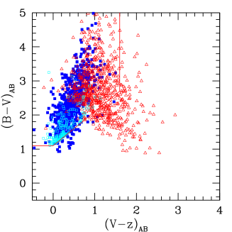
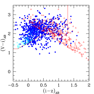
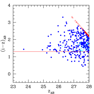
Figure 1: Color-color diagrams of $B$-, $V$- and $i$-dropouts for the std.f095.e03 model. (Blue) filled squares are galaxies with redshift in the specific interval of the selection, that is, [3.5-4.5], [4.5-5.5] and [5.5-6.5] for $B$-, $V$- and $i$-dropouts respectively. The open (cyan) squares represent the interlopers (see text for details), while the (red) open triangles are upper-limits in $B$,$V$ and $i$. For sake of clarity only the central galaxies (see Section 2.1) are here considered, (satellite galaxies have very similar colors).

The prediction of galaxy apparent magnitudes critically depends on dust attenuation, for which several uncertain parameters must be specified in grasil. Among all the parameters, we identify two of them as the crucial ones, namely $f_{\rm mol}$, the fraction of gas in molecular clouds, and $t_{\rm esc}$, the time after which OB stars get out of the highly obscured molecular cloud. In Fontanot et al. (2007) values of $f_{\rm mol}=0.5$ (typical of the Milky Way) and $t_{\rm esc}=10$ Myr were used to make predictions in the $K$ and sub-mm bands. However, when applied to our (much more dust-sensitive) Lyman-break candidates they give dust attenuations of more than 2 mag, definitely larger, e.g., than the values of 1.4, 1.15 and 0.8 mag assumed by Bouwens et al. (2007) for $B$-, $V$- and $i$-dropouts. Such parameter values may not be suitable for compact, gas-rich starbursting galaxies as our Lyman-break candidates are. In fact, higher molecular fractions are observed in galaxies where the ISM is more pressurized (see, e.g., Blitz & Rosolowsky, 2004); this would imply much lower attenuation by diffuse dust in the ISM (cirrus component).

We then run grasil using all combinations of $f_{\rm mol}=0.5$, 0.90, 0.95, 1.0 and $t_{\rm esc}=10$, 3, 1 Myr. Table 1 gives a list of all the runs performed. We use the model described in Section 2.1 with quasar-triggered galaxy winds (std), but perform also a few runs without winds (nowind) to check the effect of this (very uncertain) ingredient of the model. For sake of completeness we also show results for the same model (old) presented in Monaco et al. (2007) and Fontanot et al. (2007), with grasil run with a Salpeter IMF, but with $f_{\rm mol}=0.50$ and $t_{\rm esc}=3$ Myr, a combination which gives a best-fit of the Lyman-break luminosity functions.

For one of the models (std.f095.e03) we perform two runs with the addition of the Lyman-$\alpha$ emission line, either assuming a redshift-dependent $EW$ (std.f095.e03.lya1) or assuming a constant $EW$ (std.f095.e03.lya2), as motivated in Section 2.4

Figure 2: Selection function for $B$-, $V$- and $i$-dropouts for the std.f095.e03 model. The fraction of selected galaxies is computed in bins of redshift and apparent magnitude, and is reported as a tone of gray, as indicated in the right of each panel.

name	$f_{\rm mol}$	$t_{\rm esc}$	morgana run
		(Myr)
std.f050.e10	0.50	10	with quasar winds
std.f090.e10	0.90	10	”
std.f095.e10	0.95	10	”
std.f100.e10	1.00	10	”
std.f050.e03	0.50	3	”
std.f090.e03	0.90	3	”
std.f095.e03	0.95	3	”
std.f100.e03	1.00	3	”
std.f050.e01	0.50	1	”
std.f090.e01	0.90	1	”
std.f095.e01	0.95	1	”
std.f100.e01	1.00	1	”
std.f095.e03.lya1	0.95	3	with Ly$\alpha$ in emission
std.f095.e03.lya2	0.95	3	”
nowind.f090.e03	0.90	3	without quasar winds
nowind.f090.e01	0.90	1	”
nowind.f095.e03	0.95	3	”
old.f050.e03	0.50	3	2007 model

Table 1: Runs performed for this paper, with values of grasil parameters (see Section 2.3 for a brief description of the parameters) and indication of the morgana model used.

4 Results

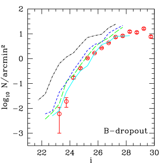
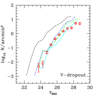
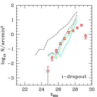
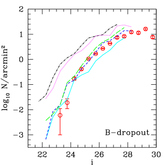
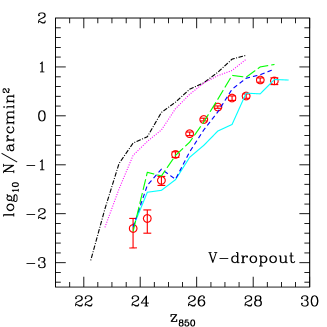
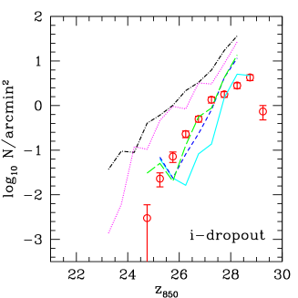
Figure 3: Number counts of $B$-, $V$- and $i$-dropouts. (Red) points are from Bouwens et al. (2007). Upper panels: models with $f_{\rm mol}=0.95$, std.f095.e10 (cyan solid lines), std.f095.e03 (green long-dashed lines) and std.f095.e01 (blue dashed lines) compared to the model without dust attenuation (black dot-dashed lines). Lower panels: models with $t_{\rm esc}=0.3$, std.f050.e03 (cyan solid lines), std.f090.e03 (blue dashed lines) and std.f095.e03 (green long-dashed lines) and std.f100.e03 (magenta dotted lines) also compared to the model without dust attenuation (black dot-dashed lines).

Figure 1 shows the color-color plots for the selection of the model $B$-, $V$- and $i$-dropouts, according to the criteria defined above. Here and in the next figure we use the std.f095.e03 model; here for sake of clarity only central galaxies with $z_{850}<28$, the resolution limit of the model, are used (satellite galaxies have very similar colors). All galaxies in the redshift intervals of the selection [3.5-4.5], [4.5-5.5] and [5.5-6.5] for $B$-,$V$- and $i$-dropouts respectively, are shown as full blue squares, or red triangles if they are upper limits. These are the same redshift intervals identified by Bouwens et al. (2007) as typical of Lyman-break galaxies at mean redshift of $z\sim 4$, $z\sim 5$ and $z\sim 6$. The few interlopers falling in the selection areas are marked as cyan open squares. For interlopers we mean galaxies with redshift in the interval [3.0-3.4] for the $B$-dropouts, [4.0-4.4] for the $V$-dropouts and [5.0-5.4] for the $i$-dropouts. Clearly, most galaxies in the relevant redshift interval are selected. Those that scatter out of the selection region are mostly faint galaxies with upper limits in the band from which they drop out; their colors are made less red by the upper limits. Figure 2 shows the selection function as a function of redshift and $i$ ($B$-dropouts) or $z_{850}$ ($V$- and $i$-dropouts) magnitude. Selected galaxies clearly tend to reside in the expected redshift range, though some $B$- and $V$-dropouts are lost at magnitudes fainter than $\sim 26$.

We first compare model predictions of $B$-, $V$- and $i$-dropouts with observed number counts, which are the directly observable quantity when complete spectroscopic samples are not available.

Figure  3 shows the effect of changing the grasil parameters $t_{\rm esc}$ and $f_{\rm mol}$ compared to the standard model without dust attenuation (black dot-dashed lines). We consider both the effect of changing $t_{\rm esc}$ keeping fixed the value of $f_{\rm mol}$ (upper panel), and the effect of varying $f_{\rm mol}$ at fixed $t_{\rm esc}$ (bottom panel). Model predictions for unabsorbed spectra drop at a magnitude $\sim 27.5$ (fainter for the $i$-dropouts). This is the typical magnitude of the central galaxy contained in the smallest resolved dark matter halo ($1.42\cdot 10^{10}$ M_⊙), fainter galaxies would be hosted in smaller, unresolved halos and are thus under-represented. It is worth noting that HUDF data are deeper than this limit Clearly this limit magnitude increases when dust attenuation is considered. When compared to Bouwens et al.’s observations (open red points in the Figure), number counts in absence of dust attenuation clearly overshoot the data (by about 2 mag). This shows how a correct modeling of attenuation is fundamental to best-fit the data. This feature clearly limits the predictive power of the model, because small variations of dust parameters within the allowed range give very large differences in the results.

The figure shows that the two parameters are degenerate; we identify the two combinations $(t_{\rm esc},f_{\rm mol})=(3\ {\rm Myr},0.95)$ (model std.f095.e03) and $(1\ {\rm Myr},0.90)$ (model std.f090.e01) as the best-fitting ones. This degeneration concerns the extinction, we in fact, expect to find differences in the IR due to the different distributions of temperature and optical depth of the two phases. The attenuations given by these best-fit models are roughly similar to the ones used by Bouwens et al. (1.4, 1.15 and 0.8 mag for $B$-, $V$- and $i$-dropouts) but are systematically higher for brighter galaxies. This is in line with the findings of Shapley et al. (2001): these authors reported for a large sample of Lyman-break galaxies at $z\sim 3$ an average $E(B-V)$ attenuation of 0.15 that correlates with magnitude, brighter objects being more absorbed. Expressed in terms of the same $E(B-V)$ quantity, our attenuation is $~{}0.1$ at the bright end and declines to $\sim 0.05$ for the faint objects.

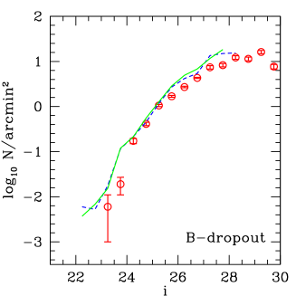
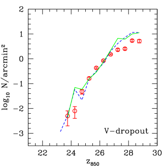
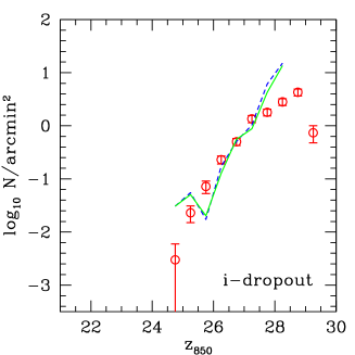
Figure 4: Number counts of $B$-, $V$- and $i$-dropouts. (Red) points are from Bouwens et al. (2007), the (blue) dashed and (green) solid lines give the predictions of the two best-fit models, respectively std.f090.e01 and std.f095.e03.

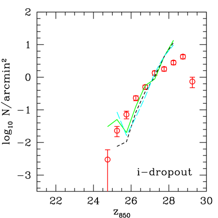
Figure 5: Number counts of $i$-dropouts. (Red) points are from Bouwens et al. (2007), the (green) solid line gives the predictions of the best-fit model std.f095.e03, the (black) dashed and the (cyan) long-dashed lines correspond to the same combination of parameters but with the contribution of Ly$\alpha$ emission line in the two different prescription discussed in Section 2.4 (black: std.f095.e03.lya1, cyan: std.f095.e03.lya2).

Figure 4 shows number counts for the two best-fit models. As expected, while the bright end is well reproduced with its redshift evolution (with a modest excess for the $B$-dropouts and possibly a dearth of bright $i$-dropouts), a clear excess of faint objects is present at $z_{850}\ga 27$, especially for the $V$-dropouts.

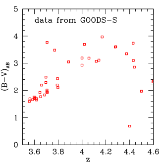
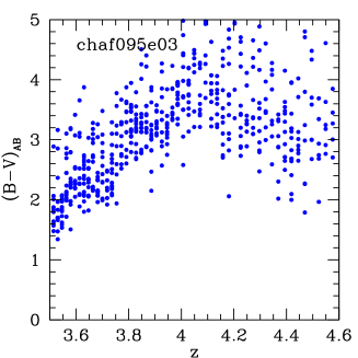
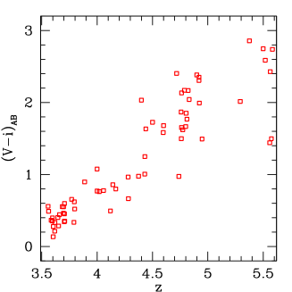
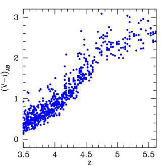
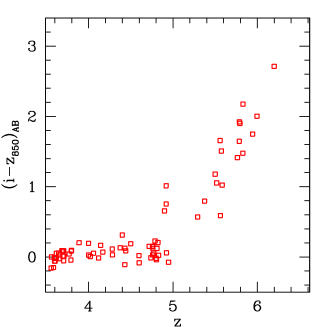
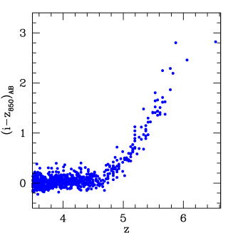
Figure 6: $B$-$V$, $V$-$i$ and $i$-$z_{850}$ colors of galaxies with $z_{850}<26.2$ as a function of redshift. Left panels: GOODS-S galaxies with spectroscopic redshift. Mid panels: GOODS-MUSIC galaxies with photometric redshifts. Black arrows indicate that the magnitude estimation is based on an upper limit at 1-$\sigma$. Right panels: model galaxies (std.f095.e03).

The inclusion of the Lyman-$\alpha$ line does not change much the predicted number counts of Lyman-break galaxies, with the exceptions of the $i$-dropouts, which are especially sensitive to the line. Figure 5 shows the effect of including the Lyman-$\alpha$ line, as explained in Section 2.4, to the std.f095.e03 best-fit model. As expected, the effect of the Lyman-$\alpha$ emission line is to make the $i$-$z_{850}$ color bluer, thus shifting the entrance in the selection criterion to slightly higher redshift and decreasing the number counts. This decrease is significant at the bright end, which is then underestimated by the model (in one case it also removes the kink at bright luminosity, which is due to the presence of few, high-weight galaxies - see Section 3), while the faint end is not strongly influenced. This conclusion does not change much with the choice of the $EW$. The inclusion of the Lyman-$\alpha$ emission line performed here is clearly tentative, but this test shows that our results are robust with respect to the inclusion of Lyman-$\alpha$ emission line under reasonable assumptions.

We then concentrate on the std.f095.e03 model, to understand to what extent model Lyman-break galaxies resemble the real ones.

Figure 6 shows the $B$-$V$, $V$-$i$ and $i$-$z_{850}$ colours of model and real galaxies as a function of redshift. Observed galaxies are shown both from the GOODS-S catalogue, with spectroscopic redshift, and for the GOODS-MUSIC catalogue, with photometric redshift, which clearly has many more galaxies. Only the galaxies brighter than $z_{850}<26.2$ are here considered, because of the 90 per cent completeness limit of the GOODS-MUSIC catalogue. As already noticed in Fig. 1, model galaxies present colours that closely resemble the observed ones, though they tend to be slightly redder, especially in $B$-$V$ at z$\sim$4 (at least compared to GOODS-MUSIC). Analogous conclusions can be drawn by considering the other best-fit model, std.f090.e01. This means that colours cannot be used to constrain the parameters. This conclusion is strenghtened by noting that the strong reddening of all colors with redshift is driven by IGM absorption.

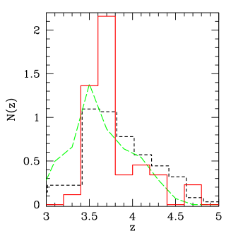
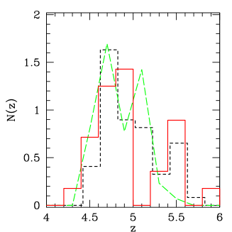
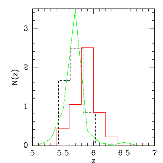
Figure 7: Redshift distribution for $B$-, $V$- and $i$-dropouts in the GOODS-S (red solid lines) and GOODS-MUSIC (black dashed lines) data samples ($z_{850}<26.2$) and in the std.f095.e03 model (green long-dashed lines).

Figure 7 shows the redshift distributions of model Lyman-break galaxies. We compare these predictions with the spectroscopic redshift distribution of GOODS-S galaxies (red solid lines) which constitute an incomplete sample (see Vanzella et al., 2008, 2009, for details) and with the photometric redshift distributions of GOODS-MUSIC (black dashed lines) and consider only galaxies brighter than $z_{850}=26.2$, the range where the GOODS-MUSIC sample is complete. The agreement is good though not perfect; this can be seen by comparing the average and standard deviation of the predicted redshift distributions, ($3.71\pm 0.35$; $4.88\pm 0.27$; $5.67\pm 0.22$; for $B$-,$V$- and $i$-dropout respectively), with those derived from Giavalisco et al. (2004), ($3.78\pm 0.34$; $4.92\pm 0.33$; $5.74\pm 0.36$; for the three candidates respectively), the GOODS-S spectroscopic sample ($3.78\pm 0.37$; $4.98\pm 0.39$; $5.92\pm 0.20$) and GOODS-MUSIC photometric sample ($3.81\pm 0.40$; $4.95\pm 0.37$; $5.74\pm 0.10$); however sample variance in the 150 arcmin² GOODS-S field is not negligible, so the level of agreement is considered satisfactory, especially if we consider that a confirmation of the validity of the redshift distribution is represented by the consistency between number counts and luminosity functions. Anyway, since the uncertainty related to the redshift measurements increases at higher redshifts where the detection is more difficult, this comparison should be taken with grain of salt. In particular, the number of available photometric redshifts of $i$-dropout galaxies is very low, because only few such galaxies are bright enough to be detected in $J$ and $K$ bands.

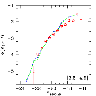
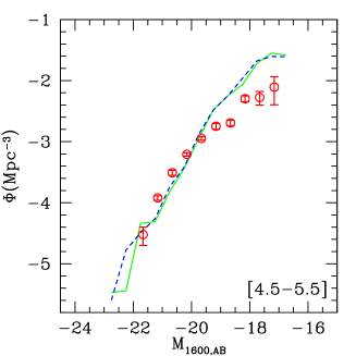
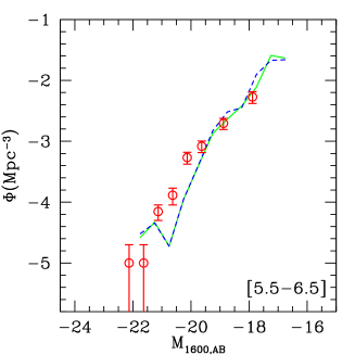
Figure 8: Luminosity function of $B$-, $V$- and $i$-dropouts. (Red) points are the estimate by Bouwens et al. (2007), (green) solid and (blue) dashed lines give predictions for the std.f095.e03 and std.f090.e01 models.

Bouwens et al. (2007) estimated the luminosity function of Lyman-break galaxies by scaling all observations to the HUDF ($5$-$\sigma$) depth of 29 in the $z_{850}$ band. Assuming that the $B$-dropout technique selects all star-forming (and not severely obscured) galaxies in the redshift interval $3.6<z<4.5$, they obtained selection functions of $V$- and $i$-dropouts by degrading images of low-$z$ $B$-dropout galaxies to reproduce observational biases at higher redshift, then estimating how many of them would be selected. As shown in figures 1 and 2, most model galaxies in that redshift range with high enough $z_{850}$ flux are $B$-dropouts, so it is fair to compare Bouwens et al.’s estimate to the luminosity function of all model galaxies in the redshift range $3.5<z<4.5$, $4.5<z<5.5$ and $5.5<z<6.5$. Figure 8 shows the luminosity function of the two best-fit models, compared to the Bouwens et al. (2007) determination, adjusted to take into account the slightly different cosmology. The agreement is again good at high luminosities (with a possible underestimate of the $i$-dropout bright tail), while a clear excess is visible in the faint tail, especially in the $V$-dropouts. We stress that this result is different from the one of figure 4 relative to number counts, because the two comparisons follow two different approaches: in the first case the model tries to reproduce exactly the observed quantity, in the second case the observers try to reconstruct a quantity more directly comparable with models, i.e. the luminosity function. The good agreement of data and model in terms of both number counts and luminosity functions cofirms that model galaxies closely resemble the observed population and their selection function. Moreover, the model follows very well the positive evolution (with time) of the knee of the luminosity functions, and this allows us to support Bouwens et al.’ conclusion that we are indeed witnessing the hierarchical build-up of the population of young galaxies.

Summing up, the morgana model reproduces the main observational properties (number counts, colours, selection functions, redshift distributions and estimated luminosity functions) of bright Lyman-break star-forming galaxies at $z>3.5$, (though a possible underestimate of the number of bright $i$-dropouts may be present); fainter galaxies, with $z_{850}\ga 27$, have acceptable properties but are over-produced. However, dust attenuation heavily depends on uncertain parameters of the ISM like $t_{\rm esc}$ and $f_{\rm mol}$, so that multiple solutions are equally acceptable.

5 A population of excess galaxies

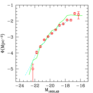
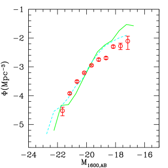
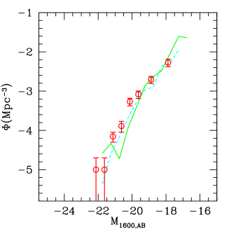
Figure 9: Luminosity function of $B$-, $V$- and $i$-dropouts. (Red) points are the estimate by Bouwens et al. (2007), (green) solid and (cyan) dashed lines give predictions for the nowind.f095.e03 and old.f050.e03 models.

Degeneracies in model predictions do not allow us to draw strong conclusions from the good agreement shown above between model and real Lyman-break galaxies at the bright end of the luminosity function. Indeed, parameter degeneracy is not due only to grasil; two morgana parameters, namely $n_{\rm dyn}$ and $n_{\rm quench}$ (see section 2.2) influence the star-formation rate density at $z>3$ but give small difference at lower redshift, where more constraints are available. To strengthen this point, we show in Figure 9 the prediction for the luminosity function of a model run without quasar-triggered galaxy winds (nowind.f095.e03) and the old.f090.e03 used in Fontanot et al. (2007), where a Salpeter IMF is used in place of Chabrier, and a slightly different cosmology with $\sigma_{8}=0.9$ is adopted. The last model is run on a $512^{3}$ box with slightly worse mass resolution. The fit is very similar to our best fits in all cases, and this confirms that bright Lyman-break galaxies cannot give strong constraints to models as long as dust attenuation is so uncertain. The reason why quasar winds do not affect this observable is the following. In our implemented scheme for quasar-triggered winds (Fontanot et al., 2006) radiation from an accreting black hole can evaporate some cold gas in the star-forming bulge; if the putative evaporation rate is higher than the star formation rate, then all the cold mass in the host bulge is removed. Quasar winds are then able to quench star formation in bulges (mergers), and this could lead to a suppression of star formation. However, due to the (modeled) delay between star formation and black-hole accretion, quasar winds take place when the star formation episode that has triggered accretion is almost over. The independence of the Lyman-break luminosity function on winds is a further demonstration of this.

Previous papers (Fontana et al., 2006; Cirasuolo et al., 2008; Marchesini et al., 2008; Fontanot et al., 2009) have shown that morgana presents a deficit of massive galaxies at $z>3$, when compared to the stellar mass function or to the K-band luminosity function. At the same time, morgana is able to reproduce the sub-mm counts of $z\sim 2$ starburst galaxies (Fontanot et al., 2007), and even shows a modest excess of bright $B$-dropouts (fig. 4). The two evidences of low stellar masses and a correctly high SFR are not contradictory: compared with similar models, morgana produces stronger cooling flows and then stronger bursts of star formation that are readily quenched by stellar feedback, so that the high levels of star formation are maintained for short times and do not produce higher amounts of stellar mass. Moreover, the apparent underestimate of stellar masses by morgana may be at least in part due to systematics in stellar mass estimates. Tonini et al. (2008) showed that inclusion of TP-AGBs in the Simple Stellar Population libraries give a significant downward revision of stellar masses at high redshifts or, equivalently, a boost to the $K$-band magnitude of model galaxies. According to Marchesini et al. (2008), our stellar mass function at $z\sim 3$ remains low at the $\sim 2\sigma$ level, but when we compare stellar masses of our model Lyman-break galaxies with estimates of Stark et al. (2009), which take into account TP-AGBs, we find a slight over-prediction, in contrast with the evidences mentioned above. It is then difficult at this stage to assess to what extent a good match of the bright end of the luminosity function of Lyman-break galaxies at $z\sim 4-5$ is in contrast with the apparent underestimate of the high end of the stellar mass function at $z\sim 3$.

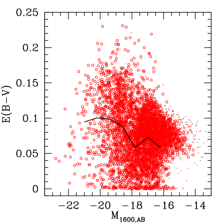
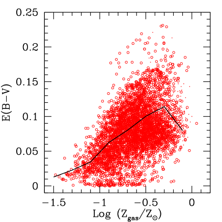
Figure 10: $E(B-V)$ attenuation as a function of the UV rest-frame luminosity $M_{1600,AB}$ (left panel) and gas-metallicity (referred to solar metallicity)(right panel). All model $V$-dropout galaxies at redshift about $5$ and with $Log(M_{\star})>7.75$, are here considered. Open circles refer to central galaxies. The black solid lines represent the ‘weighted’ mean values of $E(B-V)$ computed, respectively, for each bin of magnitude and gas-metallicity. $B$- and $i$-dropouts show a similar trend.

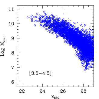
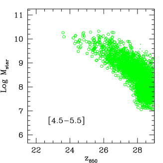
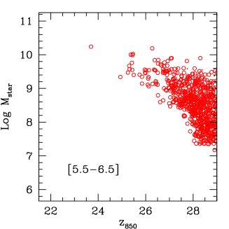
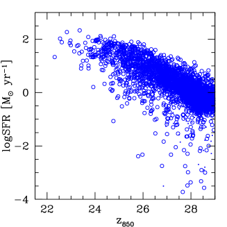
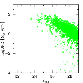
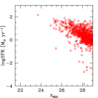
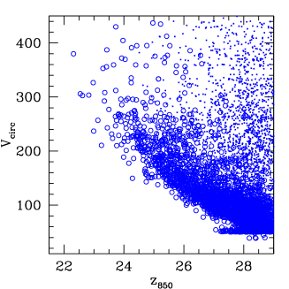
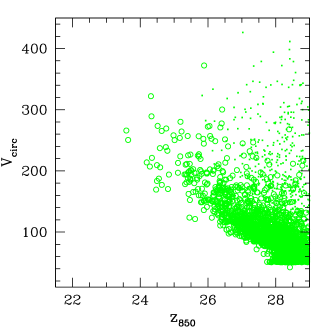
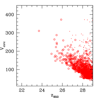
Figure 11: Properties of model Lyman-break galaxies as a function of $z_{850}$ magnitude, for the model std.f095.e03. Upper panels give stellar masses, mid panel give star formation rates, lower panels give dark matter halo circular velocities. Bigger open points refer to central galaxies.

Once the bright tail is matched, the model shows a clear excess of faint dropouts. Is this excess robust? From the one hand, as explained in the Introduction, the excess is expected: Fontanot et al. (2009) demonstrated that galaxies with stellar masses (at $z=0$) in the $10^{9}-10^{10}$ M_⊙ range are formed too early and are too passive since $z\sim 3$, and this is the main cause of the lack of (stellar mass and archaeological) downsizing in models. It follows that an excess of small star-forming galaxies must be present at higher redshift, and because the data go deeper than the completeness limit of the model, this excess must be visible. On the other hand, number counts at such deep magnitudes may well be incomplete. The use of the HUDF, and the careful analysis of Bouwens et al. to determine the selection functions, makes it unlikely that the model excess is purely due to sample incompleteness. Moreover, the reconstructed faint slope of the luminosity function is $\sim-1.7$, in agreement with many other determinations both at $z\geq 3$ (Yoshida et al., 2006; Beckwith et al., 2006; Oesch et al., 2007) and at $z\sim 2$ (Reddy & Steidel, 2008), while the slope of model luminosity functions is significantly steeper, in excess of $-2.0$.

Is this excess an artifact of dust extinction? in other words, is it possible that morgana is underestimating the star formation rate of bright galaxies (as well as stellar masses) but our ad-hoc tuning of dust parameters absorbs this discrepancy, creating an excess of faint galaxies? Figure 10 shows the $E(B-V)$ attenuation as a function of UV rest-frame luminosity $M_{1600,AB}$ (left panel) and gas-metallicity (right panel) for model $V$-dropout galaxies at $z\sim 5$ and with $Log(M_{\star})>7.75$; central galaxies are highlighted as empty circles. The solid black lines represent the ‘weighted’ mean values of $E(B-V)$ computed, respectively, for each bin of magnitude and gas-metallicity. For $B$- and $i$-dropouts we obtain a similar trend. The figure shows that the attenuation we obtain is only slightly lower ($E(B-V)\sim 0.1$ in place of 0.15) than what found by Shapley et al. (2001) at lower redshift, (but we are not using the same SED template of those authors because every galaxy in our model has its own SED), while, as mentioned above, the attenuation in the observed $i$ and $z_{850}$ bands is very similar to that used by Bouwens et al. (2007); the excess remains if we attenuate our galaxies as suggested in that paper. Moreover, the faint-end slope of model luminosity functions, in excess of $-2.0$, is inconsistent with the latest and very stable $-1.7$ value; with such a difference, an excess of faint galaxies will be obtained even if the bright tail is underestimated. This steep slope is in part due to to the fact that faint galaxies are less absorbed than bright ones, something that is well known in literature (see, e.g., Sanders & Mirabel, 1996), and is consistent with the trend found by Shapley et al. (2001) at $z\sim 3$. We conclude that it is unlikely that this excess is due to a peculiar behaviour of dust attenuation as predicted by grasil.

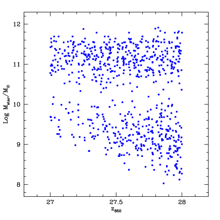
Figure 12: Stellar masses of the $z=0$ descendant galaxies of $V$-dropouts with $27<z_{850}<28$.

Other theoretical groups have compared their predictions of Lyman-break galaxies to data (see the reference list in the Introduction), but no group has clearly claimed to find a similar excess, with the exception of Poli et al. (2001, 2003), who compared the predictions of a semi-analytical model (Menci et al., 2002) with the reconstructed luminosity function of $I$ and $K$-selected samples (not color selected). They reported an excess of faint $I\sim 27$ galaxies at lower redshift, $z\sim 3$, which is even stronger than the one we find here. Also, Night et al. (2006) and Finlator et al. (2006), extracting catalogues of Lyman-break galaxies from N-body simulations, find rather steep luminosity functions, with slopes $\sim-2$. Night et al. (2006) discuss in some detail the implications of this steep slope, but claim broad consistency with available data; compared to the more recent determination of Bouwens et al., such steep slopes are nominally ruled out. There are two reasons why many groups may have not noticed such an excess: first, very deep fields like GOODS and the HUDF are required to reliably sample the $z_{850}\sim 27-28$ magnitude range, and these have been made available only recently. Second, a simple (and over-simplistic) magnitude-independent attenuation makes the excess less visible, so a more advanced tool as grasil is needed to notice it.

In the following of this section we try to assess whether the excess can be fixed simply by a better fine-tuning of model parameters, without spoiling the good match with local galaxies. To answer this question, we focus on the properties of the excess population. Figure 11 shows stellar masses, star formation rates and dark matter circular velocities of $B$-, $V$- and $i$-dropout galaxies as a function of apparent $z_{850}$ magnitude, for the best-fit model std.f095.e03; central galaxies are highlighted as empty circles. Excess galaxies with $z_{850}\sim 27-28$ are characterized by star formation rates of order of $\la 10$ M_⊙ yr^-1, stellar masses growing from $10^{8}-10^{9}$ M_⊙ at $z\sim 6$ to a factor of $\sim 3$ higher at $z\sim 4$, and the central ones are hosted in dark matter halos with masses in the range from $10^{11}$ to $10^{12}$ M_⊙, whose circular velocities are in excess of 100 km s^-1. Figure 12 shows the stellar mass of the $z=0$ descendant galaxies of $V$-dropouts with $27<z_{85}<28$. Roughly half of them do not grow much in mass since $z\sim 5$, thus falling in the stellar mass range of galaxies that are too old in models. The other half merge with larger galaxies to end up at the knee of the stellar mass function. In many papers, like e.g. Santini & et al. (2008), the observed specific star formation rates of massive galaxies is found to be higher than model predictions by a factor at least of $\sim 4$, which is apparently at variance with the good match of the growth of stellar mass in the same galaxies since $z\sim 3$ (Fontana et al., 2006). The puzzle may be solved if the excess population of small galaxies contributes to inflate the growth of massive galaxies by minor mergers, thus compensating for the lower star formation rates. We propose this as a plausible explanation, although more stable estimates of star formation rates in galaxies are necessary to assess this problem.

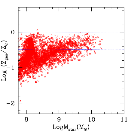
Figure 13: Stellar mass – gas metallicity relation for model galaxies at $z=5$. In this plot all galaxies in the box are used. Bigger open points refer to central galaxies. The two horizontal lines mark solar and $1/3$ solar metallicities. We removed galaxies with less than 10 per cent gas fraction.

An important hint on the mechanism responsible for the excess of faint galaxies comes from their metallicities $Z$. Observations show that metallicities measured from emission lines decline with redshift, and this decline is stronger for smaller galaxies. This has been measured at $z\sim 2$ by Savaglio et al. (2005) and by Erb et al. (2006), Erb (2007), and at $z\sim 3$ by Maiolino et al. (2008), but some measures exist at higher redshift (Ando et al., 2007) that seem to confirm the trend up to $z\sim 6$. Besides, Pettini et al. (2001) report a value of $1/3$ solar as the typical metallicity of $z\sim 3$ Lyman-break galaxies. We show in figure 13 the predicted metallicities of the gas component of galaxies at $z=5$ as a function of their galaxy stellar mass. We show gas metallicities because these are measured from emission lines. A mass-metal relation is visible, but with a very high normalization, for which $10^{10}$ M_⊙ galaxies are already enriched above $1/3$ solar, the typical gas metallicity of $z\sim 3$ Lyman-break galaxies. Moreover, a blob of small, highly enriched galaxies is visible, that is probably absent in the real world. These high metallicities justify the slightly redder colours of model galaxies and the shift toward lower redshift of the selection function, and may be at the origin of the underestimate of the number of bright $i$-dropouts. High metallicities at high redshift are a common problem of galaxy formation models, as pointed out in Maiolino et al. (2008); relatively high metallicities at $z\sim 2-3$ are reported by Guo & White (2008), and studying model predictions for the Milky Way De Lucia & Helmi (2008) noticed a dearth of low metallicity halo stars, due to excessive enrichment of small galaxies (before they become Milky Way satellite) at high redshift. Can this mismatch in gas metallicity create the excess of faint galaxies? Observations (Maiolino et al., 2008) suggest a downsizing trend for metal enrichment, with the stellar mass-gas metallicity relation steepening at high redshift. Our relation is rather flat, so that we are probably overestimating gas metallicity more in fainter objects. If more metals give higher attenuation, this mismatch would lead to an artificial flattening of the LF, thus decreasing the excess of faint Lyman-break galaxies rather than creating it.

There is a broad consensus among modelers on the fact that AGN feedback is most effective in massive galaxies at low redshift, so the excess galaxies should be suppressed by stellar feedback. This should work in the direction of creating strong gas and metal outflows, so as to keep low both stellar mass and metallicity. Coming back to the question on whether this excess can be suppressed by fine-tuning model parameters, it is easy to do it by increasing the efficiency of stellar feedback, but at the cost of destroying the good fit of the stellar mass function at low redshift. Indeed, as clear in Figure 11, such galaxies, though small, are hosted in relatively large dark matter halos with circular velocities well in excess of 100 km s^-1. Because the efficiency of gas removal mainly scales with halo circular velocity (as found since the seminal work of Dekel & Silk, 1986), this would be done at the cost of suppressing also star formation in those $10^{12}$ M_⊙ halos at $z=0$ in which star formation efficiency is highest, thus destroying the good agreement with the local stellar mass function (and luminosity functions as well).

Stellar feedback is manily driven by SNe, and each SN produces roughly $10^{51}$ erg of energy, which translates into $10^{49}$ erg per M_⊙ of stars formed if roughly 1 SN explodes each 100 M_⊙ of solar masses. If a fraction $\varepsilon$ of SN energy is injected in the ISM instead of being quickly radiated away ($\varepsilon\sim 0.3$ in our model), the velocity $v_{\rm eject}$ at which a mass $M_{\rm eject}$ can be accelerated by a mass $M_{\star}$ of stars formed is $v_{\rm eject}\sim 500\sqrt{(\varepsilon/0.3)M_{\star}/M_{\rm eject}}$ km s^-1. As a result, one M_⊙ of stars can not eject much more than one M_⊙ of gas out of a halo with circular velocity of $\sim 200$ km $s^{-1}$ (and escape velocity higher by the canonical factor of $\sqrt{2}$). In order to limit the number and metal content of faint Lyman-break galaxies hosted in 100 km/s halos at $z\sim 5$, $v_{\rm eject}$ must be higher than it is at $z\sim 0$, and this can be obtained as follows: (i) increasing energy feedback efficiency $\varepsilon$ (if not the SN energy), (ii) increasing the number of SNe per solar mass of stars formed, (iii) decreasing halo circular velocities (or their number at fixed $V_{c}$). The first solution would imply that feedback works differently in such starburst, with the paradoxical conclusion that feedback can be most efficient in the densest environments. Anyway, the gain factor is unlikely to be very high, because if 32 per cent of SN energy (in discs) is available for feedback, as assumed in this paper, the gain cannot be higher than a factor of three in energy (or $v_{\rm eject}^{2}$). Things would change if such SNe were more energetic than their low-redshift and high-metallicity counterparts. Solution (ii) would be obtained by assuming a different, more top-heavy IMF in these galaxies, while solution (iii) would require that dark matter is not completely cold and collisionless as assumed.

In all cases, a solution of this discrepancy, and a proper reproduction of stellar mass and archaeological downsizing, requires some deep change in the models, be it a more sophisticated feedback scheme, more energetic SNe at high redshift, a varying IMF or a different dark matter theory. Moreover, this question is of great interest because, due to their steep luminosity function, such galaxies would contain most produced metals, so they are very important contributors to metal pollution of the IGM.

While theoretical progress can be achieved by exploring the ideas given above, observational breakthroughs will have to wait the next generation of telescopes. Indeed, while the photometric selection of Lyman-break galaxies is feasible with the current facilities up to magnitude $z_{850}\sim$28, even though on a relatively small field like GOODS, the spectroscopic observations of relevant features like the break of the continuum blueward the $Ly\alpha$ line and the detection of the ultraviolet absorption lines is still challenging for sources fainter than $z_{850}\sim 25.5$. Beyond this limit the main spectral feature is the Lyman $\alpha$ emission line (if present), often observed without continuum; only composite spectra allow to increase the signal-to-noise. Future observations in the next decade with ground-based 30-40m class telescopes (e.g. TMT, E-ELT), with ALMA and from the space with JWST will be crucial to make an observational breakthrough; one of the main goals of these facilities is to perform spectroscopic surveys of faint sources, reaching easily $z_{850}\sim 27$. Not only the precise estimation of the redshift will be possible, but the validation of the dropout technique at that level and information on the total mass (from the stellar velocity dispersion), mass distribution and rotation curve, metallicity, dust content, galactic wind energetics and stellar population distribution will be straightforward to derive from 30-40m spectra of the galaxies already discovered in the 8-10m surveys. The rich phenomenology revealed by these spectra will give us new insight on the formation of galaxies, that will complement the theoretical efforts made in the next years.

6 Summary

We have compared the predictions of morgana$+$grasil (Monaco et al., 2007; Silva et al., 1998; Fontanot et al., 2007) with data of Lyman-break galaxies at $z\sim 4-6$. Model predictions have been produced by simulating deep ACS-HST fields, taking into account photometric errors as in the GOODS-S survey (Giavalisco et al., 2004), and the effect of Lyman-alpha emission line. They have been compared to number counts of $B$- $V$- and $i$-dropouts, scaled to the HUDF sensitivity by Bouwens et al. (2007), colour evolution, redshift distributions and selection function of GOODS-S (Vanzella et al., 2009) and GOODS-MUSIC (Grazian et al., 2006) galaxies, and luminosity functions estimated by Bouwens et al. (2007).

Model galaxies closely resemble the observed ones in terms of sizes, stellar masses, colors, dark matter halo properties and spatial distribution but have significantly higher metallicities. However for such galaxies, observed at rest-frame UV wavelengths, dust attenuation is as important as uncertain. We find that reasonable tuning of grasil parameters, namely escape time $t_{\rm esc}$ of stars from the parent molecular cloud and fraction $f_{\rm mol}$ of gas in the molecular phase, can result in more than a magnitude difference. The two parameters are also degenerate, i.e. decreasing the first has a similar effect as increasing the second and vice versa. These parameters are also degenerate with model parameters that regulate the amount of star formation in high-redshift halos.

Fixing the parameters it is possible to reproduce the bright end of the number counts and luminosity functions, with a modest overestimate of the number of bright $B$-dropouts and a possible underestimate of bright $i$-dropouts. We then notice an excess of faint ($z_{850}\ga 27$) star-forming galaxies, especially when considering $V$-dropouts at $4.5<z<5.5$. This excess is unlikely to be due to sample incompleteness or to some peculiar behaviour of grasil dust attenuation. Fontanot et al. (2009), found a serious discrepancy between models of galaxy formation (including morgana) and data for galaxies in the mass range $10^{9}-10^{10.5}$ M_⊙ at $z=0$. These form too early in the models, are too passive at $z<3$ and host too old stellar populations at low redshift. This clearly implies an excess of small star-forming galaxies at high redshift that forces modelers to suppress star formation at later time, so as to recover the correct number of small galaxies at $z=0$.

We define a class of galaxies which are over-produced by the model. These faint Lyman-break galaxies, forming stars at $\la 10$ M_⊙ yr^-1, have masses that grow in stellar mass from $z\sim 6$, where their mass is $\sim 3\times 10^{8}-3\times 10^{9}$ M_⊙, to $z\sim 4$, where their mass has grown to $\sim 10^{9}-10^{10}$ M_⊙. They are hosted in relatively massive dark matter halos, with masses in the range $10^{11}-10^{12}$ M_⊙ and circular velocities in excess of 100 km s^-1. These galaxies show a stellar mass – gas metallicity relation which is too high compared to the (sparse) available evidence. At $z=0$ roughly half of them are found in small galaxies, the other half having evolved into more massive objects.

We conclude that some feedback mechanism should be at play, causing star formation in these galaxies to be suppressed by strong gas and metal outflows. These metals would then be important polluters of the IGM, and because this pollution takes place before the peak of cosmic star formation, constraining this process is of great importance also for IGM studies. As originally shown by Dekel & Silk (1986), the amount of ejected mass mainly scales with the halo circular velocities, and this is true for most semi-analytic galaxy formation models. In this way, under very simple assumptions, a suppression of these galaxies implies a suppression of star formation in those $10^{12}$ M_⊙ halos for which the peak of efficiency of star formation is expected at $z=0$. Solving this discrepancy requires either some form of feedback that, surprisingly, is most effective at the highest gas densities, or some more exotic solution, like higher SN energy in dense environments with low metallicity, a top-heavy IMF or a not perfectly cold and collisionless dark matter which suppresses such compact halos. Observational breakthroughs able to clarify the phisical processes responsible for the suppression of these “excess” galaxies may be obtained with the future 30-40m optical telescopes, ALMA and JWST; a strong theoretical and numerical effort on this topic should be carried out in the next future to produce predictions that can be tested by future observations.

References

- Ando et al. (2007) Ando M., Ohta K., Iwata I., Akiyama M., Aoki K., Tamura N., 2007, PASJ, 59, 717
- Baugh (2006) Baugh C. M., 2006, Reports of Progress in Physics, 69, 3101
- Baugh et al. (2005) Baugh C. M., Lacey C. G., Frenk C. S., Granato G. L., Silva L., Bressan A., Benson A. J., Cole S., 2005, MNRAS, 356, 1191
- Beckwith et al. (2006) Beckwith S. V. W., Stiavelli M., Koekemoer A. M., Caldwell J. A. R., Ferguson H. C., Hook R., Lucas R. A., Bergeron L. E., Corbin M., Jogee S., Panagia N., Robberto M., Royle P., Somerville R. S., Sosey M., 2006, AJ, 132, 1729
- Blaizot et al. (2004) Blaizot J., Guiderdoni B., Devriendt J. E. G., Bouchet F. R., Hatton S. J., Stoehr F., 2004, MNRAS, 352, 571
- Blitz & Rosolowsky (2004) Blitz L., Rosolowsky E., 2004, ApJ, 612, L29
- Bouwens et al. (2007) Bouwens R. J., Illingworth G. D., Franx M., Ford H., 2007, ApJ, 670, 928
- Chabrier (2003) Chabrier G., 2003, ApJ, 586, L133
- Cirasuolo et al. (2008) Cirasuolo M., McLure R. J., Dunlop J. S., Almaini O., Foucaud S., Simpson C., 2008, ArXiv e-prints, 804
- Conroy et al. (2007) Conroy C., Wechsler R. H., Kravtsov A. V., 2007, ApJ, 668, 826
- De Lucia & Helmi (2008) De Lucia G., Helmi A., 2008, MNRAS, 391, 14
- Dekel & Silk (1986) Dekel A., Silk J., 1986, ApJ, 303, 39
- Eisenstein & Hu (1998) Eisenstein D. J., Hu W., 1998, ApJ, 496, 605
- Erb (2007) Erb D. K., 2007, in Emsellem E., Wozniak H., Massacrier G., Gonzalez J.-F., Devriendt J., Champavert N., eds, EAS Publications Series Vol. 24 of EAS Publications Series, Galaxy Metallicities, Masses and Outflows at Redshifts 1Z3: An Observational Perspective. pp 191–202
- Erb et al. (2006) Erb D. K., Shapley A. E., Pettini M., Steidel C. C., Reddy N. A., Adelberger K. L., 2006, ApJ, 644, 813
- Finlator et al. (2006) Finlator K., Davé R., Papovich C., Hernquist L., 2006, ApJ, 639, 672
- Fontana et al. (2006) Fontana A., Salimbeni S., Grazian A., Giallongo E., Pentericci L., Nonino M., Fontanot F., Menci N., et al. 2006, A&A, 459, 745
- Fontanot et al. (2009) Fontanot F., De Lucia G., Monaco P., Somerville R. S., Santini P., 2009, ArXiv e-prints
- Fontanot et al. (2006) Fontanot F., Monaco P., Cristiani S., Tozzi P., 2006, MNRAS, 373, 1173
- Fontanot et al. (2007) Fontanot F., Monaco P., Silva L., Grazian A., 2007, MNRAS, 382, 903
- Fontanot et al. (2009) Fontanot F., Somerville R. S., Silva L., Monaco P., Skibba R., 2009, MNRAS, 392, 553
- Gao et al. (2008) Gao L., Navarro J. F., Cole S., Frenk C. S., White S. D. M., Springel V., Jenkins A., Neto A. F., 2008, MNRAS, 387, 536
- Giavalisco et al. (2004) Giavalisco M., Dickinson M., Ferguson H. C., Ravindranath S., Kretchmer C., Moustakas L. A., Madau P., Fall S. M., Gardner J. P., Livio M., Papovich C., Renzini A., Spinrad H., Stern D., Riess A., 2004, ApJ, 600, L103
- Grazian et al. (2006) Grazian A., Fontana A., de Santis C., Nonino M., Salimbeni S., Giallongo E., Cristiani S., Gallozzi S., Vanzella E., 2006, A&A, 449, 951
- Guo & White (2008) Guo Q., White S. D. M., 2008, ArXiv e-prints
- Harford & Gnedin (2003) Harford A. G., Gnedin N. Y., 2003, ApJ, 597, 74
- Kennicutt (1998) Kennicutt Jr. R. C., 1998, ApJ, 498, 541
- Kimm et al. (2008) Kimm T., Somerville R. S., Yi S. K., van den Bosch F. C., Salim S., Fontanot F., Monaco P., Mo H., Pasquali A., Rich R. M., Yang X., 2008, ArXiv e-prints
- Kitzbichler & White (2007) Kitzbichler M. G., White S. D. M., 2007, MNRAS, 376, 2
- Lee et al. (2008) Lee S.-K., Idzi R., Ferguson H. C., Somerville R. S., Wiklind T., Giavalisco M., 2008, ArXiv e-prints
- Madau (1995) Madau P., 1995, ApJ, 441, 18
- Maiolino et al. (2008) Maiolino R., Nagao T., Grazian A., Cocchia F., Marconi A., Mannucci F., Cimatti A., Pipino e. a., 2008, A&A, 488, 463
- Mao et al. (2007) Mao J., Lapi A., Granato G. L., de Zotti G., Danese L., 2007, ApJ, 667, 655
- Marchesini et al. (2008) Marchesini D., van Dokkum P. G., Forster Schreiber N. M., Franx M., Labbe’ I., Wuyts S., 2008, ArXiv e-prints
- Menci et al. (2002) Menci N., Cavaliere A., Fontana A., Giallongo E., Poli F., 2002, ApJ, 575, 18
- Monaco (2004) Monaco P., 2004, MNRAS, 352, 181
- Monaco & Fontanot (2005) Monaco P., Fontanot F., 2005, MNRAS, 359, 283
- Monaco et al. (2007) Monaco P., Fontanot F., Taffoni G., 2007, MNRAS, 375, 1189
- Monaco et al. (2006) Monaco P., Murante G., Borgani S., Fontanot F., 2006, ApJ, 652, L89
- Monaco et al. (2002) Monaco P., Theuns T., Taffoni G., 2002, MNRAS, 331, 587
- Monaco et al. (2002) Monaco P., Theuns T., Taffoni G., Governato F., Quinn T., Stadel J., 2002, ApJ, 564, 8
- Nagamine (2002) Nagamine K., 2002, ApJ, 564, 73
- Nagamine et al. (2008) Nagamine K., Ouchi M., Springel V., Hernquist L., 2008, ArXiv e-prints
- Nagamine et al. (2004) Nagamine K., Springel V., Hernquist L., Machacek M., 2004, MNRAS, 350, 385
- Night et al. (2006) Night C., Nagamine K., Springel V., Hernquist L., 2006, MNRAS, 366, 705
- Oesch et al. (2007) Oesch P. A., Stiavelli M., Carollo C. M., Bergeron L. E., Koekemoer A. M., Lucas R. A., Pavlovsky C. M., Trenti M., Lilly S. J., Beckwith S. V. W., Dahlen T., Ferguson H. C., Gardner J. P., Lacey C., Mobasher B., Panagia N., Rix H.-W., 2007, ApJ, 671, 1212
- Overzier et al. (2008) Overzier R., Guo Q., Kauffmann G., De Lucia G., Bouwens R., Lemson G., 2008, ArXiv e-prints
- Pettini et al. (2001) Pettini M., Shapley A. E., Steidel C. C., Cuby J.-G., Dickinson M., Moorwood A. F. M., Adelberger K. L., Giavalisco M., 2001, ApJ, 554, 981
- Poli et al. (2003) Poli F., Giallongo E., Fontana A., Menci N., Zamorani G., Nonino M., Saracco P., Vanzella E., Donnarumma I., Salimbeni S., Cimatti A., Cristiani S., Daddi E., D’Odorico S., Mignoli M., Pozzetti L., Renzini A., 2003, ApJ, 593, L1
- Poli et al. (2001) Poli F., Menci N., Giallongo E., Fontana A., Cristiani S., D’Odorico S., 2001, ApJ, 551, L45
- Reddy & Steidel (2008) Reddy N. A., Steidel C. C., 2008, ArXiv e-prints
- Sanders & Mirabel (1996) Sanders D. B., Mirabel I. F., 1996, ARA&A, 34, 749
- Santini & et al. (2008) Santini P., et al. 2008, submitted to A&A
- Savaglio et al. (2005) Savaglio S., Glazebrook K., Le Borgne D., Juneau S., Abraham R. G., Chen H.-W., Crampton D., McCarthy P. J., Carlberg R. G., Marzke R. O., Roth K., Jørgensen I., Murowinski R., 2005, ApJ, 635, 260
- Shapley et al. (2001) Shapley A. E., Steidel C. C., Adelberger K. L., Dickinson M., Giavalisco M., Pettini M., 2001, ApJ, 562, 95
- Shapley et al. (2003) Shapley A. E., Steidel C. C., Pettini M., Adelberger K. L., 2003, ApJ, 588, 65
- Silva et al. (1998) Silva L., Granato G. L., Bressan A., Danese L., 1998, ApJ, 509, 103
- Somerville et al. (2008) Somerville R. S., Hopkins P. F., Cox T. J., Robertson B. E., Hernquist L., 2008, MNRAS, 391, 481
- Somerville et al. (2001) Somerville R. S., Primack J. R., Faber S. M., 2001, MNRAS, 320, 504
- Spergel (2005) Spergel D. N., 2005, in Lidman C., Alloin D., eds, The Cool Universe: Observing Cosmic Dawn Vol. 344 of Astronomical Society of the Pacific Conference Series, The Cosmic Microwave Background as a Cosmological Probe. pp 29–+
- Stark et al. (2009) Stark D. P., Ellis R. S., Bunker A., Bundy K., Targett T., Benson A., Lacy M., 2009, ArXiv e-prints
- Taffoni et al. (2003) Taffoni G., Mayer L., Colpi M., Governato F., 2003, MNRAS, 341, 434
- Taffoni et al. (2002) Taffoni G., Monaco P., Theuns T., 2002, MNRAS, 333, 623
- Tonini et al. (2008) Tonini C., Maraston C., Devriendt J., Thomas D., Silk J., 2008, ArXiv e-prints
- Vanzella et al. (2008) Vanzella E., Cristiani S., Dickinson M., Giavalisco M., Kuntschner H., Haase J., Nonino M., Rosati P. e. a., 2008, A&A, 478, 83
- Vanzella et al. (2006) Vanzella E., Cristiani S., Dickinson M., Kuntschner H., Nonino M., Rettura A., Rosati P., Vernet R., et al. 2006, A&A, 454, 423
- Vanzella et al. (2009) Vanzella E., Giavalisco M., Dickinson M., Cristiani S., Nonino M., Kuntschner H., Popesso P., Rosati P., Renzini A., Stern D., Cesarsky C., Ferguson H. C., Fosbury R. A. E., the GOODS Team 2009, ArXiv e-prints
- Vega et al. (2005) Vega O., Silva L., Panuzzo P., Bressan A., Granato G. L., Chavez M., 2005, MNRAS, 364, 1286
- Verhamme et al. (2008) Verhamme A., Schaerer D., Atek H., Tapken C., 2008, A&A, 491, 89
- Viola et al. (2008) Viola M., Monaco P., Borgani S., Murante G., Tornatore L., 2008, MNRAS, 383, 777
- Wang et al. (2008) Wang J., De Lucia G., Kitzbichler M. G., White S. D. M., 2008, MNRAS, 384, 1301
- Weinberg et al. (2002) Weinberg D. H., Hernquist L., Katz N., 2002, ApJ, 571, 15
- Yoshida et al. (2006) Yoshida M., Shimasaku K., Kashikawa N., Ouchi M., Okamura S., Ajiki M., Akiyama M., et al. A., 2006, ApJ, 653, 988