Chemical Power for Microscopic Robots in Capillaries

Abstract

The power available to microscopic robots (nanorobots) that oxidize bloodstream glucose while aggregated in circumferential rings on capillary walls is evaluated with a numerical model using axial symmetry and time-averaged release of oxygen from passing red blood cells. Robots about one micron in size can produce up to several tens of picowatts, in steady-state, if they fully use oxygen reaching their surface from the blood plasma. Robots with pumps and tanks for onboard oxygen storage could collect oxygen to support burst power demands two to three orders of magnitude larger. We evaluate effects of oxygen depletion and local heating on surrounding tissue. These results give the power constraints when robots rely entirely on ambient available oxygen and identify aspects of the robot design significantly affecting available power. More generally, our numerical model provides an approach to evaluating robot design choices for nanomedicine treatments in and near capillaries.

Keywords: nanomedicine, nanorobotics, capillary, power, numerical model, oxygen transport

1 Introduction

Nanotechnology has the potential to revolutionize health care [65, 66, 49, 63]. A current example is enhanced imaging with nanoscale particles [86, 68]. Future possibilities include programmable machines comparable in size to cells [26, 27, 30, 59]. Such microscopic robots (“nanorobots”) could provide significant medical benefits [27, 65, 39].

Realizing these benefits requires fabricating the robots cheaply and in large numbers. Such fabrication is beyond current technology, but could result from ongoing progress in developing nanoscale devices. One approach is engineering biological systems, e.g., RNA-based logic inside cells [92] and bacteria attached to nanoparticles [60]. However, biological organisms have limited material properties and computational speed. Instead, we consider machines based on plausible extensions of currently demonstrated nanoscale electronics, sensors and motors [7, 12, 19, 20, 46, 31, 58, 64, 89] and relying on directed assembly [51]. These components enable nonbiological robots that are stronger, faster and more flexibly programmed than is possible with biological organisms.

A major challenge for nanorobots arises from the physics of their microenvironments, which differ in several significant respects from today’s larger robots. First, the robots will often operate in fluids containing many moving objects, such as cells, dominated by viscous forces. Second, thermal noise is a significant source of sensor error and Brownian motion limits the ability to follow precisely specified paths. Finally, power significantly constrains the robots [57, 77], especially for long-term applications where robots may passively monitor for specific rare conditions (e.g., injury or infection) and must respond rapidly when those conditions occur.

Individual robots moving passively with the circulation can approach within a few cell diameters of most tissue cells of the body. To enable passing through even the smallest vessels, the robots must be at most a few microns in diameter. This small size limits the capabilities of individual robots. For tasks requiring greater capabilities, robots could form aggregates by using self-assembly protocols [27]. For robots reaching tissues through the circulation, the simplest aggregates are formed on the inner wall of the vessel. Robots could also aggregate in tissue spaces outside small blood vessels by exiting capillaries via diapedesis [27], a process similar to that used by immune cells [2].

Aggregates of robots in one location for an extended period of time could be useful in a variety of tasks. For example, they could improve diagnosis by combining multiple measurements of chemicals [44]. Using these measurements, the aggregate could give precise temporal and spatial control of drug release [27, 30] as an extension of an in vitro demonstration using DNA computers [9]. Using chemical signals, the robots could affect behavior of nearby tissue cells. For such communication, molecules on the robot’s surface could mimic existing signalling molecules to bind to receptors on the cell surface [27, 29]. Examples include activating nerve cells [88] and initiating immune response [29], which could in turn amplify the actions of robots by recruiting cells to aid in the treatment. Such actions would be a small-scale analog of robots affecting self-organized behavior of groups of organisms [36]. Aggregates could also monitor processes that take place over long periods of time, such as electrical activity (e.g., from nearby nerve cells), thereby extending capabilities of devices tethered to nanowires introduced through the circulatory system [54]. In these cases, the robots will likely need to remain on station for tens of minutes to a few hours or even longer.

The aggregate itself could be part of the treatment by providing structural support, e.g., in rapid response to injured blood vessels [28]. Aggregates could perform precise microsurgery at the scale of individual cells, extending surgical capabilities of simpler nanoscale devices [52]. Since biological processes often involve activities at molecular, cell, tissue and organ levels, such microsurgery could complement conventional surgery at larger scales. For instance, a few millimeter-scale manipulators, built from micromachine (MEMS) technology, and a population of microscopic devices could act simultaneously at tissue and cellular size scales, e.g., for nerve repair [80, 45].

For medical tasks of limited duration, onboard fuel created during robot manufacture could suffice. Otherwise, the robots need energy drawn from their environment, such as converting externally generated vibrations to electricity [90] or chemical generators [27]. Power and a coarse level of control can be combined by using an external source, e.g., light, to activate chemicals in the fluid to power the machines in specific locations [83], similar to nanoparticle activation during photodynamic therapy [8], or by using localized thermal, acoustic or chemical demarcation [27].

This paper examines generating power for long-term robot activity from reacting glucose and oxygen, which are both available in the blood. Such a power source is analogous to bacteria-based fuel cells whose enzymes enable full oxidation of glucose [17, 55, 56]. We describe a computationally feasible model incorporating aspects of microenvironments with significant effect on robot performance but not previously considered in robot designs, e.g., kinetic time constants determining how rapidly chemical concentrations adjust to robot operations. As a specific scenario, we focus on modest numbers of robots aggregated in capillaries.

A second question we consider is how the robots affect surrounding tissue. Locally, the robots compete for oxygen with the tissue and also physically block diffusion out of the capillary. Robot power generation results in waste heat, which could locally heat the tissue. The robot oxygen consumption could also have longer range effects by depleting oxygen carried in passing red blood cells.

In the remainder of this paper, we present a model of the key physical properties relevant to power generation for robots using oxygen and glucose in the blood plasma. Using this model, we then evaluate the steady-state power generation capabilities of aggregated robots and how they influence surrounding tissue.

2 Modeling Physical Processes for Microscopic Robots

We consider microscopic robots using oxygen and glucose available in blood plasma as the robots’ power source. This scenario involves fluid flow, chemical diffusion, power generation from reacting chemicals and waste heat production. Except for the simplest geometries, behaviors must be computed numerically, e.g., via the finite element method [81]. Computational feasibility requires a choice between level of detail of modeling individual devices and the scale of the simulation, both in number of devices and physical size of the environment considered. For microscopic biological environments relevant for nanorobots, detailed physical properties may not be known or measurable with current technology, thereby limiting the level of detail possible to specify.

This section describes our model. The simplifying approximations are similar to those used in biophysical models of microscopic environments, such as oxygen transport in small blood vessels with diffusion into surrounding tissue [62, 67]. We focus on steady-state behavior indicating long-term robot performance when averaged over short-term changes in the local environment such as individual blood cells (exclusively erythrocytes, not white cells or platelets unless noted otherwise) passing the robots.

2.1 Blood Vessel and Robot Geometry

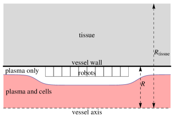
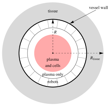
(a)	(b)

Figure 1: Schematic geometry of vessel, robots and surrounding tissue. The relative sizes of the regions are not to scale for the parameters of our model (described in Section 2.9). (a) A slice through the axially symmetric geometry with the vessel axis at the bottom, showing a cross section of 10 rings of robots. Fluid flows through the vessel from left to right, with varying speed depending on distance to the vessel wall. (b) Vessel cross section at the position of one ring of robots.

Evaluating behavior in general three-dimensional geometries is computationally intensive. Simplified physical models give useful insight with significantly reduced computational requirements [67]. Such simplifications include using two-dimensional and axially-symmetric three-dimensional geometries. The latter case, appropriate for behavior within vessels, has physical properties independent of angle of rotation around the vessel axis. We adopt this approach and consider the axially-symmetric geometry illustrated in Fig. 1: a segment of a small vessel with robots forming one or more rings around the vessel wall. The figure includes the Fahraeus effect: confinement of blood cells near the center of the vessel. Section 2.8 describes how we model this effect.

To ensure axial symmetry, we model the robot’s interior with uniform physical properties and take their shapes conforming to the vessel wall with no gaps between neighboring robots [27]. Thus, as seen in Fig. 1(b), the surfaces of the robots contacting the plasma or the vessel wall are curved, so the robots are only roughly cubical. The other robot surfaces indicated in Fig. 1 are not treated explicitly in our model.

Physically uniform robot interiors are convenient but not necessary for this model. An axially symmetric model only requires the robots to be uniform in the direction around the vessel and that the radial boundary surfaces between robots are treated as continuous with the interiors. Robot characteristics could vary in the direction along the vessel axis or radially. For example, the axially symmetric model could apply to robots whose power generators are close to the plasma-contacting surface to minimize internal oxygen transport, analogous to clumping of mitochondria in cells near capillaries [67]. Moreover, while we primarily focus on physically adjacent rings of robots, axial symmetry also holds for sets of rings that are spaced apart from each other along the vessel. We refer to a set of rings of robots as a ringset.

We ignore pulsatile variations in vessel circumference as these are mostly confined to the larger arterial vessels [76]. Thus our model geometry is both axially symmetric and static.

2.2 Fluid Flow

Viscosity dominates the motion of microscopic objects in fluids, producing different physical behaviors than for larger organisms and robots in fluids [70, 87, 32, 47, 79]. The Navier-Stokes equation describes the flow [24, 47]. For the vessel geometry of Fig. 1, the pressure difference between the inlet and outlet of the vessel determines the nature of the flow. We specify the pressure difference as $\nabla pL$ where $\nabla p$ is the overall pressure gradient and $L$ is the length of the modeled segment of the vessel. While some fluid leaks into or out of capillaries, we ignore this small component of the flow, in common with other models of blood flow in capillaries [67, 69]. In our scenario, the robots are attached to the vessel wall. For modeling fluid behavior, such static robots merely change the shape of the vessel boundary. We apply the “no slip” boundary condition on both the robots and the vessel wall, i.e., fluid speed is zero at these boundaries. Thus the flow speed varies from zero at the wall to a maximum value in the center of the vessel.

2.3 Chemical Diffusion

Microscopic robots and bacteria face similar physical constraints in obtaining chemicals [11]. At small scales, diffusion arising from random thermal motions is the main process transporting chemicals. Even at the scale of these robots, individual molecules and their distances between successive collisions are tiny. Thus chemicals in the fluid are well-approximated by a continuous concentration $C$ specifying the number of molecules per unit volume. The concentration obeys the diffusion equation [10],

$$\frac{\partial C}{\partial t}=-\nabla\cdot{\bf F}+\Gamma$$ (1)

where ${\bf F}=-D\nabla C+{\bf v}C$ is the chemical flux, $\nabla C$ is the concentration gradient, ${\bf v}$ is the fluid velocity vector, $D$ is the chemical diffusion coefficient and $\Gamma$ is the reaction rate density, i.e., rate at which molecules are created by chemical reactions per unit volume. The first term in the flux is diffusion, which acts to reduce concentration gradients, and the second term arises from movement of the fluid in which the chemical is dissolved.

Small molecules such as oxygen and glucose readily diffuse from capillaries into surrounding tissue. Eq. (1) also describes the transport within the tissues wherein ${\bf v}\approx 0$, i.e., the transport is completely due to diffusion. The diffusion coefficient of oxygen in tissue is close to that in plasma [62], and for simplicity we use the same diffusion coefficients in both regions.

2.4 Kinetics of Oxygen Release from Red Blood Cells

As robots consume oxygen from the plasma, passing red blood cells respond to the reduced concentration by releasing oxygen. An important issue for powering robots is how rapidly cells replenish the oxygen in the plasma as the cells pass the robots.

A key value determining the oxygen release from red blood cells is the hemoglobin saturation $S$: the fraction of hemoglobin capacity in a cell which has bound oxygen [61]. The oxygen concentration in the cell is $C_{\mbox{\scriptsize$\mbox{O}_{2}$}}^{\rm max}S$, where $C_{\mbox{\scriptsize$\mbox{O}_{2}$}}^{\rm max}$ is the concentration in the cell when all the hemoglobin has bound oxygen.

The saturation is high when the cell is in fluid with high oxygen content, i.e., in the lungs, and low after the cell has delivered oxygen to tissues of the body. Quantitatively, the equilibrium saturation, conventionally expressed in terms of the equivalent partial pressure $p$ of $\mbox{O}_{2}$ in the fluid around the cell, is well-described by the Hill equation [67]:

$$S_{\mbox{\scriptsize equib}}(a)=\frac{a^{n}}{1+a^{n}}$$ (2)

where $a=p/p_{50}$ is the partial pressure ratio, $p_{50}$ is the partial pressure at which half the hemoglobin is bound to oxygen and $n$ characterizes the steepness of the change from low to high saturation. The saturation in small blood vessels ranges from near $1$ within the lungs to around $1/3$ within working tissues. Henry’s Law relates the partial pressure to the concentration: $p=H_{\mbox{\scriptsize$\mbox{O}_{2}$}}C_{\mbox{\scriptsize$\mbox{O}_{2}$}}$ with the proportionality constant $H_{\mbox{\scriptsize$\mbox{O}_{2}$}}$ depending on the fluid temperature.

Eq. (2) gives the equilibrium saturation, i.e., the value in a red cell after residing a sufficiently long time in a fluid with partial pressure $p$. However, small robots consuming oxygen from the plasma may produce large gradients in oxygen concentration. If the oxygen concentration gradients and flow speed are high enough, passing cells will not have time to equilibrate with the abruptly decreased oxygen concentration before the flow moves them past the robots. Whether this is the case depends on the kinetics, i.e., how rapidly cells change their saturation level when exposed to concentration changes. The time scale for oxygen release is determined by reaction kinetics of oxygen binding to hemoglobin in the cell and diffusion of these chemicals within the cell.

One model of this kinetics is a lumped-model differential equation relating saturation to concentration outside the cell [18]. In this model, the change in $S$, and hence the flux of oxygen from a cell into the surrounding plasma, is determined from the partial pressure ratio $a$ as

$$\frac{dS(t)}{dt}=-\frac{1}{t_{u}}\sqrt{s(a,S(t))}$$ (3)

where $t_{u}$ is a characteristic time scale for oxygen unloading and the saturation unloading function $s$ is

$$s(a,S)=\frac{2(1-S)}{n+1}a^{n+1}-2Sa+\frac{2n}{n+1}\frac{S^{1+1/n}}{(1-S)^{1/n}}$$ (4)

If oxygen partial pressure, $p$, varies over the surface of the cell, the rate of change is the average of the right-hand-side of Eq. (3) over the surface of the cell. Eq. (3) is consistent with the equilibrium relation of Eq. (2) because $s(a,S_{\mbox{\scriptsize equib}}(a))=0$.

As a boundary condition on oxygen saturation $S$, at the vessel inlet we take $S$ equal to the equilibrium value with the oxygen plasma concentration specified at the inlet. Numerical evaluation of Eq. (3) requires care to accurately evaluate $s$ when the concentration is close to equilibrium to avoid numerical instability if the computed concentration in the plasma is even slightly above the cell saturation.

The blood cells also have a role in removing the carbon dioxide produced by the robots (Section 2.5). Only a small portion is transported dissolved in the plasma. Instead, most $\mbox{CO}_{2}$ is transported or chemically converted to bicarbonate within red cells. The detailed kinetics of these processes [34] does not directly limit robot power production, and thus is beyond the scope of this paper. Moreover, the robot power production rates considered here increase the carbon dioxide concentration by only a few percent, which can be buffered by processes within the passing cells and so is not likely to be a safety constraint on the power levels in the scenarios we consider.

2.5 Robot Power Generation

The overall chemical reaction combining glucose and oxygen to produce water and carbon dioxide is

$$\mbox{C}_{6}\mbox{H}_{12}\mbox{O}_{6}+6\,\mbox{O}_{2}\rightarrow 6\,\mbox{CO}_{2}+6\,\mbox{H}_{2}\mbox{O}$$

We denote the energy released by each such reaction by $e$. A robot absorbing oxygen molecules at a rate $J_{\mbox{\scriptsize$\mbox{O}_{2}$}}$ produces power $J_{\mbox{\scriptsize$\mbox{O}_{2}$}}e/6$ because each reaction uses six $\mbox{O}_{2}$ molecules.

We consider robots on the vessel wall absorbing chemicals from the fluid only on their plasma-facing sides. For generating power with oxygen and glucose from the blood, oxygen is the limiting chemical [27]. We examine two design choices for the robots: how they collect oxygen arriving at their surface and their capacity for processing that oxygen to produce power.

For the first design choice, oxygen transport within the robots, we examine two extremes. In the basic (“no pumps”) design, the robots absorb oxygen passively via diffusion. In the advanced (“with pumps”) design, the robots use pumps on their surfaces to actively absorb all arriving oxygen and distribute this gas to internal power generating sites. We treat the full surface as available to absorb chemicals. In practice, robots will absorb chemicals with only a fraction of their surface. This is not a significant constraint for microscopic robots since even a modest fraction of a surface with absorbing sites gives absorption almost as large as that of a fully absorbing surface [11].

For the second design choice, robot power production capacity, we also examine two cases. Onboard generating capacity arises from the number and efficiency of the internal reaction sites, e.g., fuel cells [27, 17, 56], in each robot. If capacity is constrained by engineering feasibility of fuel cell fabrication or by difficulty of placement into the robots, the robots will have relatively few fuel cells – and consequently a low maximum capacity for power generation – hence are called “low capacity” robots. When these constraints do not apply, we have “high capacity” robots.

A robot with sufficient pump and generating capacity produces power from all oxygen reaching the robot. This oxygen-limited situation corresponds to a zero-concentration boundary condition for the oxygen concentration in the fluid at the robot surface. With this boundary condition, integrating the dot product of the flux F (determined from Eq. (1)) and normal vector of the plasma-facing surface of the robot gives the rate $J_{\mbox{\scriptsize$\mbox{O}_{2}$}}$ (molecules per unit time) at which the robot absorbs oxygen molecules, with no need to explicitly model oxygen transport and consumption inside the robot. While pumps cannot maintain the zero-concentration boundary condition at arbitrarily high oxygen flux, theoretical pump capacity appears more than adequate for the oxygen concentrations relevant to our model [27].

A robot’s power generating capacity is limited by the number of reaction sites it contains, $N_{\mbox{\scriptsize react}}$, and by the maximum rate of reacting glucose and oxygen at each site, $r$. Specifically, the steady-state oxygen absorption rate must satisfy $J_{\mbox{\scriptsize$\mbox{O}_{2}$}}\leq 6N_{\mbox{\scriptsize react}}r$. If this bound on absorption rate is smaller than the oxygen flux corresponding to the zero-concentration boundary condition the pumps could maintain, then the robot’s power generation will be capacity-limited rather than oxygen-limited and the zero-concentration boundary condition will not apply. In this situation, for a robot with pumps we consider the pumps delivering as much oxygen as the reaction sites can process, giving robot power generation equal to its maximum possible value, namely, $N_{\mbox{\scriptsize react}}re$.

Determining power generation for robots without pumps requires explicitly modeling the oxygen transport and power generation within the robot. In this case the oxygen moves by diffusion within the robot. We treat power generation as spatially continuous rather than occurring at discrete reaction sites, thereby maintaining axial symmetry. Thus Eq. (1) applies within the robot, with the reaction rate density for oxygen, $\Gamma$, determined by the number density of reaction sites, $\rho_{\mbox{\scriptsize react}}$, and the reaction kinetics of each site. For uniformly distributed reaction sites, $\rho_{\mbox{\scriptsize react}}=N_{\mbox{\scriptsize react}}/V_{\mbox{\scriptsize robot}}$ where $V_{\mbox{\scriptsize robot}}$ is the volume of each robot. Specifically, at a given location inside the robot, $\Gamma=6P_{\mbox{\scriptsize robot}}/e$ where $P_{\mbox{\scriptsize robot}}$ is the power generation density, i.e., the power generated per unit volume at that location. We model robot power generation using Michaelis-Menten kinetics [14] assuming oxygen is the limiting factor because glucose concentrations are typically two orders of magnitude larger than those of oxygen [27]:

$$P_{\mbox{\scriptsize robot}}=e\rho_{\mbox{\scriptsize react}}r\frac{C_{\mbox{\scriptsize$\mbox{O}_{2}$}}}{K+C_{\mbox{\scriptsize$\mbox{O}_{2}$}}}$$ (5)

where $K$ is the concentration of $\mbox{O}_{2}$ giving half the maximum reaction rate. The total power generated by a robot is the integral of $P_{\mbox{\scriptsize robot}}$ over the robot’s volume, which is the same as the power determined from the rate the robot absorbs oxygen, i.e., $eJ_{\mbox{\scriptsize$\mbox{O}_{2}$}}/6$. In this no-pumps case $J_{\mbox{\scriptsize$\mbox{O}_{2}$}}$ is determined from the solution of Eq. (1) in the fluid and robot interior rather than from a boundary condition on the robot’s surface.

The number of reaction sites in a robot is a design choice, limited by the volume of each reaction site. As an example, a nanoscale oxygen-glucose fuel cell could be as small as $3000\,\mbox{nm}^{3}$ with $r=10^{6}$ glucose molecules per second [27]. $\rho_{\mbox{\scriptsize react}}$ can’t be larger than the reciprocal of this volume – which would correspond to the robot entirely filled by power generation reaction sites. To illustrate the tradeoffs among these design choices, we consider high and low capacity robots, both with and without pumps. Increasing oxygen concentration at the reaction sites increases their power output closer to their maximum (since the fraction appearing in Eq. (5) gets closer to its maximum value of one). Thus pumps can at least somewhat compensate for a decrease in the number of functional reaction sites by increasing the oxygen concentration so the remaining reaction sites operate more efficiently. On the other hand, if pumps are more difficult to fabricate than fuel cells, robots would benefit from a large number of fuel cells (high capacity) to compensate for the inability of passive diffusion to increase concentrations. As another approach to dealing with few fuel cells, we also consider placing all of them near the plasma-facing surface of the robot, where oxygen concentration is highest in the passive diffusion (no-pumps) design.

2.6 Oxygen Use in Tissues

Models of oxygen use and power generation in tissues can include various details of tissue structure [67]. A simple approach, adopted in this paper, treats the tissue surrounding the vessel as homogeneous and metabolizing oxygen (assumed to be the rate-limiting chemical) with kinetics similar in form to Eq. (5):

$$P_{\mbox{\scriptsize tissue}}=P^{\mbox{\scriptsize max}}_{\mbox{\scriptsize tissue}}\frac{C_{\mbox{\scriptsize$\mbox{O}_{2}$}}}{K_{\mbox{\scriptsize tissue}}+C_{\mbox{\scriptsize$\mbox{O}_{2}$}}}$$ (6)

where $P^{\mbox{\scriptsize max}}_{\mbox{\scriptsize tissue}}$ is the power demand (power per unit volume) of the tissue and $K_{\mbox{\scriptsize tissue}}$ is the concentration of $\mbox{O}_{2}$ giving half the maximum reaction rate.

2.7 Heating

The robot-generated power eventually dissipates as waste heat into the environment. Heat transfer from the robots to their surroundings occurs by both conduction and convection due to the moving fluid. We take the tissue environment outside the vessel to be small enough so as not to include other vessels. Thus heat transport in the tissue is via conduction only.

The temperature $T$ obeys a version of Eq. (1) [24]:

$$\rho\,c_{\mbox{\scriptsize thermal}}\frac{\partial T}{\partial t}=-\nabla\cdot{\bf F}+Q$$ (7)

where ${\bf F}=-k_{\mbox{\scriptsize thermal}}\nabla T+\rho\,c_{\mbox{\scriptsize thermal}}T{\bf v}$ is the heat flux, $\nabla T$ is the temperature gradient, ${\bf v}$ is the fluid velocity vector, $\rho$ is fluid density, $k_{\mbox{\scriptsize thermal}}$ is the fluid’s thermal conductivity, $c_{\mbox{\scriptsize thermal}}$ is the fluid’s heat capacity, and $Q$ is the heat generation rate density which is the same as the power production per unit volume. For robots absorbing all oxygen reaching them (i.e., using pumps), we take $Q$ uniform within the robot, i.e., equal to $eJ_{\mbox{\scriptsize$\mbox{O}_{2}$}}/(6V_{\mbox{\scriptsize robot}})$. For robots without pumps, power generation varies within the robot, with $Q=P_{\mbox{\scriptsize robot}}$ from Eq. (5). For temperature boundary conditions, we take the incoming fluid and the outermost radius of the tissue cylinder to be held at body temperature.

While we could include tissue power generation as a heat source in the heat equation, here we focus on the additional heat from the robots alone. Thus we evaluate how robot power generation adds to the heat load produced by the tissue. We do not consider any changes in the tissue, either locally or systemically (e.g., increasing blood flow), in response to the additional heating. This is a reasonable assumption given the tiny temperature increase described in Section 3.3.

2.8 Effects of Cells on Flow and Chemical Transport

In small blood vessels, individual blood cells are comparable in size to the vessel diameter. Thus, at the length scales relevant for microscopic robots, the fluid consists of plasma separating relatively large objects. The cells significantly affect the fluid flow and, because cells are not rigid, the flow alters the shape of the cells (though we can ignore red blood cell rotation-induced elevation of diffusivity [48] because these cells are motionally restricted in capillaries and elevation is lowest for small molecules such as $\mbox{O}_{2}$). Similarly, the vessel walls are not rigid, which somewhat changes both the flow and the vessel boundary. A key consequence for oxygen transport is the confinement of cells toward the center of the vessel. The cell-free fluid near the vessel wall is a gap over which oxygen released by cells must diffuse to reach the vessel wall or the plasma-facing robot surface. In capillaries, this gap ranges from about 1/2 to 1 micron, depending on flow speed [73, 69].

Modeling the interactions between fluid and blood cells is computationally feasible for a few cells in capillaries [61, 42]. However, modeling interactions with many deforming cells is challenging and close packing of objects moving in fluid leads to complex hydrodynamic interactions [38, 71]. Instead of evaluating these effects in detail, we use approximate models that average over the cell behaviors and assume rigid vessel walls. Such models are commonly used to study oxygen delivery in tissue [67]. This averaging approach also simplifies analysis of collective robot behavior [53, 40, 37].

In this approximation, the vessel only contains fluid, which consists of two components as illustrated in Fig. 1. The first component models the mix of cells and plasma in the central portion of the vessel. Instead of explicitly modeling individual cells this approximation averages over the cell positions in the fluid. The second component is the fluid near the vessel wall, consisting of plasma only.

The fluid component modeling the mix of cells and plasma is confined to a distance $R_{\mbox{\scriptsize cell}}$ from the vessel axis. This distance varies with position along the vessel, as shown in Fig. 1, since robots on the wall reduce the volume available to the passing fluid. Thus all oxygen released by the passing cells is within a distance $R_{\mbox{\scriptsize cell}}$ of the vessel axis, and this oxygen must diffuse through the plasma gap to reach the robots or the tissue. We take $R_{\mbox{\scriptsize cell}}$ to follow a fluid streamline with the gap appropriate for the fluid speed in the section of the vessel far from the robots [73]. This approximation accounts for the location of cells toward the center of the vessel without the complexity of modeling how cells change shape as they pass the robots.

A key parameter for oxygen delivery is the hematocrit, $h_{\mbox{\scriptsize full}}$, i.e., the fraction of the capillary volume occupied by cells. In our model, the more relevant parameter is the hematocrit, $h$, within the fluid component containing the cells, which has a smaller volume than the full vessel. Since both values must give the same rate for cells passing through the vessel, these quantities are related by

$$h=h_{\mbox{\scriptsize full}}\frac{R^{2}v_{\rm{avg}}}{R_{\mbox{\scriptsize cell}}^{2}v_{\rm{cell}}}$$ (8)

where $v_{\rm{avg}}$ is the average flow speed in the vessel and $v_{\rm{cell}}$ is the average flow speed within the central portion of the vessel with fluid component modeling the cells. Fluid speed is faster near the center of the vessel than near the walls, so $v_{\rm{cell}}$ is larger than $v_{\rm{avg}}$. The quantities $v_{\rm{avg}}$, $v_{\rm{cell}}$ and $R_{\mbox{\scriptsize cell}}$ vary along the length of the vessel, but the ratio appearing in Eq. (8) is constant due to our choice of $R_{\mbox{\scriptsize cell}}$ following a fluid flow streamline. Within the cell fluid component, oxygen bound to hemoglobin has concentration $hC_{\mbox{\scriptsize$\mbox{O}_{2}$}}^{\rm max}S$ and oxygen in the plasma has concentration $(1-h)C_{\mbox{\scriptsize$\mbox{O}_{2}$}}$. Future evaluations of the accuracy of this simplifying approach to oxygen delivery might include results from more detailed models comparing oxygen release from red cells with that of hemoglobin-based oxygen carriers dissolved in plasma rather than contained in cells [84]. This averaging over cell position can also be viewed as approximating the time-averaged behavior as cells pass the robots on the vessel wall.

We model the kinetics of oxygen release from passing cells as due to changes in cell saturation in the cell fluid component, i.e., $S$. The effect of oxygen release from red cells into the plasma arises from the rate of change in saturation inside the cells [18], as discussed in Section 2.4 with Eq. (3). Thus the reaction term in Eq. (1) for oxygen in the fluid component with the cells is

$$\Gamma=-hC_{\mbox{\scriptsize$\mbox{O}_{2}$}}^{\rm max}\;\frac{dS}{dt}$$ (9)

Since $dS/dt$ from Eq. (3) is negative, this value for $\Gamma$ is positive, giving an increase in oxygen in the plasma.

We determine $S$ along the vessel using the lumped model discussed in Section 2.4. The value of $S$ along the vessel is governed by a one-dimensional version of the diffusion equation based on the average flow speed in the cell fluid component, $v_{\rm{cell}}$, and using the chemical diffusion coefficient for oxygen bound to hemoglobin in the cell, $D_{\mbox{\scriptsize heme}}$. We determine the reaction term in the diffusion equation for $S$, for each position along the vessel, by averaging the right-hand side of Eq. (3) over the cross section of the vessel at that position, based on the oxygen concentration in the plasma of the plasma and cell component of the fluid. This average value gives the rate of change for the saturation of cells as they pass that position along the vessel. In this way the changes in saturation within the cells and the concentration in the plasma are coupled equations that are solved simultaneously.

2.9 Model Parameters

parameter	value
geometry
vessel radius	$R=4\,\mbox{$\mu$m}$
tissue cylinder radius	$R_{\mbox{\scriptsize tissue}}=40\,\mbox{$\mu$m}$
modeled vessel length	$L=100\,\mbox{$\mu$m}$
fluid
ambient temperature	$T=310\,\mbox{K}$
thermal conductivity	$k_{\mbox{\scriptsize thermal}}=0.6\,\mbox{W}/\mbox{m}/\mbox{K}$
heat capacity	$c_{\mbox{\scriptsize thermal}}=4200\,\mbox{J}/\mbox{kg}/\mbox{K}$
fluid density	$\rho=10^{3}\,\mbox{kg}/\mbox{m}^{3}$
fluid viscosity	$\eta=10^{-3}\,\mbox{kg}/\mbox{m}/\mbox{s}$
pressure gradient	$\nabla p=1\mbox{--}5\times 10^{5}\,\mbox{Pa}/\mbox{m}$
hematocrit	$h_{\mbox{\scriptsize full}}=25\%$
tissue
power demand	$P^{\mbox{\scriptsize max}}_{\mbox{\scriptsize tissue}}=4\mbox{--}60\,\mbox{kW}/\mbox{m}^{3}$
$\mbox{O}_{2}$ concentration for half power	$K_{\mbox{\scriptsize tissue}}=10^{21}\,\mbox{molecule}/\mbox{m}^{3}$
reaction energy from one glucose molecule	$e=4\times 10^{-18}\,\mbox{J}$
density, thermal conductivity, heat capacity	same as fluid
red blood cells
partial pressure for 50% $\mbox{O}_{2}$ saturation	$p_{50}=3500\,\mbox{Pa}$
$\mbox{O}_{2}$ saturation exponent	$n=2.7$
time constant for $\mbox{O}_{2}$ unloading	$t_{u}=76\,\mbox{ms}$
maximum $\mbox{O}_{2}$ concentration in cell	$C_{\mbox{\scriptsize$\mbox{O}_{2}$}}^{\rm max}=10^{25}\,\mbox{molecule}/\mbox{m}^{3}$
heme diffusion coefficient	$D_{\mbox{\scriptsize heme}}=1.4\times 10^{-11}\,\mbox{m}^{2}/\mbox{s}$
chemicals in plasma
$\mbox{O}_{2}$ diffusion coefficient	$D_{\mbox{\scriptsize$\mbox{O}_{2}$}}=2\times 10^{-9}\,\mbox{m}^{2}/\mbox{s}$
$\mbox{O}_{2}$ concentration at inlet	$C_{\mbox{\scriptsize$\mbox{O}_{2}$}}=3\mbox{--}7\times 10^{22}\,\mbox{molecule}/\mbox{m}^{3}$
$\mbox{O}_{2}$ partial pressure to concentration ratio	$H_{\mbox{\scriptsize$\mbox{O}_{2}$}}=1.6\times 10^{-19}\,\mbox{Pa}/(\mbox{molecule}/\mbox{m}^{3})$

Table 1: Model parameters for fluid, vessel and tissue. We consider two values, the extremes of the listed range, for parameters indicated in bold. For the vessel without robots, the pressure gradient range corresponds to average flow speeds of $v_{\rm{avg}}=0.2\mbox{--}1\,\mbox{mm}/\mbox{s}$. The corresponding hematocrit values within the cell fluid component are $h=0.31\mbox{--}0.36$. See text for source references.

Table 1 lists the parameter values we use. To locate the boundary between the fluid component modeling the cells and the cell-free component near the vessel wall, we use cell-free gaps of $0.98$ and $1.27\,\mbox{$\mu$m}$ at the vessel inlet for pressure gradients of $10^{5}$ and $5\times 10^{5}\,\mbox{Pa}/\mbox{m}$, respectively. For the $10\,\mbox{$\mu$m}$ ringset, the fluid streamline becomes nearly flat (i.e., fluid velocity in the radial direction is nearly zero) near the middle of the aggregate, and the corresponding cell-free gap for the narrow section of the vessel by the robots (i.e., of radius $3\,\mbox{$\mu$m}$) matches that for a long vessel with radius $3\,\mbox{$\mu$m}$ [73].

We assume the fluid properties (i.e., density, viscosity, heat capacity and thermal conductivity) are uniform throughout the model and roughly equal to those of water. The pressure gradient range we consider corresponds to average flow speeds of $0.2\mbox{--}1\,\mbox{mm}/\mbox{s}$ in a vessel of radius $R$ without robots. These speeds are typical of measured flow in capillaries [27]. For comparing vessels with and without robots we use the same pressure gradients in both cases. That is, we compare constant-pressure boundary conditions rather than constant-velocity conditions. The ambient temperature is body temperature and the hematocrit value is typical of small blood vessels [27], which is somewhat lower than in larger vessels.

For the kinetics, $K_{\mbox{\scriptsize tissue}}$ is from Ref. [62] and the blood cell kinetics parameters are from Refs. [18] and [67]. The oxygen concentration range corresponds to venous and arterial ends of capillaries [27]. Concentrations of glucose and $\mbox{CO}_{2}$ in blood plasma are in the millimolar range (about $10^{24}\,\mbox{molecule}/\mbox{m}^{3}$), far larger than the oxygen concentrations [27]. For evaluating microscopic robot behavior, a convenient measure of chemical concentration in a fluid is number of molecules per unit volume. Much of the existing literature uses units convenient for larger scales, such as moles of chemical per liter of fluid (i.e., molar, M) and grams of chemical per cubic centimeter. Discussions of gases dissolved in blood often specify concentration indirectly via the corresponding partial pressure of the gas under standard conditions. As an example, oxygen concentration $C_{\mbox{\scriptsize$\mbox{O}_{2}$}}=10^{22}\,\mbox{molecule}/\mbox{m}^{3}$ corresponds to a $17\,\mbox{$\mu$M}$ solution, $0.53\,\mbox{$\mu$g}/\mbox{cm}^{3}$ and to a partial pressure of $1600\,\mbox{Pa}$ or $12\,\mbox{mmHg}$.

Tissue power demands vary considerably, depending on the tissue type and overall activity level. We consider typical values of resting and high power demand [27] and focus on two extreme scenarios given in Table 2. The low demand scenario is the likely situation for most medical procedures in practice. The high demand scenario has a relatively high tissue demand, but is not the peak metabolic rate in human tissue, which can reach rates as high as $200\,\mbox{kW}/\mbox{m}^{3}$ [62].

	scenario
parameter	low demand	high demand
pressure gradient	$\nabla p=10^{5}\,\mbox{Pa}/\mbox{m}$	$\nabla p=5\times 10^{5}\,\mbox{Pa}/\mbox{m}$
tissue power demand	$P^{\mbox{\scriptsize max}}_{\mbox{\scriptsize tissue}}=4\,\mbox{kW}/\mbox{m}^{3}$	$P^{\mbox{\scriptsize max}}_{\mbox{\scriptsize tissue}}=60\,\mbox{kW}/\mbox{m}^{3}$

Table 2: Two scenarios: low with low tissue power demand (basal rate) and slow fluid flow, and high with high tissue power demand and fast fluid flow. Both scenarios use high inlet concentration: $C_{\mbox{\scriptsize$\mbox{O}_{2}$}}=7\times 10^{22}\,\mbox{molecule}/\mbox{m}^{3}$ (arterial).

Fluid and chemical properties vary with temperature, but, as described below, the temperature range seen in our model is very small. Thus we take the values at body temperature. We also treat the saturation curve of Eq. (4) as constant although it varies somewhat with $\mbox{CO}_{2}$ concentration through a change in $p_{50}$.

parameter	value
geometry
robot size	$L_{\mbox{\scriptsize robot}}=1\,\mbox{$\mu$m}$
robots per circumferential ring	20
robot volume	$V_{\mbox{\scriptsize robot}}=1.1\,\mbox{$\mu$m}^{3}$
length of aggregate	$1\mbox{--}10\,\mbox{$\mu$m}$
power generation
power generation site density	$\rho_{\mbox{\scriptsize react}}=0.06\mbox{--}3\times 10^{21}/\mbox{m}^{3}$
power generation reaction rate	$r=10^{6}/\mbox{s}$
$\mbox{O}_{2}$ concentration for half power	$K=10^{24}\,\mbox{molecule}/\mbox{m}^{3}$

Table 3: Robot design parameters. The robot size is the length of each robot in the radial and longitudinal directions. The curved surfaces facing the plasma and vessel wall have slightly different lengths. When not limited by availability of oxygen or glucose, a power generation reaction site produces $er=4\,\mbox{pW}$. We consider two values, the extremes of the listed range, for parameters indicated in bold. The number of power generation sites in each robot, $N_{\mbox{\scriptsize react}}=\rho_{\mbox{\scriptsize react}}V_{\mbox{\scriptsize robot}}$, ranges from $66$ to $3300$, with corresponding maximum power per robot, $N_{\mbox{\scriptsize react}}re$, of $260\,\mbox{pW}$ and $13000\,\mbox{pW}$ for low and high capacity robots, respectively.

The robot size, number aggregated on the vessel wall and power generation capacity are design choices, with the values we consider given in Table 3. We consider sets of circumferential rings along the vessel wall either one or ten adjacent robots long. These aggregates consist of 20 and 200 robots, respectively. We estimate $K$ as the value corresponding to fuel cells based on the glucose oxidase enzyme [6]. The high and low capacity robot designs correspond to the choices of reaction site density given in Table 3. For the high capacity case, the power generation uses about 1% of the robot volume with the fuel cells described in Section 2.5. As shown in Section 3 the maximum power generation, even for the low capacity case, is considerably larger than possible with the available oxygen. So these design choices are reasonable for studying limitations due to available oxygen.

In our model, the fluid flow is independent of the chemical concentrations, and both are independent of the heat generation due to our assumption that the parameters of Table 1 are independent of temperature in the narrow physiological range. This simplifies the numerical solution by allowing an iterative procedure: solving first for the fluid flow, then for the chemical concentration and finally for the temperature. Specifically, we first solve for the fluid flow in the vessel as determined by the vessel and robot geometry and the imposed pressure gradient. Given the fluid velocity, we then simultaneously solve Eq. (1) for the oxygen concentration and Eq. (3) for the blood cell average oxygen saturation. Eq. (5) and Eq. (6) give the power generation density in the robots and tissue, respectively. For robots with pumps, we impose the boundary conditions on the plasma-facing robot surface described in Section 2.5 and do not need to solve Eq. (1) inside the robot. Dividing the power generation by $e/6$, where $e$ is the energy per reaction, gives the corresponding oxygen reaction rate densities $\Gamma$ appearing in Eq. (1), i.e, the number of oxygen molecules consumed per unit volume per unit time at each location. This solution gives the oxygen concentration $C_{\mbox{\scriptsize$\mbox{O}_{2}$}}$ and flux ${\bf F}$ throughout the vessel and the tissue, and the average cell saturation $S$ as a function of distance along the vessel. Finally, solving Eq. (7) using the solutions for the fluid flow and power generated by the robots gives the temperature increase due to the robots. We solve for steady-state behaviors, though the model also applies to time-dependent scenarios.

For the numerical solution, we used a multiphysics finite element solver [1] with about ten to twenty thousand mesh points in the two-dimensional geometry representing a slice through the axially symmetric geometry shown in Fig. 1a. We used the default meshing procedure except constraining the mesh point spacing along the plasma-facing robot surface to be at most $0.1\,\mbox{$\mu$m}$ for the 10-micron ringset and $0.01\,\mbox{$\mu$m}$ for the 1-micron ring. This constraint gives tiny spacing between mesh nodes in the region where the concentration is changing most rapidly, i.e., near the robot surface. To ensure numerical stability when evaluating Eq. (3), if the plasma concentration is above the equilibrium saturation of Eq. (2), we use the opposite sign in Eq. (3) so cell saturation increases rather than decreases. This situation only occurs to a slight extent, due to numerical errors in evaluating $S$ and the concentration in the plasma when $S$ is close to the equilibrium value. We solve for the average cell saturation as a function of position along the vessel in a one-dimensional geometry with 900 mesh points.

3 Results

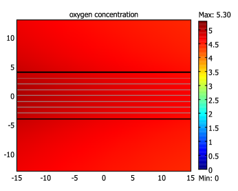
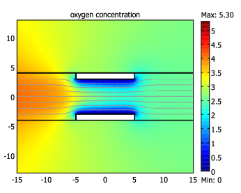
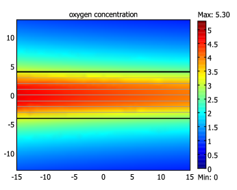
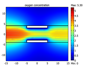
Figure 2: Oxygen concentration in the tissue and plasma within the vessel. Each diagram shows a cross section through the vessel and surrounding tissue of length $30\,\mbox{$\mu$m}$. Typically, this length of vessel contains about 4 cells. The left plots are for the vessel without robots. The right plots include the 10-micron ringset with pumps, which occupies the circumferential volume indicated by the white rectangles next to the vessel wall. The top and bottom plots are for the low and high demand scenarios of Table 2, respectively. Fluid in the vessel flows from left to right. Distances along the sides of each plot are indicated in microns and concentrations on the color bars are in units of $10^{22}\,\mbox{molecule}/\mbox{m}^{3}$. The horizontal black lines are the vessel walls and the gray curves inside the vessel are fluid flow streamlines.

Fig. 2 shows the distribution of oxygen in the tissue and plasma in the vessel near the robots. The robots reduce the local oxygen concentration far more than the surrounding tissue, as seen by comparing with the vessel without robots. Most of the extra oxygen used by the robots comes from the passing blood cells, which have about 100 times the oxygen concentration of the plasma. Within the vessel with the robots, the concentration in the plasma is lowest in the fluid next to the robots. Downstream of the robots is a recovery region where the concentration increases a bit as cells respond to the abruptly lowered concentration near the robots. In the low demand scenario, the concentration in the vessel just downstream of the robots is somewhat lower than in the surrounding tissue. Thus in this region, the net movement of oxygen is from the tissue into the vessel, where the fluid motion transports the oxygen somewhat downstream before it diffuses back into the tissue. In effect, part of the oxygen entering the vessel travels through the tissue around robots to the downstream section of the vessel, in contrast to the pattern without robots where oxygen is always moving from the vessel into the surrounding tissue. The streamlines in Fig. 2 show that the laminar flow speeds up as the fluid passes through the narrower vessel section where the robots are stationed.

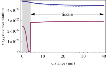
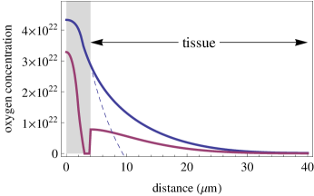
Figure 3: Oxygen concentration, in $\mbox{molecule}/\mbox{m}^{3}$, along a radial cross section from the center of the vessel to the outer edge of the tissue region. The cross section is in the middle of the modeled section of vessel and tissue, corresponding to a vertical line in the center of each plot of Fig. 2. The gray area indicates the interior of the vessel. The left and right plots correspond to the low and high demand scenarios of Table 2. In each plot, the upper curve is for the vessel without robots and the lower curve is for the vessel containing the $10\,\mbox{$\mu$m}$ ringset with pumps. For comparison, the dashed curves are solutions to the Krogh model [50] corresponding to the vessel without robots.

Fig. 3 gives another view of how the robots affect the oxygen concentration in the surrounding tissue. The concentration is zero at the robot surface facing into the vessel. The robots decrease the oxygen concentration somewhat but do not affect tissue power generation much since the concentration remains well above the threshold where power generation drops significantly, i.e., $K_{\mbox{\scriptsize tissue}}$ given in Table 1. However, at large distances from the vessel in the high demand scenario oxygen concentration is low enough to significantly decrease tissue power production. This low level of oxygen also occurs when there are no robots.

Fig. 3 includes comparison with the simpler Krogh model of oxygen transport to tissue from vessels without robots [50]. The Krogh model assumes constant power density in the tissue and no diffusion along the vessel direction in the tissue. For the low demand scenario, the Krogh model results are close to those from our model. However in the high demand case, the Krogh model has oxygen concentration drop to zero about $10\,\mbox{$\mu$m}$ from the vessel, due to the unrealistic assumption of constant power use rather than the decrease in power use at low concentrations given by Eq. (6).

Oxygen flux to the robots ranges from about $10^{19}$ to $10^{20}\,\mbox{molecule}/\mbox{m}^{2}/\mbox{s}$ with the zero-concentration boundary condition. Estimates of pump capabilities are up to $10^{22}\,\mbox{molecule}/\mbox{m}^{2}/\mbox{s}$ [27], which is more than 100 times the actual flux to the robots. Such pumps could thereby maintain the zero concentration boundary condition. At an energy use of $10^{-20}\,\mbox{J}/\mbox{molecule}$ [27], the pumps would require about $1\,\mbox{pW}$ per robot to handle the incoming flux, slightly reducing the power benefit of the pumps. However, much of this pumping energy may be recoverable by adding a generator using the subsequent expansion of the reaction products to their lower partial pressure outside the robot [26].

3.1 Robot Power

This section describes the steady-state power available to the robots according to our model in various scenarios. We first discuss the average per robot power in the aggregate, for both high and low capacity cases, which also indicates the total power available to the aggregate as a whole. We then show how the power is distributed among the robots, based on their location in the ringset. Finally, we illustrate the qualitative features of these results in a simpler, analytically-solvable model to identify key scaling relationships between robot design choices and power availability.

3.1.1 Average Robot Power

robot power generation capacity	high capacity								low capacity
inlet concentration $C_{\mbox{\scriptsize$\mbox{O}_{2}$}}$ ($10^{22}\,/\mbox{m}^{3}$)	3				7				7
pressure gradient $\nabla p$ ($10^{5}\,\mbox{Pa}/\mbox{m}$)	1		5		1		5		1		5
tissue power demand $P^{\mbox{\scriptsize max}}_{\mbox{\scriptsize tissue}}$ ($\mbox{kW}/\mbox{m}^{3}$)	4	60	4	60	4	60	4	60	4	60	4	60
10-micron ringset (with pumps)	12	8	14	12	17	11	24	18	17	11	24	18
10-micron ringset (free diffusion)	11	7	12	10	15	10	22	16	6	3	8	6
1-micron ring (with pumps)	44	27	49	36	69	36	99	58	69	36	99	58
1-micron ring (free diffusion)	31	19	34	25	49	25	71	38	9	4	12	7

Table 4: Average per-robot power generation (in picowatts) in various scenarios. Free diffusion is the “no pumps” case. The values in bold correspond to the low and high demand scenarios of Table 2.

Table 4 gives the average power generated using the available oxygen, per robot within the aggregate. As expected, robots receive more oxygen and hence can generate more power when inlet concentration is high, fluid speed is high or tissue power demand is low. In the first two cases, the flow brings oxygen through the vessel more quickly; in the last case, surrounding tissue removes less oxygen. The less than 2-fold decrease in robot power generation in the face of a larger 2.5-fold decrease in $\mbox{O}_{2}$ inlet concentration from the arterial to the venous end of the capillary shows that robots extract more oxygen from red cells than these cells would normally release while passing the length of the vessel. Thus robots get some of their oxygen as “new oxygen” rather than just taking it from what the tissues would normally get. This is possible because in this case robots create steeper concentration gradients than the tissue does.

The 10-micron ringset with pumps produces about the same power in the low and high demand scenarios, consuming oxygen at $5\times 10^{9}\,\mbox{molecule}/\mbox{s}$.

Comparing the different aggregate sizes shows lower power generation, per robot, in the large aggregate compared to the small one. This arises from the competition among nearby robots for the oxygen. Nevertheless the larger aggregate, with ten times as many robots, generates several times as much power in aggregate as the smaller one. This difference identifies a design choice for aggregation: larger aggregates have more total power available but less on a per robot basis.

Robots using pumps generate only modestly more power than robots relying on diffusion alone in our high capacity design example (Section 2.5). In this case, for robots without pumps, the power generation site density, $\rho_{\mbox{\scriptsize react}}$, is sufficiently large that oxygen molecules diffusing into the robot are mostly consumed by the power generators near the surface of the robot before they have a chance to diffuse back out of the robot. For such robots, power generators far from the plasma-facing surface receive very little oxygen and hence do not add significantly to the robot power production.

Pumps give higher benefit for isolated rings of robots than for tightly clustered aggregates. Although not evaluated in the axially symmetric model used here, pumps may be even more significant for a single isolated robot on the vessel wall. Such a robot would not be competing with any other robots for the available oxygen, though would still compete with nearby tissue.

3.1.2 Low Capacity Robots

The low capacity robots have only $1/50^{th}$ the maximum power generating capability of the high capacity robots discussed above. Nevertheless, each robot’s maximum power is several times larger than the limit due to available oxygen. Thus pumps allow the robots to produce the same power as given in Table 4 for the high capacity robots. The pumps ensure the absorbed oxygen is completely used by the smaller number of reaction sites by increasing the concentration of oxygen within the robots so Eq. (5) gives the same power generation in spite of the smaller value of $\rho_{\mbox{\scriptsize react}}$.

On the other hand, the smaller number of reaction sites is a significant limitation for robots without pumps. Comparing with Table 4 shows pumps improve the average power by factors of about 3 and 8 for the 10 and 1-micron ringsets, respectively. Comparing with high capacity robots without pumps shows the factor of 50 reduction in reaction sites only reduces average power by factors of about 3 and 5 for the 10 and 1-micron ringsets, respectively. Thus the reaction sites in the low capacity scenario are used more effectively than in the high capacity robots: with a smaller number of sites, each site does not compete as much with nearby sites for the available oxygen.

Much of the power in robots without pumps is generated near the plasma-facing surface, where oxygen concentration is largest. In our case, the power for the high capacity robots is generated primarily within $100\,\mbox{nm}$ of the robot surface. This observation suggests that a design with power generating sites placed near this surface instead of uniformly throughout the robot volume, as we have assumed, could significantly improve power generation for robots without pumps. For example, placing all the reaction sites uniformly within the $1/50^{th}$ of the robot volume nearest the surface would increase the local reaction site density in that volume by a factor of 50. For low capacity robots, this placement would increase $\rho_{\mbox{\scriptsize react}}$ to the same value as the high capacity case, but only in a narrow volume, within $23\,\mbox{nm}$ of the surface with the robot geometry we use. Elsewhere in the robot with this design $\rho_{\mbox{\scriptsize react}}=0$. While we might expect this concentration to increase power significantly, in fact we find only a small increase (e.g., 12% for the 10-micron ringset in the low demand scenario). Thus concentrating the reaction sites near the plasma-facing surface does not offer much of a performance advantage.

3.1.3 Distribution of Power Among Robots

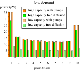
Figure 4: Steady-state power generation, in picowatts, for robots as a function of their position along the vessel wall, starting from those at the upstream end of the ringset (position 1) and continuing to those at the downstream end (position 10). The charts, corresponding to the low and high demand scenarios of Table 2, compare robots with pumps, absorbing all oxygen reaching them, with robots relying on free diffusion (i.e., without pumps), and high and low capacity robots. For robots with pumps, power for high and low capacity cases are the same.

While all robots in a single ring have the same power due to the assumption of axial symmetry, Fig. 4 shows that power varies with ring position in the 10-micron ringset. The robots at the upstream edge of the aggregate receive more oxygen than the other robots and hence produce more power. Power generation does not decrease monotonically along the vessel: robots at the downstream edge have somewhat more available oxygen than those in the middle of the aggregate since robots at the edge of the aggregate have less competition for oxygen. Fig. 4 shows significantly larger benefits of pumps at the edges of multi-ring aggregates than in their middle sections, especially in the low demand scenario.

In the scenarios described above, robots produce power from all the available oxygen. This is appropriate for applications requiring as much power as possible for the aggregate as a whole. At the other extreme, an application requiring the same behavior from all robots in the aggregate would be limited by the robots with the least available power. This would be the case for identical robots, all of which perform the same task and hence use the same power. In this case, the robots could increase performance by transferring power from those at the edges of the aggregate to those in the middle. Such transfer could take place after generation, e.g., via shared electric current, or prior to generation by transfer of oxygen among neighboring robots. However, such internal transfer would require additional hardware capabilities. For robots with pumps, an alternative transfer method is for robots near the edge of the aggregate to run their pumps at lower capacity and thus avoid collecting all the oxygen arriving at their surfaces. This uncollected oxygen would then be available for other robots, though some of this oxygen would be transported by the fluid past the robots or be captured by the tissue rather than other robots. This approach increases power to robots in the middle of the aggregate without requiring additional hardware for internal transfers between robots, but at the cost of somewhat lower total power for the aggregate. Increasing as much as possible the power to the robots with the least power leads to a uniform distribution of power among the robots.

To quantify the trade-off between total power and its uniformity among the robots, we consider all robots setting each of the pumps on their surfaces to operate at the same rate and the pumps uniformly distributed over the surface. This gives a uniform flux of oxygen over the entire surface of all the robots. The largest possible value for this uniform flux, and hence the largest power for the aggregate, occurs when the minimum oxygen concentration on the robot surfaces is zero – at that point, the robot whose surface includes the location of zero concentration cannot further increase its uniform flux. For example, in the low demand scenario the maximum value for this uniform flux is approximately $2.22\times 10^{19}\,\mbox{molecule}/\mbox{m}^{2}/\mbox{s}$. Compared to the situation in Fig. 4, this uniform flux gives significantly lower power (39% leading ring, 56% trailing ring) for the robots at the edges of the aggregate, somewhat lower power for robots in positions 2 and 3 (87% and 98%, respectively) and somewhat more power (ranging from 104% to 116%) for the other robots. The combination of these changes gives a total of $84\%$ of the power for the aggregate when every robot collects all the oxygen reaching its surface. The minimum power per robot increases from $12\,\mbox{pW}$ to $14\,\mbox{pW}$. Robots could slightly increase power by accepting some nonuniformity of flux over each surface while maintaining the same total flux to each robot. This would occur when the minimum oxygen concentration on the entire length of the robot surfaces in a particular robot ring is zero.

Using this approach to uniform power in practice would require the robots to determine the maximum rate they can operate their pumps while achieving uniform power distribution. This rate would vary with tissue demand, and also over time as cells pass the robots. A simple control protocol is for each robot to adjust its pump rate up or down according to whether its power generation is below or above that of its neighbors, respectively. When concentration reaches zero on one robot, increasing pump rate at that location would not increase power generation. Communicating information for this protocol is likely simpler than the hardware required to internally transfer power or oxygen among robots, but also requires each robot is able to measure its power generation rate. Such measurements and communication would give an effective control provided they operate rapidly compared to the time over which oxygen flux changes, e.g., as cells pass the robots on millisecond time scales. Longer reaction times could lead to oscillations or chaotic behavior [43].

A second approach to achieving a more uniform distribution of power is to space the robots at some distance from each other on the vessel wall. This approach would be suitable if the aggregated robots do not need physical contact to achieve their task. For example, somewhat separating the robots would allow a relatively small number to span a distance along the vessel wall larger than the size of a single cell passing through the vessel. This aggregate would always have at least some robots between successive cells. Communicating sensor readings among the robots would then ensure the response, e.g., releasing chemicals, is not affected by misleading sensor values due to the passage of a single cell, giving greater stability and reliability without the need for delaying response due to averaging over sensor readings as an alternative approach to accounting for passing cells. Another example for spaced robots is for directional acoustic communication, at distances of about $100\,\mbox{$\mu$m}$ [27]. Achieving directional control requires acoustic sources extending over distances comparable to or larger than the sound wavelength. Plausible acoustic communication between nanorobots involves wavelengths of tens of microns [27].

As a quantitative example of the benefit of spacing robots in the context of our axially symmetric model, we consider a set of rings of robots spaced apart along the vessel wall. When the distance between successive rings is sufficiently large, the power for each ring would be close to that of the isolated 1-micron ring given in Table 4. For example, the power for the low demand scenario in the 1-micron ring of high-capacity robots decreases from $69\,\mbox{pW}$ at high inlet concentration to $44\,\mbox{pW}$ at low inlet concentration, which spans the range of power for a modest number of widely spaced 1-micron rings within a single vessel. As described in Section 3.3, oxygen absorption by robots can affect concentration over a few tens of microns upstream of those robots. Thus separating robot rings by, say, $100\,\mbox{$\mu$m}$ will give power close to that of the isolated rings, with a gradual decrease in power for successive rings due to the decreasing cell saturation along the vessel.

A third approach to reducing variation in robot power, on average, is through changing pump rates in time. For example, adjacent nanorobot rings could operate with counterphased 50% duty cycles, with one ring and its second nearest neighbor ring using pumps while the intervening nearest neighbor has its pumps off and does not absorb oxygen. The alternating rings of robots would switch pumps on and off. In this case, robots would have larger power than seen in Fig. 4 for the half of the time they are active, and zero power for the other half. This temporal approach would not be suitable for tasks requiring all robots to have the same power simultaneously, but would be useful for tasks requiring higher burst power from robots throughout the aggregate where the robots are unable to store oxygen or power for later use. Provided the duty cycle is sufficiently long, our steady-state model can quantify the resulting power distribution. For example, in the low demand scenario, total flux for the aggregate is 79% of that when every robot collects all the oxygen reaching its surface, and the minimum power per robot drops from $12\,\mbox{pW}$ to $10\,\mbox{pW}$. Thus, when averaged over the duty cycle, this temporal technique reduces total power without benefiting the robots receiving the minimum power. In this case, the temporal approach does not improve minimum robot power (on average) since the power gain to a robot while its neighbors are off is less than a factor of 2, which does not compensate for the loss due to each robot being off for half the time. Applying the steady-state model to this temporal variation in robot activity requires the duty cycle be long enough for the system to reach steady-state behavior after each switch between the active subset of robots, and that the switching time is short compared to the duty cycle so most of the robots’ power arises during the steady-state portions of the cycle between switching. Diffusion provides one lower bound on this time: when neighboring robots switch pumps from on to off or vice versa, the characteristic diffusion time for oxygen over the distance between next nearest neighbors (one micron) is about $0.1\,\mbox{ms}$. Adjustments in cell saturation for the 1-micron shift in the location of the active robots between each half of the duty cycle is a further limitation on the duty cycle time for the validity of the steady-state model, though this is likely to be minimal since the cells are separated from the robots by the plasma gap in the fluid. Since the steady-state model averages over the position of passing cells, another lower bound on the duty cycle arises from the time for a cell to pass the robots. From the speeds in Table 1, this time is at least $100\,\mbox{ms}$.

3.1.4 Analytical Model for an Isolated Spherical Robot

The dependence of robot power on design parameters described above may appear contrary to simple intuitions. First, one might expect that the 10-micron ringset, with ten times the surface area in contact with the plasma, would absorb about ten times as much oxygen as the 1-micron ring. Instead we find only about a factor of 2 to 4 increase. Second, the benefit of pumps, less than a factor of 2 for the high capacity robots, may seem surprisingly small. Third, the low capacity robots, with $1/50^{th}$ the reaction sites of the high capacity robots, nevertheless generate about $1/5^{th}$ as much power as high capacity robots in the case with no pumps. And finally, in spite of the higher concentration near the robot surface than deep inside the robot when there are no pumps, increasing the reaction site density by placing all the reaction sites near the robot surface gives little benefit. While the specific values of these designs depend on the geometry and environment used in our model, these general features of small robots obtaining power through diffusion apply in other situations as well.

In this section we illustrate how these consequences of design choices arise in the context of a scenario for which the diffusion equation has a simple analytic solution, thereby identifying key physical effects leading to these behaviors. Specifically, we consider an isolated spherical robot of radius $a$ in a stationary fluid with oxygen concentration $C$ far from the sphere.

Such a sphere with a fully absorbing surface collects oxygen at a rate $4\pi D_{\mbox{\scriptsize$\mbox{O}_{2}$}}aC$ [10]. This expression illustrates a key property of diffusive capture: the rate depends not on the object’s surface area but on its size. This behavior, which also applies to other shapes [10], arises because while larger objects have greater surface areas they also encounter smaller concentration gradients. As a quantitative example, taking the sphere to have the same volume as the robot, i.e., $(4/3)\pi a^{3}=V_{\mbox{\scriptsize robot}}$ given in Table 3, the oxygen absorbed by the sphere generates $320$ and $750\,\mbox{pW}$ for $C$ equal to the low and high inlet oxygen concentrations in the plasma from Table 1, respectively. These power values are larger than for robots on the vessel wall described above. Unlike the sphere in a stationary fluid, the aggregated robots compete with each other for the oxygen, the fluid moves some of the oxygen past the robots before they have a chance to absorb it, and the surrounding tissue also consumes some of the oxygen. The replenishment of oxygen from the passing blood cells is not sufficient to counterbalance these effects.

The spherical robot also indicates the benefit of pumps. The fully absorbing sphere, with a zero concentration boundary condition at the surface, corresponds to using pumps. For robots without pumps, an approximation to Eq. (5) allows a simple solution. Specifically, since the Michaelis-Menten constant for the robot power generators, $K$, is much larger than the oxygen concentrations (e.g., as seen in Fig. 2), robot power generation from Eq. (5) is approximately $P_{\mbox{\scriptsize robot}}\approx(e\rho_{\mbox{\scriptsize react}}r/K)C_{\mbox{\scriptsize$\mbox{O}_{2}$}}$. Dividing by $e/6$ gives the oxygen consumption rate density as $\gamma C_{\mbox{\scriptsize$\mbox{O}_{2}$}}$ where $\gamma=6\rho_{\mbox{\scriptsize react}}r/K$. Solving the diffusion equation, Eq. (1), for a sphere in a stationary fluid with concentration $C$ far from the sphere, with free diffusion through the sphere’s surface and reaction rate density $\gamma C_{\mbox{\scriptsize$\mbox{O}_{2}$}}$ inside the sphere, gives the rate oxygen is absorbed by the sphere (and hence reacted to produce power) as [41] $4\pi D_{\mbox{\scriptsize$\mbox{O}_{2}$}}C(a-\mu\tanh(a/\mu))$ where $\mu=\sqrt{D_{\mbox{\scriptsize$\mbox{O}_{2}$}}/\gamma}$. Thus free diffusion produces a fraction

$$f_{\mu}=1-\frac{\mu}{a}\tanh\left(\frac{a}{\mu}\right)$$ (10)

of the power produced by the fully absorbing sphere. The distance $\mu$ is roughly the average distance an oxygen molecule diffuses in the time a power generation site consumes an oxygen molecule. When a freely diffusing molecule inside the robot has a high chance to diffuse out of the robot before it reacts ($\mu$ large compared to $a$), $f_{\mu}$ is small so pumps provide a significant increase in power. Conversely, when $\mu$ is small compared to $a$, pumps provide little benefit: the large number of reaction sites ensure the robot consumes almost all the diffusing oxygen reaching its surface.

This argument illustrates a tradeoff between using pumps to keep oxygen within the robot and the number of power generators. In particular, if internal reaction sites are easy to implement, then robots with many reaction sites and no pumps would be a reasonable design choice. Conversely, if reaction sites are difficult to implement while pumps are easy, then robots with pumps and few reaction sites would be a better choice.

A caveat for robots with few power generating sites is that Eq. (10) applies when oxygen consumption is linear in the concentration, as given by $\gamma C_{\mbox{\scriptsize$\mbox{O}_{2}$}}$. This expression allows arbitrarily increasing the reaction rate by increasing the concentration, no matter how small the number of reaction sites. This linearity is a good approximation of Eq. (5) only when $C_{\mbox{\scriptsize$\mbox{O}_{2}$}}\ll K$. At larger concentrations the power density saturates at $e\rho_{\mbox{\scriptsize react}}r$. When $\rho_{\mbox{\scriptsize react}}$ is sufficiently small, this limit is below the power that could be produced from all the oxygen that a fully absorbing sphere collects. Thus, in practice, the benefit of using pumps estimated from the linear reaction rate, $G=f_{\mu}^{-1}$, is limited by this bound when $\rho_{\mbox{\scriptsize react}}$ is small.

As an example, for a spherical robot with the high capacity reaction site density of Table 3, $\gamma=1.8\times 10^{4}/\mbox{s}$ and $\mu=0.33\,\mbox{$\mu$m}$, with the fairly modest benefit of pumps $G=2.0$. The low capacity robots have $\gamma=360/\mbox{s}$ and $\mu=2.4\,\mbox{$\mu$m}$ with $G=42$. In this case, the limit due to the maximum reaction rate of Eq. (5) applies, somewhat limiting the benefit of pumps to a factor of $34$, but pumps still offer considerable benefit. These values for the benefits of pumps are somewhat larger than seen with our model for robots on the vessel wall. Nevertheless, the spherical example identifies the key physical properties influencing power generation with and without pumps, and how they vary with robot design choices.

Eq. (10) also illustrates why power in the low capacity robots is not as small as one might expect based on the reduction in reaction sites by a factor of 50. While the value of $\gamma$ is proportional to $\rho_{\mbox{\scriptsize react}}$, the typical diffusion distance $\mu$ varies as $1/\sqrt{\rho_{\mbox{\scriptsize react}}}$, so a decrease in reaction sites by a factor of 50 only increases $\mu$ by about a factor of 7. The square root dependence arises from the fundamental property of diffusion: typical distance a diffusing particle travels grows only with the square root of the time. The modest change in diffusion distance, combined with Eq. (10), gives a smaller decrease in power than the factor of 50 decrease in capacity. The low capacity robot has higher concentrations throughout the sphere, so each reaction site operates more rapidly than in the high capacity case. This increase partially offsets the decrease in the number of reaction sites.

Without pumps, the higher oxygen concentration near the sphere’s surface than near its center means much of the power generation takes place close to the surface. Thus we can expect an increase in power by placing reaction sites close to the surface rather than uniformly distributed throughout the sphere. Consistent with the results from the model described in Section 2, evaluating Eq. (1) with the reaction confined to a spherical shell shows only a modest benefit compared to a uniform distribution. The benefit is larger for a thinner shell and is determined by the same ratio, $a/\mu$, appearing in Eq. (10). In particular, the largest benefit of using a thin shell, only $12\%$, occurs for $a/\mu\approx 3.5$. The parameters for the high and low capacity robots are somewhat below this optimal value, giving only $10\%$ and less than $1\%$ benefit from a thin shell, respectively, for the sphere. These modest improvements correspond to the small benefits of using a thin shell seen in the solution to our model for both high and low capacity robots. Hence the solution of Eq. (1) for the sphere illustrates how, with a fixed number of reaction sites, concentrating them near the robot surface provides only limited benefit. The benefit of the higher reaction site density in the shell is almost entirely offset by the shorter distance molecules need to diffuse to escape from the thin reactive region. That is, the benefit of placing all the reaction sites in a thin shell arises from two competing effects. When $\mu$ is large (low capacity) the concentration is only slightly higher near the surface than well inside the sphere. So there is little benefit from placing the reaction sites closer to the surface. On the other hand, when $\mu$ is small (high capacity), even uniformly distributed reaction sites manage to consume most of the arriving oxygen, giving near-zero concentration at the surface of the sphere and little scope for further improvement by concentrating the reaction sites. Thus the largest, though still modest, benefit for a shell design is for intermediate values of $a/\mu$.

3.2 Oxygen Replenishment from Passing Cells

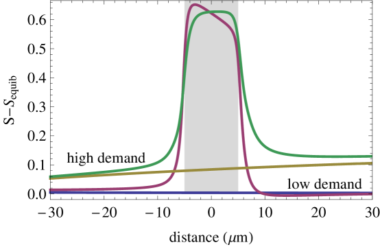
Figure 5: Deviation from equilibrium oxygen saturation in cells, $S-S_{\mbox{\scriptsize equib}}$, along the boundary between the cell and cell-free portions of the fluid illustrated in Fig. 1, as a function of distance along that boundary. A deviation of zero indicates the oxygen held in the cells is in perfect equilibrium with the surrounding plasma. Saturation ranges between 0 and 1. The curves correspond to the low and high demand scenarios of Table 2, when robots are present (upper curves) or absent (lower curves). For the vessel without robots and low demand, $S-S_{\mbox{\scriptsize equib}}$ is indistinguishable from zero on the scale of the plot. The gray band indicates the 10-micron length of the vessel wall in which the robots are stationed, within the 60-micron length of the capillary illustrated.

The high power density of the robots creates a steep gradient of oxygen concentration in the plasma. Thus, unlike the minor role for nonequilibrium oxygen release in tissue [67], the small size of the robots makes passing red cells vary significantly from equilibrium with the concentration in the plasma. Fig. 5 illustrates this behavior, using one measure of the amount of disequilibration: the difference between saturation $S$ and the equilibrium value $S_{\mbox{\scriptsize equib}}$ corresponding to the local concentration of oxygen in the plasma, as given by Eq. (2). We compare with a vessel without robots, in which the blood cells remain close to equilibrium.

Fig. 5 shows that the kinetics of oxygen release from red cells plays an important role in limiting the oxygen available to the robots. However, the region of significant disequilibration is fairly small, extending only a few microns from the robots.

3.3 Tissue Power and Heating

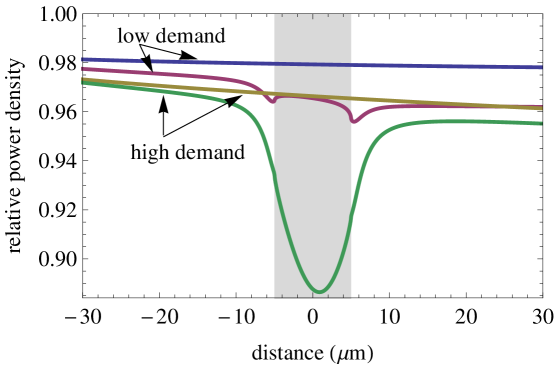
Figure 6: Power density in tissue next to the vessel wall relative to maximum demand, i.e., the ratio $P_{\mbox{\scriptsize tissue}}/P^{\mbox{\scriptsize max}}_{\mbox{\scriptsize tissue}}$ from Eq. (6), as a function of position along the vessel. The curves are for the low and high demand scenarios of Table 2. The two lines at the top are for the vessel without robots and the lower curves are for the 10-micron ringsets. In each case, the curve with higher values corresponds to the low power demand scenario. The gray band indicates the 10-micron length of the vessel wall in which the robots are stationed, within the 60-micron length of the capillary illustrated.

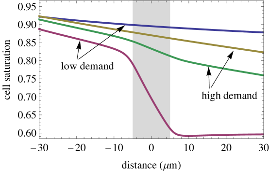
Figure 7: Cell saturation $S$ as a function of distance along the vessel. Saturation ranges between 0 and 1. The curves correspond to the low and high demand scenarios of Table 2, with the upper curves of each pair corresponding to a vessel without robots. The gray band indicates the 10-micron length of the vessel wall in which the robots are stationed, within the 60-micron length of the capillary illustrated.

The robots affect tissue power in two ways. First, the robots compete for oxygen with nearby tissue. Second, the robots consume oxygen from passing blood cells, thereby leaving less for tissue downstream of the robots.

For the effect on nearby tissue, Fig. 6 shows how tissue power density varies next to the vessel wall. In the vessel without robots, power density declines slightly with distance along the vessel as the tissue consumes oxygen from the blood. The total reduction in tissue power density is fairly modest, less than 10% even for high power demand in the tissues. The relative reduction is less for tissue at larger distances from the vessel, though such tissue has lower power generation due to less oxygen reaching tissue far from the vessel. This reduction arises both from direct competition by the robots for available oxygen and the physical blockage of the capillary wall, forcing surrounding tissue to rely on oxygen diffusing a longer distance from unblocked sections of the wall. In the low demand case, direct competition is the major factor, as seen by the dips in the power density at each end of the aggregate, where the absorbing flux is highest. In the high demand case, the tissue’s consumption reduces the amount of oxygen diffusing through the tissue on either side of the aggregate, giving the larger drop in tissue power density in the middle of the aggregate.

For longer range consequences, Fig. 7 shows how the oxygen saturation in the blood cells changes as they pass the robots. Slowly moving cells (in the low demand scenario) are substantially depleted while passing the robots, even though tissue power demand in this scenario is low. This depletion arises from the cells remaining near the robots a relatively long time as cells move slowly with the fluid. The resulting saturation shown in the figure, around $0.6$, is below the equilibrium saturation ($S=0.7$) for typical concentrations at the venous end of capillaries, given in Table 1. Thus in the low demand scenario, the robots remove more oxygen from passing cells than occurs during their full transit of a vessel containing no robots. In this scenario, the tissue has low power demand, so the depletion of oxygen from the cells may have limited effect on tissue along the vessel downstream of the robots. However, this reduction could significantly limit the number of robots that can be simultaneously present inside a given capillary.

Another observation from Fig. 7 is a significant decrease in cell saturation a short distance upstream of the robots in the low demand scenario. We can understand this behavior in terms of the Peclet number, which characterizes the relative importance of convection and diffusion over various distances [79]. In particular, $D/v_{\rm{avg}}$ is the distance at which diffusion and convection have about the same effect on mass transport in a moving fluid. At significantly longer distances, convection is the dominant effect and absorption of oxygen at a given location in the vessel has little effect on upstream concentrations over such distances. In our scenarios, $D/v_{\rm{avg}}$ ranges from $\sim 2\,\mbox{$\mu$m}$ (high demand) to $\sim 10\,\mbox{$\mu$m}$ (low demand). Thus the oxygen concentration in the plasma is significantly affected by the robots over a few tens of microns upstream of their location. Cell saturation remains close to equilibrium in this upstream region (Fig. 5), hence the reduced oxygen concentration in the plasma lowers cell saturation in this region upstream of the robots (Fig. 7). This distance is also relevant for spacing rings of robots far enough apart to achieve nearly uniform power, as described in Section 3.1.3.

The devices in this example have a volume of $V_{\mbox{\scriptsize robot}}\approx 1\,\mbox{$\mu$m}^{3}$ so the robot power generation corresponds to power densities around $10^{7}\,\mbox{W}/\mbox{m}^{3}$, several orders of magnitude larger than power densities in tissue, raising concerns of possible significant tissue heating by the robots. However, for the isolated aggregate used in this scenario, waste heat due to the robots’ power generation is rapidly removed, resulting in negligible maximum temperature elevation of about $10^{-4}\,{}^{\circ}\mathrm{C}$.

3.4 Fluid Flow and Forces on the Robots

The robots change the fluid flow by constricting the vessel. With the same pressure difference as a vessel without robots, as used in our model, this constriction results in somewhat lower flow speed through the vessel. Specifically, the one and ten-micron long aggregates reduce flow speed by 6% and 20%, respectively.

The fluid moving past the robots exerts a force on them. To remain on the wall the robots must resist this force through their attachment to the vessel wall [27]. This force is a combination of pressure difference, between the upstream and downstream ends of the aggregate, and viscous drag. For the laminar flow the force $f$ is linear in the pressure gradient $\nabla p$ imposed on the vessel: $f=a\nabla p$ where $a=1.56\times 10^{-15}\,\mbox{m}^{3}$ and $5.02\times 10^{-16}\,\mbox{m}^{3}$ for the $10\,\mbox{$\mu$m}$ and $1\,\mbox{$\mu$m}$ ringsets, respectively. For example, the flow imposes a force of $160\,\mbox{pN}$ on the $10\,\mbox{$\mu$m}$ ringset when the pressure gradient is $10^{5}\,\mbox{Pa}/\mbox{m}$. The $10\,\mbox{$\mu$m}$ ringset experiences about three times the force of the $1\,\mbox{$\mu$m}$ ring, but covers ten times the surface area. Thus the larger aggregate requires about one-third the attachment force per robot. Applied forces can affect cells [22]. In particular, endothelial cells use forces as a trigger for new vessel growth [21], which is important for modeling changes in the vessels over longer time scales than we consider in this paper [82].

4 Discussion

The scenarios of this paper illustrate how various physical properties affect robot power generation. Robots about one micron in size positioned in rings on capillary walls could generate a few tens of picowatts in steady state from oxygen and glucose scavenged locally from the bloodstream. Aggregates can combine their oxygen intake for tasks requiring higher sustained power generation. The resulting high power densities do not significantly heat the surrounding tissue, but do introduce steep gradients in oxygen concentration due to the relatively slow reaction kinetics of oxygen release from red cells. The robots reduce oxygen concentration in nearby tissues, but generally not enough to significantly affect tissue power generation.

The fraction of the generated power available for useful activity within the robot depends on the efficiency of the glucose engine design, with $\sim 50\%$ a reasonable estimate for fuel cells [27]. The robots will have $5\mbox{--}30\,\mbox{pW}$ of usable steady-state power while on the vessel wall. As one indication of the usefulness of this power for computation, current nanoscale electronics and sensors have an energy cost per logic operation or sensor switching event of a few hundred $k_{B}T$ [89]. While future technology should enable lower energy use [27], even with $500\,k_{B}T\approx 2\times 10^{-18}J$ the available power from circulating oxygen could support several million computational operations per second. At the size of these robots, significant movements of blood cells and chemical transport occur on millisecond time scales. Thus the power could support thousands of computational operations, e.g., for chemical pattern recognition, in this time frame. The aggregated robots could share sensor information and CPU cycles, thereby increasing this capability by a factor of tens to hundreds.

The robots need not generate power as fast as they receive oxygen, but could instead store oxygen received over time to enable bursts of activity as they detect events of interest. Robots with pumps have a significant advantage in burst-power applications because pumps enable long-term high-concentration onboard gas accumulation to support brief periods of near maximal power generation. As an example, in our scenarios individual robots with pumps receive about $10^{8}\,\mbox{molecule}/\mbox{s}$. If instead of using this oxygen for immediate power generation, the robot stored the oxygen received over one second, it would have enough to run the power generators at near maximal rate (giving about $10^{4}\,\mbox{pW}$) for several milliseconds. By contrast, robots without pumps would only have a modest benefit from oxygen diffusing into the robot, achieving a concentration equal to the ambient concentration in the surrounding plasma as given in Table 1. This concentration could only support generating several hundred picowatts for about a tenth of a millisecond. Thus while pumps may give only modest improvement for steady-state power generation, they can significantly increase power available in short bursts.

Our model could be extended to estimate the amount of onboard storage that would be required to avoid pathological conditions related to $\mbox{O}_{2}$ competition between tissues and nanorobots. In particular, larger aggregates would deplete oxygen over longer distances for which diffusion through the tissue from upstream of the robots would be insufficient. Furthermore, larger aggregates of tightly-spaced robots would block transport from the capillary into the surrounding tissue even if the robots did not use much oxygen. Onboard oxygen storage would allow higher transient power densities for the robots, though this could lead to heating issues for larger aggregates. To estimate the potential for onboard storage, a ringset containing 200 robots with volume $200V_{\mbox{\scriptsize robot}}\approx 220\,\mbox{$\mu$m}^{3}$ of which 10% is devoted to compressed $\mbox{O}_{2}$ storage at 1000 atmospheres at body temperature can store about $5\times 10^{11}$ molecules of $\mbox{O}_{2}$ in the aggregate. The incoming flow in the capillary provides about $0.2\mbox{--}1\times 10^{11}$ molecules per second, depending on the flow speed, of which about $1/4$ to $1/2$ is available to the tissue and robots. This means the oxygen stored in the aggregate is equivalent to only several seconds of oxygen delivery through the vessel. Thus oxygen storage in the robots themselves can not significantly increase mission duration, though such storage might be useful for short-term (i.e., a few seconds) load leveling functions (e.g., maintaining function during temporary capillary blockage due to white cell passage).

Alternatively, the aggregated robots could have oxygen supplemented with a modest circulating population of respirocytes [26], i.e., $1\,\mbox{$\mu$m}$ spherical robots able to carry oxygen to tissues far more effectively than red blood cells. Such robots would continuously and entirely eliminate any oxygen depletion regions in the tissue due to robot power generation, and allow higher robot power generation since oxygen would no longer be such a limiting factor. Such machines could not only carry significantly more oxygen than red blood cells, but would also respond more quickly to abrupt decreases in partial pressure due to consumption by aggregated robots on vessel walls. For example, sensors should be able to detect the drop in concentration of the size we see near the robots – e.g., $(3\mbox{ to }2)\times 10^{22}\,\mbox{molecule}/\mbox{m}^{3}$ (or about $40-20\,\mbox{mmHg}$) – within a millisecond [27]. This time is short enough that the machines will have moved only about a micron and so will still be near the robots. Once they detect the pressure drop, the machines could release oxygen rapidly, up to $1.5\times 10^{8}\,\mbox{molecule}/\mbox{s}$ [26], while passing near the aggregated robots. However, in practice the release rate is constrained by the effervescence limit in plasma to about $2.5\times 10^{7}\,\mbox{molecule}/\mbox{s}$ [27]. An interesting question for future work is evaluating how much of this released oxygen reaches the robots on the vessel wall, which will depend on how close to the vessel wall the fluid places the respirocytes. In this situation, aggregated robots could also communicate [27] to passing respirocytes to activate or suppress their oxygen delivery, depending on the task at hand. Thus both the oxygen handling capabilities of respirocytes, giving faster kinetics than red cells and larger storage capacity, and the possibility of communication provide examples of the flexibility of small devices with programmable control. Moreover, this scenario illustrates the benefits of mixing robots with differing hardware capabilities.

Our model considers static aggregates on vessel walls, but could be extended to study power availability for aggregates that move along the walls [25]. Another significant scenario is robots moving passively with the fluid, where they could draw oxygen from the surrounding plasma. The oxygen unloading model used here could evaluate how rapidly nearby cells would replenish oxygen in the plasma as the cells and robots move through the capillary.

We treat environmental parameters (e.g., fluid flow speed and tissue oxygen demand) as fixed by the surroundings. Beyond the local changes in the robots’ environment described by the model, sustained use of these robots could induce larger scale responses. For example, the increased use of oxygen by the robots could lead to increased blood flow, as occurs with, say, exercising muscles, by increased pressure to drive the fluid at higher speed or dilation of the vessels. The local oxygen deficits due to high robot power use are smaller in scale than higher tissue demand (e.g., from increased activity in a muscle). Thus an important open question is whether localized robot oxygen consumption over a long period of time can initiate a less localized response to increase flow in the vessels.

The possibility of large-scale responses to robot activity raises a broader issue for nanomedicine treatment design when technology allows altering the normal correlation among physical quantities used for signalling in the body [27, 30]. An example at larger scales is the response to low oxygen mediated by excess carbon dioxide in the blood, which can lead to edema and other difficulties for people at high altitudes [72]. In terms of downstream consequences of the robots’ oxygen use, low saturation of cells leaving an isolated capillary should not be a problem because the bulk of oxygen exchange occurs in the capillary bed, not in the larger collecting vessels. However, cells reaching low saturation before exiting the capillary would produce localized anoxia in the tissue near the end of the capillary. This could be relieved in part by oxygen diffusion from neighboring tissue cells if the anoxic region is not too large or too severe. Specific effects of such localized anoxia remain to be fully identified. Whole capillaries subjected to ischemic conditions over a period of days remodel themselves, e.g., by adding new vascular branches and by increasing the tortuosity of existing vessels [5]. This observed behavior is likely to be a localized (i.e., cell-level) response, hence we might expect such a response if a portion of a capillary downstream of the robots was driven into ischemic conditions. There could also be a localized inflammatory response to a large enough number of capillary-wall endothelial cells under stress, especially for cells stressed to the point of apoptosis, but moderate ischemia alone seems unlikely to generate this response [15]. Various chemicals (e.g., adrenalin) make the heart pump faster and thus drive the blood at higher speed. Other chemicals (such as NO, PGD2 and LTD4) dilate the vessels. These chemicals can produce significant activity in the endothelial cells that line (and thus form the tube geometry of) the capillary vessel, so their influence can be fairly direct and quick [78, 74]. Similarly, a large robot population constantly drawing excess oxygen supply could induce elevated erythropoietin secretion (if unregulated by the robots), increasing red cell production in the erythroid marrow [26, 23].

Direct heating is not a problem with aggregates of the size considered here, in spite of their high power density compared to tissue. For the large aggregate we examined (tightly covering $10\,\mbox{$\mu$m}$ along the vessel wall), oxygen diffusion through the tissue from regions upstream and downstream of the robots provided oxygen to the tissue outside the section of the vessel blocked by the robots. Larger aggregates, especially if tightly packed, would significantly reduce oxygen in the tissues even if the robots used little power themselves, simply due to their covering the vessel wall over a long enough distance that diffusion through the tissue from unblocked regions is no longer effective. The inducement of nonlinear tissue thermal responses (e.g., inflammation or fever) due to the heat generated by larger aggregates or multiple aggregates in nearby capillaries is an important question for future work.

Nanorobots parked or crawling along the luminal surface of the vessel may activate mechanosensory responses from the endothelial cells across whose surfaces the nanorobots touch [29]. If the aggregates cover a long section of the vessel wall, they could produce local edemas since narrowing of the vessels by the presence of the nanorobots increases local pressure gradients and fluid velocities. While we focus on a single aggregate in one microscopic vessel, additional issues arise if a large population of circulating robots form many aggregates. In that case, the multiple aggregates will increase hydrodynamic resistance throughout the fluidic circuit. Thus the robots could make the heart work slightly harder to pump fluid against the slightly higher load. Moreover, if robot aggregates detach from the wall without complete disaggregation, these smaller aggregates moving in the blood may be large enough to block a small vessel.

The scenarios examined in this paper can suggest suitable controls to distribute power when robots aggregate. Moreover, power control decisions interact with the choices made for the aggregation process. For example, if the task requires a certain amount of total power for the aggregate (e.g., as a computation hub) then the aggregation self-assembly protocol would depend on how much oxygen is available, e.g., to make a larger aggregate in vessels with less available oxygen, or recruit more passing robots when the task needs more power. An example of this latter case could be if aggregates are used as computation hubs to validate responses to rare events: when local sensor readings indicate the possibility of such an event, the aggregate could temporarily recruit additional robots to increase power and computational capability for evaluating whether those readings warrant initiating treatment.

Another approach to designing controls for teams of robots is the formalism of partially observable Markov processes [16, 75]. This formalism allows for arbitrarily complex computations among the robots to update their beliefs about their environment and other robots. Unfortunately this generality leads to intractable computations for determining optimal control processes. For the situations we studied, the power constraints on capillary wall-resident microscopic robots operating with oxygen available in vivo means the local rules must be simple. Including this constraint in the formalism could allow it to identify feasible control choices for large aggregates of microscopic robots in these situations.

The power constraints from our model could provide useful parameters for less detailed models of the behavior of large numbers of robots in the circulation in the context of the scenarios examined in this paper. In particular, power limits the computation, communication and locomotion capabilities of the robots. These constraints could be incorporated in simplified models, such as cellular automata approaches to robot behavior. These automata are a set of simple machines, typically arranged on a regular lattice. Each machine is capable of communicating with its neighbors on the lattice and updates its internal state based on a simple rule. For example, a two-dimensional scenario shows how robots could assemble structures [4] using local rules. Such models can help understand structures formed at various scales through simple local rules and some random motions [91, 35]. A related analysis technique considers swarms [13], i.e., groups of many simple machines or biological organisms such as ants. In these systems, individuals use simple rules to determine their behavior from information about a limited portion of their environment and neighboring individuals. Typically, individuals in swarms are not constrained to have a fixed set of neighbors but instead continually change their neighbors as they move. Swarm models are well-suited to microscopic robots with their limited physical and computational capabilities and large numbers. Most swarm studies focus on macroscopic robots or behaviors in abstract spaces [33]. In spite of the simplified physics, these studies show how local interactions among robots lead to various collective behaviors [85] and provide broad design guidelines. A step toward more realistic, though still tractable, models of large aggregates could incorporate the power constraints from the model presented in this paper.

In addition to evaluating performance of hypothetical medical nanorobots, theoretical studies identifying tradeoffs between control complexity and hardware capabilities can aid future fabrication. One example is the design complexity of the robot’s fuel acquisition and utilization systems. For steady-state operation on vessel walls, we found limited benefit of pumps over free diffusion when numerous onboard power generators can be employed. In such cases, our results indicate that a design without pumps does not sacrifice much performance. More generally, control can compensate for limited hardware (e.g., sensor errors or power limitations), providing design freedom to simplify the hardware through additional control programs. Thus the studies could help determine minimum hardware performance capabilities needed to provide robust systems-level behavior.

A key challenge for robot design studies based on approximate models is validating the results. In our case, the most significant approximations are the treatment of cells as an averaged component in the fluid and the lumped-model kinetics for oxygen unloading. With increased computational power, numerical solution of more accurate models could test the validity of these approximations. As technology advances to constructing early versions of microscopic robots, experimental evaluations will supplement theoretical studies. One such experiment is operating the robots in manufactured microfluidic channels [79]. This would test the robots’ ability to aggregate at chemically defined locations and generate power reliably from known chemical concentrations in the fluid. After such in vitro experiments, early in vivo tests could involve robots acting as passive sensors in the circulatory system and aggregating at chemically distinctive locations. Such nanorobots will be useful not only as diagnostic tools and sophisticated extensions to drug delivery capabilities [3], but also as an aid to develop robot designs and control methods for more active tasks.

References

- [1] Comsol multiphysics. comsol.com, 2008.
- [2] Ann Ager. Inflammation: Border crossings. Nature, 421:703–705, 2003.
- [3] Thresa M. Allen and Pieter R. Cullis. Drug delivery systems: Entering the mainstream. Science, 303:1818–1822, 2004.
- [4] Daniel Arbuckle and Aristides A. G. Requicha. Active self-assembly. In Proc. of the IEEE Intl. Conf. on Robotics and Automation, pages 896–901, 2004.
- [5] A. M. Bailey, T. J. O’Neill 4th, C. E. Morris, and S. M. Peirce. Arteriolar remodeling following ischemic injury extends from capillary to large arteriole in the microcirculation. Microcirculation, 15:389–404, 2008.
- [6] Jie Bao, Keiji Furumoto, Kimitoshi Fukunaga, and Katsumi Nakao. A kinetic study on air oxidation of glucose catalyzed by immobilized glucose oxidase for production of calcium gluconate. Biochemical Engineering Journal, 8:91–102, 2001.
- [7] Amelia Barreiro et al. Subnanometer motion of cargos driven by thermal gradients along carbon nanotubes. Science, 320:775–778, 2008.
- [8] Denise Bechet et al. Nanoparticles as vehicles for delivery of photodynamic therapy agents. Trends in Biotechnology, 26:612–621, 2008.
- [9] Yaakov Benenson, Binyamin Gil, Uri Ben-Dor, Rivka Adar, and Ehud Shapiro. An autonomous molecular computer for logical control of gene expression. Nature, 429:423–429, 2004.
- [10] Howard C. Berg. Random Walks in Biology. Princeton Univ. Press, 2nd edition, 1993.
- [11] Howard C. Berg and Edward M. Purcell. Physics of chemoreception. Biophysical Journal, 20:193–219, 1977.
- [12] Jose Berna et al. Macroscopic transport by synthetic molecular machines. Nature Materials, 4:704–710, 2005.
- [13] Eric Bonabeau, Marco Dorigo, and Guy Theraulaz. Swarm Intelligence: From Natural to Artificial Systems. Oxford University Press, Oxford, 1999.
- [14] George E. Briggs and John B. S. Haldane. A note on the kinetics of enzyme action. Biochemical Journal, 19:338–339, 1925.
- [15] M. D. Brown, J. Kent, C. J. Kelsall, M. Milkiewicz, and O. Hudlicka. Remodeling in the microcirculation of rat skeletal muscle during chronic ischemia. Microcirculation, 10:179–191, 2003.
- [16] Anthony R. Cassandra, Leslie Pack Kaelbling, and Michael L. Littman. Acting optimally in partially observable stochastic domains. In Proc. of the 12th Natl. Conf. on Artificial Intelligence (AAAI94), pages 1023–1028, Menlo Park, CA, 1994. AAAI Press.
- [17] Swades K. Chaudhuri and Derek R. Lovley. Electricity generation by direct oxidation of glucose in mediatorless microbial fuel cells. Nature Biotechnology, 21:1229–1232, 2003.
- [18] Alfred Clark, Jr. et al. Oxygen delivery from red cells. Biophysical Journal, 47:171–181, 1985.
- [19] C. P. Collier et al. Electronically configurable molecular-based logic gates. Science, 285:391–394, 1999.
- [20] H. G. Craighead. Nanoelectromechanical systems. Science, 290:1532–1535, 2000.
- [21] Christophe F. Deroanne, Charles M. Lapiere, and Betty V. Nusgens. In vitro tubulogenesis of endothelial cells by relaxation of the coupling extracellular matrix-cytoskeleton. Cardiovascular Research, 49:647–658, 2001.
- [22] Dennis E. Discher, Paul Janmey, and Yu-li Wang. Tissue cells feel and respond to the stiffnes of their substrate. Science, 310:1139–1143, 2005.
- [23] A. J. Erslev and E. Beutler. Production and destruction of erythrocytes. In E. Beutler et al., editors, Williams Hematology, pages 425–441. McGraw-Hill, NY, 5th edition, 1995.
- [24] Alexander L. Fetter and John Dirk Walecka. Theoretical Mechanics of Particles and Continua. McGraw-Hill, NY, 1980.
- [25] Robert A. Freitas Jr. The end of heart disease. Technical report, Institute for Molecular Manufacturing, Palo Alto, CA, 1996.
- [26] Robert A. Freitas Jr. Exploratory design in medical nanotechnology: A mechanical artificial red cell. Artificial Cells, Blood Substitutes and Immobilization Biotechnology, 26:411–430, 1998.
- [27] Robert A. Freitas Jr. Nanomedicine, volume I: Basic Capabilities. Landes Bioscience, Georgetown, TX, 1999. Available at www.nanomedicine.com/NMI.htm.
- [28] Robert A. Freitas Jr. Clottocytes: Artificial mechanical platelets. Technical Report 18: Nanomedicine, Institute for Molecular Manufacturing, Palo Alto, CA, 2000.
- [29] Robert A. Freitas Jr. Nanomedicine, volume IIA: Biocompatibility. Landes Bioscience, Georgetown, TX, 2003. Available at www.nanomedicine.com/NMIIA.htm.
- [30] Robert A. Freitas Jr. Pharmacytes: An ideal vehicle for targeted drug delivery. Journal of Nanoscience and Nanotechnology, 6:2769–2775, 2006.
- [31] J. Fritz et al. Translating biomolecular recognition into nanomechanics. Science, 288:316–318, 2000.
- [32] Y. C. Fung. Biomechanics: Circulation. Springer, NY, 2nd edition, 1997.
- [33] V. Gazi and K. M. Passino. Stability analysis of social foraging swarms. IEEE Trans. on Systems, Man and Cybernetics, B34:539–557, 2004.
- [34] Cornelia Geers and Gerolf Gros. Carbon dioxide transport and carbonic anhydrase in blood and muscle. Physiological Reviews, 80:681–715, 2000.
- [35] Saul Griffith, Dan Goldwater, and Joseph M. Jacobson. Robotics: Self-replication from random parts. Nature, 437:636, 2005.
- [36] J. Halloy et al. Social integration of robots into groups of cockroaches to control self-organized choices. Science, 318:1155–1158, 2007.
- [37] Heiko Hamann, Heinz Worn, Karl Crailsheim, and Thomas Schmickl. Spatial macroscopic models of a bio-inspired robotic swarm algorithm. In Proc. of Intl. Conf. on Intelligent Robots and Systems (IROS 2008). INRIA, 2008.
- [38] Juan P. Hernandez-Ortiz, Christopher G. Stoltz, and Michael D. Graham. Transport and collective dynamics in suspensions of confined swimming particles. Physical Review Letters, 95:204501, 2005.
- [39] Ciaran Hill, Antonio Amodeo, Jean V. Joseph, and Hitendra R. H. Patel. Nano- and microrobotics: how far is the reality? Expert Review of Anticancer Therapy, 8:1891–1897, 2008.
- [40] Tad Hogg. Coordinating microscopic robots in viscous fluids. Autonomous Agents and Multi-Agent Systems, 14(3):271–305, 2007.
- [41] Tad Hogg. Diffusion to a spherical reactor. The Wolfram Demonstrations Project, February 2009. http://demonstrations.wolfram.com/DiffusionToASphericalReactor/.
- [42] Tad Hogg. Modeling microscopic chemical sensors in capillaries. The Open Nanomedicine Journal, 2:1–9, 2009.
- [43] Tad Hogg and Bernardo A. Huberman. Dynamics of large autonomous computational systems. In Kagan Tumer and David Wolpert, editors, Collectives and the Design of Complex Systems, pages 295–315. Springer, New York, 2004.
- [44] Tad Hogg and Philip J. Kuekes. Mobile microscopic sensors for high-resolution in vivo diagnostics. Nanomedicine: Nanotechnology, Biology, and Medicine, 2:239–247, 2006.
- [45] Tad Hogg and David W. Sretavan. Controlling tiny multi-scale robots for nerve repair. In Proc. of the 20th Natl. Conf. on Artificial Intelligence (AAAI2005), pages 1286–1291. AAAI Press, 2005.
- [46] Joe Howard. Molecular motors: Structural adaptations to cellular functions. Nature, 389:561–567, 1997.
- [47] George Karniadakis, Ali Beskok, and Narayan Aluru. Microflows and Nanoflows: Fundamentals and Simulation. Springer, Berlin, 2005.
- [48] Kenneth H. Keller. Effect of fluid shear on mass transport in flowing blood. In Proc. of Federation of American Societies for Experimental Biology, pages 1591–1599, Sept.-Oct. 1971.
- [49] Balazs L. Keszler, Istvan J. Majoros, and James R. Baker Jr. Molecular engineering in nanotechnology: Structure and composition of multifunctional devices for medical application. In Proc. of the Ninth Foresight Conference on Molecular Nanotechnology, 2001.
- [50] August Krogh. The number and distribution of capillaries in muscles with calculations of the oxygen pressure head necessary for supplying the tissue. J. of Physiology, 52:409–415, 1919.
- [51] S. K. Kufer et al. Single-molecule cut-and-paste surface assembly. Science, 319:594–596, 2008.
- [52] Scott P. Leary, Charles Y. Liu, and Michael L. J. Apuzzo. Toward the emergence of nanoneurosurgery: Part iii-nanomedicine: Targeted nanotherapy, nanosurgery, and progress toward the realization of nanoneurosurgery. Neurosurgery, 58:1009–1026, 2006.
- [53] Kristina Lerman, Aram Galstyan, Alcherio Martinoli, and Auke Jan Ijspeert. A macroscopic analytical model of collaboration in distributed robotic systems. Artificial Life, 7:375–393, 2001.
- [54] Rodolfo R. Llinas et al. Neuro-vascular central nervous recording/stimulating system: Using nanotechnology probes. J. of Nanoparticle Research, 7:111–127, 2005.
- [55] Bruce E. Logan et al. Electricity generation from cysteine in a microbial fuel cell. Water Research, 39:942–952, 2005.
- [56] Moustafa Malki, Antonio L. De Lacey, Nuria Rodríguez, Ricardo Amils, and Victor M. Fernandez. Preferential use of an anode as an electron acceptor by an acidophilic bacterium in the presence of oxygen. Applied and Environmental Microbiology, 74:4472–4476, 2008.
- [57] Thomas E. Mallouk and Ayusman Sen. Powering nanorobots. Scientific American, 300(5):72–77, May 2009.
- [58] James H. Marden and Lee R. Allen. Molecules, muscles, and machines: Universal performance characteristics of motors. Proceedings of the National Academy of Science USA, 99:4161–4166, 2002.
- [59] Sylvain Martel. The coming invasion of the medical nanorobots. Nanotechnology Perceptions, 3:165–173, 2007.
- [60] Sylvain Martel et al. Flagellated bacterial nanorobots for medical interventions in the human body. In Proc. of 2nd IEEE Conf. on Biomedical Robotics and Biomechatronics, pages 264–269, 2008.
- [61] Benjamin Mauroy. Following red blood cells in a pulmonary capillary. ESAIM Proceedings, 23:48–65, 2008.
- [62] B. J. McGuire and T. W. Secomb. A theoretical model for oxygen transport in skeletal muscle under conditions of high oxygen demand. Journal of Applied Physiology, 91:2255–2265, 2001.
- [63] Don Monroe. Micromedicine to the rescue. Communications of the ACM, 52:13–15, June 2009.
- [64] Carlo Montemagno and George Bachand. Constructing nanomechanical devices powered by biomolecular motors. Nanotechnology, 10:225–231, 1999.
- [65] Kelly Morris. Macrodoctor, come meet the nanodoctors. The Lancet, 357:778, March 10 2001.
- [66] NIH. National Institutes of Health roadmap: Nanomedicine, 2003. Available at nihroadmap.nih.gov/nanomedicine/index.asp.
- [67] Aleksander S. Popel. Theory of oxygen transport to tissue. Critical Reviews in Biomedical Engineering, 17:257–321, 1989.
- [68] Rachela Popovtzer et al. Targeted gold nanoparticles enable molecular CT imaging of cancer. Nano Letters, 8:4593–4596, 2008.
- [69] C. Pozrikidis. Axisymmetric motion of a file of red blood cells through capillaries. Physics of Fluids, 17:031503, 2005.
- [70] E. M. Purcell. Life at low Reynolds number. American Journal of Physics, 45:3–11, 1977.
- [71] Ingmar H. Riedel et al. A self-organized vortex array of hydrodynamically entrained sperm cells. Science, 309:300–303, 2005.
- [72] Robert B. Schoene. Illnesses at high altitude. Chest, 134:402–416, 2008.
- [73] T. W. Secomb, R. Hsu, and A. R. Pries. Motion of red blood cells in a capillary with an endothelial surface layer: effect of flow velocity. American J. of Physiology: Heart and Circulatory Physiology, 281:H629–H636, 2001.
- [74] K. Sekar. Inhaled nitric oxide in term and preterm infants. J. of Perinatology, 26(1):S4–7, discussion S22–23, May 2006.
- [75] Sven Seuken and Shlomo Zilberstein. Formal models and algorithms for decentralized decision making under uncertainty. Autonomous Agents and Multi-Agent Systems, 17:190–250, 2008.
- [76] Frederick H. Silver. Biological Materials: Structure, Mechanical Properties, and Modeling of Soft Tissues. New York Univ. Press, NY, 1987.
- [77] Ricky K. Soong et al. Powering an inorganic nanodevice with a biomolecular motor. Science, 290:1555–1558, 2000.
- [78] N. A. Soter et al. Local effects of synthetic leukotrienes (LTC4, LTD4, LTE4, and LTB4) in human skin. J. of Investigative Dermatology, 80:115–119, 1983.
- [79] Todd M. Squires and Stephen R. Quake. Microfluidics: Fluid physics at the nanoliter scale. Reviews of Modern Physics, 77:977–1026, 2005.
- [80] D. Sretavan, W. Chang, C. Keller, and M. Kliot. Microscale surgery on axons for nerve injury treatment. Neurosurgery, 57(4):635–646, 2005.
- [81] W. G. Strang and G. J. Fix. An Analysis of the Finite Element Method. Prentice-Hall, Englewood Cliffs, 1973.
- [82] Dominik Szczerba, Gabor Szekely, and Haymo Kurz. A multiphysics model of capillary growth and remodeling. In V. N. Alexandrov et al., editors, Proc. of ICCS, Part II, pages 86–93, Berlin, 2006. Springer.
- [83] Robert Tucker, Parag Katira, and Henry Hess. Herding nanotransporters: Localized activation via release and sequestration of control molecules. Nano Letters, 8:221–226, 2008.
- [84] A. Vadapalli, D. Goldman, and A. S. Popel. Calculations of oxygen transport by red blood cells and hemoglobin solutions in capillaries. Artificial Cells, Blood Substitutes and Immobilization Biotechnology, 30:157–188, 2002.
- [85] Tamas Vicsek et al. Novel type of phase transition in a system of self-driven particles. Physical Review Letters, 75:1226–1229, 1995.
- [86] Tuan Vo-Dinh, Paul Kasili, and Musundi Wabuyele. Nanoprobes and nanobiosensors for monitoring and imaging individual living cells. Nanomedicine: Nanotechnology, Biology, and Medicine, 2:22–30, 2006.
- [87] Steven Vogel. Life in Moving Fluids. Princeton Univ. Press, 2nd edition, 1994.
- [88] Tania Q. Vu et al. Activation of membrane receptors by a neurotransmitter conjugate designed for surface attachment. Biomaterials, 26:1895–1903, 2005.
- [89] S.-Y. Wang and R. Stanley Williams, editors. Nanoelectronics, volume 80, New York, March 2005. Springer. Special issue of Applied Physics A.
- [90] Xudong Wang et al. Direct-current nanogenerator driven by ultrasonic waves. Science, 316:102–105, 2007.
- [91] George M. Whitesides and Bartosz Grzybowski. Self-assembly at all scales. Science, 295:2418–2421, 2002.
- [92] Maung Nyan Win and Christina D. Smolke. Higher-order cellular information processing with synthetic RNA devices. Science, 322:456–460, 2008.