A Ferguson - Klass - LePage series representation of
multistable multifractional motions and related processes

Abstract

The study of non-stationary processes whose local form has controlled properties is a fruitful and important area of research, both in theory and applications. In [9], a particular way of constructing such processes was investigated, leading in particular to multifractional multistable processes, which were built using sums over Poisson processes. We present here a different construction of these processes, based on the Ferguson - Klass - LePage series representation of stable processes. We consider various particular cases of interest, including multistable Lévy motion, multistable reverse Ornstein-Uhlenbeck process, log-fractional multistable motion and linear multistable multifractional motion. We also show that the processes defined here have the same finite dimensional distributions as the corresponding processes constructed in [9]. Finally, we display numerical experiments showing graphs of synthesized paths of such processes.

Keywords: localisable processes, stable processes, Ferguson - Klass - LePage series representation, multifractional processes.

1 Introduction

This work deals with a general method for building stochastic processes for which certain aspects of the local form are prescribed. We will mainly be interested here in local Hölder regularity and local intensity of jumps, but our construction allows in principle to control other properties that could be of interest. Our approach is in the same spirit as the one proposed in [9], but it uses different methods. In particular, in [9], multistable processes, that is localisable processes which are locally $\alpha$-stable, but where the index of stability $\alpha$ varies with time, were constructed using sums over Poisson processes. We present here an alternative construction of such processes, based on the Ferguson - Klass - LePage series representation of stable stochastic processes [10, 13, 14]. This representation is a powerful tool for the study of various aspects of stable processes, see for instance [3, 18]. A comprehensive reference for the properties of this representation that will be needed here is [19].

Stochastic processes where the local Hölder regularity varies with a parameter $t$ are interesting both from a theoretical and practical point of view. A well-known example is multifractional Brownian motion (mBm), where the Hurst index $h$ of fractional Brownian motion [12, 15] is replaced by a functional parameter $h(t)$, permitting the Hölder exponent to vary in a prescribed manner [1, 2, 11, 16]. This allows in addition local regularity and long range dependence to be decoupled to give sample paths that are both highly irregular and highly correlated, a useful feature for instance in terrain or TCP traffic modeling.

However, local regularity, as measured by the Hölder exponent, is not the only local feature of a process that is useful in theory and applications. Jump characteristics also need to be accounted for, e.g. for studying processes with paths in $D({\bf R})$ (the space of càdlàg functions, i.e. functions which are continuous on the right and have left limits at all $t\in T$). This has applications for instance in the modeling of financial or medical data. Stable non-Gaussian processes yield relevant models for data containing discontinuities, with the stability index $\alpha$ controlling the distribution of jumps.

Just for the same reason why it is interesting to consider stochastic processes whose local Hölder exponent changes in a controlled manner, tractable models where the “jump intensity” $\alpha$ is allowed to vary in time are needed, for instance to obtain a more accurate description of some aspects of the local structure of functions in $D({\bf R})$.

The approach described in this work allows in particular to construct processes where both $h$ and $\alpha$ evolve in time in a prescribed way. Having two functional parameters allows to finely tune the local properties of these processes. This may prove useful to model two distinct aspects of financial risk, to describe epileptic episodes in EEG where for some periods there may be only small jumps and at other instants very large ones, or to study textured images where both Hölder regularity and the distribution of discontinuities vary.

Let us now recall the definition of a localisable process [6, 7]: $Y=\{Y(t):t\in{\bf R}\}$ is said to be $h-$localisable at $u$ if there exists an $h\in{\bf R}$ and a non-trivial limiting process $Y_{u}^{\prime}$ such that

$$\lim_{r\to 0}\frac{Y(u+rt)-Y(u)}{r^{h}}=Y_{u}^{\prime}(t).$$ (1.1)

(Note $Y_{u}^{\prime}$ may and in general will vary with $u$.) When the limit exits, $Y_{u}^{\prime}=\{Y_{u}^{\prime}(t):t\in{\bf R}\}$ is termed the local form or tangent process of $Y$ at $u$ (see [2, 16] for similar notions). The limit (1.1) may be taken in several ways. In this work, we will only deal with the case where convergence occurs in finite dimensional distributions (equality in finite dimensional distributions is denoted $\stackrel{{\scriptstyle fdd}}{{=}}$). When convergence takes place in distribution, the process is called strongly $h$-localisable (equality in distributions is denoted $\stackrel{{\scriptstyle d}}{{=}}$).

As mentioned above, a now classical example is multifractional Brownian motion $Y$ which “looks like” index-$h(u)$ fractional Brownian motion close to time $u$ but where $h(u)$ varies, that is

$$\lim_{r\to 0}\frac{Y(u+rt)-Y(u)}{r^{h}}=B_{h(u)}(t)$$ (1.2)

where $B_{h}$ is index-$h$ fractional Brownian motion. A generalization of mBm, where the Gaussian measure is replaced by an $\alpha$-stable one, leads to multifractional stable processes, where the local form is an $h(u)$-self-similar linear $\alpha$-stable motion [20, 21].

The $h$-local form $Y_{u}^{\prime}$ at $u$, if it exists, must be $h$-self-similar, that is $Y_{u}^{\prime}(rt)\stackrel{{\scriptstyle d}}{{=}}r^{h}Y_{u}^{\prime}(t)$ for $r>0$. In addition, as shown in [6, 7], under quite general conditions, $Y_{u}^{\prime}$ must also have stationary increments at almost all $u$ at which there is strong localisability. Thus, typical local forms are self-similar with stationary increments (sssi), that is $r^{-h}(Y_{u}^{\prime}(u+rt)-Y_{u}^{\prime}(u))\stackrel{{\scriptstyle d}}{{=}}Y_{u}^{\prime}(t)$ for all $u$ and $r>0$. Conversely, all sssi processes are localisable. Classes of known sssi processes include fractional Brownian motion, linear fractional stable motion and $\alpha$-stable Lévy motion, see [5, 19].

Similarly to [9], our method for constructing localisable processes is to make use of stochastic fields $\{X(t,v),(t,v)\in{\bf R}^{2}\}$, where $t$ is time, and where the process $t\mapsto X(t,v)$ is localisable for all $v$. This field will allow to control the local form of a ‘diagonal’ process $Y=\{X(t,t):t\in{\bf R}\}$. For instance, in the case of mBm, $X$ will be a field of fractional Brownian motions, i.e. $X(t,v)=B_{h(v)}(t)$, where $h$ is a smooth function of $v$ ranging in $[a,b]\subset(0,1)$. This is the approach that was used originally in [1] for studying mBm. From a heuristic point of view, taking the diagonal of such a stochastic field constructs a new process with local form depending on $t$ by piecing together known localisable processes. In other words, we shall use random fields $\{X(t,v):(t,v)\in{\bf R}^{2}\}$ such that for each $v$ the local form $X_{v}^{\prime}(\cdot,v)$ of $X(\cdot,v)$ at $v$ is the desired local form $Y_{v}^{\prime}$ of $Y$ at $v$. An easy situation is when, for each $v$, the process $\{X(t,v):t\in{\bf R}\}$ is sssi, since this automatically entails localisability.

It is clear that, in this approach, the structure of $X(\cdot,v)$ for $v$ in a neighbourhood of $u$ will be crucial to determine the local behaviour of $Y$ near $u$. A simple way to control this structure is to define the random field as an integral or sum of functions that depend on $t$ and $v$ with respect to a single underlying random measure so as to provide the necessary correlations.

General criteria that guarantee the transference of localisability from the $X(\cdot,v)$ to $Y=\{X(t,t):t\in{\bf R}\}$ were obtained in [9]. We will make use of the following one:

Theorem 1.1

Let $U$ be an interval with $u$ an interior point. Suppose that for some $0<h<\eta$ the process $\{X(t,u),t\in U\}$ is $h$-localisable at $u\in U$ with local form $X_{u}^{\prime}(\cdot,u)$ and

$${\sf P}(|X(v,v)-X(v,u)|\geq|v-u|^{\eta})\to 0$$ (1.3)

as $v\to u$. Then $Y=\{X(t,t):t\in U\}$ is $h$-localisable at $u$ with $Y_{u}^{\prime}(\cdot)=X_{u}^{\prime}(\cdot,u)$.

In the sequel, we shall consider specific classes of random fields and use Theorem 1.1 to build localisable processes with interesting local properties. As a particular case, we will study multifractional multistable processes, where both the local Hölder regularity and intensity of jumps will evolve in a controlled manner.

The remaining of this article is organized as follows: we first collect some notations in section 2. We then build localisable processes using a series representation that yields the necessary flexibility required for our purpose. We need to distinguish between the situations where the underlying space is finite (section 3), or merely $\sigma-$ finite (section 4). In each case, we define a random field depending on a “kernel” $f$, and give conditions on $f$ ensuring localisability of the diagonal process. We then consider in section 5 some examples: multistable Lévy motion, multistable reverse Ornstein-Uhlenbeck process, log-fractional multistable motion and linear multistable multifractional motion. Section 6 is devoted to computing the finite dimensional distributions of our processes, and proving that they are the same as the ones of the corresponding processes constructed in [9]. Finally, section 7 displays graphs of certain localisable processes of interest, in particular multifractional multistable ones.

Before we proceed, we note that constructing localisable processes using a stochastic field composed of sssi processes is obviously not the only approach that one can think of. It is for instance possible to follow a rather different path and construct localisable processes from moving average ones by imposing conditions on the kernel defining the moving average. See [8] for details.

2 Notations

We refer the reader to the first chapters of [19] for basic notions on stable random variables and stable processes. In particular, recall that a process $\{X(t):t\in T\}$, where $T$ is generally a subinterval of ${\bf R}$, is called $\alpha$-stable $(0<\alpha\leq 2)$ if all its finite-dimensional distributions are $\alpha$-stable. Many stable processes admit a stochastic integral representation as follows. Write $S_{\alpha}(\sigma,\beta,\mu)$ for the $\alpha$-stable distribution with scale parameter $\sigma$, skewness $\beta$ and shift-parameter $\mu$; we will assume throughout that $\mu=0$. Let $(E,{\cal E},m)$ be a sigma-finite measure space. Taking $m$ as the control measure and $\beta:E\to[-1,1]$ a measurable function, this defines an $\alpha$-stable random measure $M$ on $E$ such that for $A\in{\cal E}$ we have that $M(A)\sim S_{\alpha}\left(m(A)^{1/\alpha},\int_{A}\beta(x)m(dx)/m(A),0\right)$. If $\beta=0$, the process is termed symmetric $\alpha$-stable, or $S\alpha S$.

Let

$${\cal F}_{\alpha}\equiv{\cal F}_{\alpha}(E,{\cal E},m)=\{f:f\mbox{ is measurable and }\|f\|_{\alpha}<\infty\},$$

where $\|\,\|_{\alpha}$ is the quasinorm (or norm if $1<\alpha\leq 2$) given by

$$\|f\|_{\alpha}=\left\{\begin{array}[]{cc}\left(\int_{E}|f(x)|^{\alpha}m(dx)\right)^{1/\alpha}&(\alpha\neq 1)\\ \int_{E}|f(x)|m(dx)+\int_{E}|f(x)\beta(x)\ln|f(x)||m(dx)&(\alpha=1)\end{array}\right.$$ (2.4)

The stochastic integral of $f\in{\cal F}_{\alpha}(E,{\cal E},m)$ with respect to $M$ then exists [19, Chapter 3] with

$$I(f)=\int_{E}f(x)M(dx)\sim S_{\alpha}(\sigma_{f},\beta_{f},0),$$ (2.5)

where

$$\sigma_{f}=\|f\|_{\alpha},\quad\beta_{f}=\frac{\int f(x)^{<\alpha>}\beta(x)m(dx)}{\|f\|_{\alpha}^{\alpha}},$$

and $a^{<b>}\equiv\mbox{sign}({a})|a|^{b}$, see [19, Section 3.4]. In particular,

$$\mbox{\sf E}|I(f)|^{p}=\left\{\begin{array}[]{cc}c(\alpha,\beta,p)\|f\|_{\alpha}^{p}&(0<p<\alpha)\\ \infty&(p\geq\alpha)\end{array}\right.$$ (2.6)

where $c(\alpha,\beta,p)<\infty$, see [19, Property 1.2.17].

In this work, we will only consider the symmetric case, i.e. we take $\beta\equiv 0$ for the remaining of the article. We believe most results should have a counterpart in the non-symmetric case, although the proofs would probably have to be much more involved.

3 A Ferguson - Klass - LePage series representation of localisable processes in the finite measure space case

A well-known representation of stable random variables is the Ferguson - Klass - LePage series one [3, 10, 13, 14, 18]. This representation is particularly adapted for our purpose since, as we shall see, it allows for easy generalization to the case of varying $\alpha$.

In this work, we will use the following version:

Theorem 3.2

([19, Theorem 3.10.1])

Let $(E,{\cal E},m)$ be a finite measure space, and $M$ be a symmetric $\alpha$-stable random measure with $\alpha\in(0,2)$ and finite control measure $m$. Let $(\Gamma_{i})_{i\geq 1}$ be a sequence of arrival times of a Poisson process with unit arrival time, $(V_{i})_{i\geq 1}$ be a sequence of i.i.d. random variables with distribution $\hat{m}=m/m(E)$ on $E$, and $(\gamma_{i})_{i\geq 1}$ be a sequence of i.i.d. random variables with distribution $P(\gamma_{i}=1)=P(\gamma_{i}=-1)=1/2$. Assume finally that the three sequences $(\Gamma_{i})_{i\geq 1}$, $(V_{i})_{i\geq 1}$, and $(\gamma_{i})_{i\geq 1}$ are independent. Then, for any $f\in{\cal F}_{\alpha}(E,{\cal E},m)$,

$$\int_{E}f(x)M(dx)\stackrel{{\scriptstyle d}}{{=}}\left(C_{\alpha}m(E)\right)^{1/\alpha}\sum_{i=1}^{\infty}\gamma_{i}\Gamma_{i}^{-1/\alpha}f(V_{i}),$$ (3.7)

where $C_{\alpha}:=\frac{1-\alpha}{\Gamma(2-\alpha)\cos(\pi\alpha/2)}$ for $\alpha\neq 1$, $C_{1}=2/\pi$ (Theorem 3.10.1 in [19] is more general, as it extends to non-symmetric stable processes, that are not considered here.) As mentioned above, a relevant feature of this representation for us is that the distributions of all random variables appearing in the sum are independent of $\alpha$. We will use (3.7) to contruct processes with varying $\alpha$ as described in the following Theorem.

Theorem 3.3

Let $(E,{\cal E},m)$ be a finite measure space. Let $\alpha$ be a $C^{1}$ function defined on ${\bf R}$ and ranging in $[c,d]\subset(0,2)$. Let $b$ be a $C^{1}$ function defined on ${\bf R}$. Let $f(t,u,.)$ be a family of functions such that, for all $(t,u)\in{\bf R}^{2}$, $f(t,u,.)\in{\cal F}_{\alpha(u)}(E,{\cal E},m)$. Let $(\Gamma_{i})_{i\geq 1}$ be a sequence of arrival times of a Poisson process with unit arrival time, $(V_{i})_{i\geq 1}$ be a sequence of i.i.d. random variables with distribution $\hat{m}=m/m(E)$ on $E$, and $(\gamma_{i})_{i\geq 1}$ be a sequence of i.i.d. random variables with distribution $P(\gamma_{i}=1)=P(\gamma_{i}=-1)=1/2$. Assume finally that the three sequences $(\Gamma_{i})_{i\geq 1}$, $(V_{i})_{i\geq 1}$, and $(\gamma_{i})_{i\geq 1}$ are independent. Consider the following random field:

$$X(t,u)=b(u)(m(E))^{1/\alpha(u)}C^{1/\alpha(u)}_{\alpha(u)}\sum_{i=1}^{\infty}\gamma_{i}\Gamma_{i}^{-1/\alpha(u)}f(t,u,V_{i}),$$ (3.8)

where $C_{\alpha}=\left(\int_{0}^{\infty}x^{-\alpha}\sin(x)dx\right)^{-1}$. Assume that $X(t,u)$ (as a process in $t$) is localisable at $u$ with exponent $h\in(0,1)$ and local form $X^{\prime}_{u}(t,u)$. Assume in addition that:

• (C1) The family of functions $v\to f(t,v,x)$ is differentiable for all $(v,t)$ in a neighbourhood of $u$ and almost all $x$ in $E$. The derivatives of $f$ with respect to $v$ are denoted by $f^{\prime}_{v}$.

• (C2) There exists $\varepsilon>0$ such that:

  $$\sup_{t\in B(u,\varepsilon)}\int_{E}\sup_{w\in B(u,\varepsilon)}(|f(t,w,x)|^{\alpha(w)})\hskip 2.84544pt\hat{m}(dx)<\infty.$$ (3.9)

• (C3) There exists $\varepsilon>0$ such that:

  $$\sup_{t\in B(u,\varepsilon)}\int_{E}\sup_{w\in B(u,\varepsilon)}(|f^{\prime}_{v}(t,w,x)|^{\alpha(w)})\hskip 2.84544pt\hat{m}(dx)<\infty.$$ (3.10)

• (C4) There exists $\varepsilon>0$ such that:

  $$\sup_{t\in B(u,\varepsilon)}\int_{E}\sup_{w\in B(u,\varepsilon)}\left[\left|f(t,w,x)\log|f(t,w,x)|\right|^{\alpha(w)}\right]\hskip 2.84544pt\hat{m}(dx)<\infty.$$ (3.11)

Then $Y(t)\equiv X(t,t)$ is localisable at $u$ with exponent $h$ and local form $Y^{\prime}_{u}(t)=X^{\prime}_{u}(t,u)$.

Proof

The function $u\mapsto C^{1/\alpha(u)}_{\alpha(u)}$ is $C^{1}$ since $\alpha(u)$ ranges in $[c,d]\subset(0,2)$. We shall denote $a(u)=b(u)(m(E))^{1/\alpha(u)}C^{1/\alpha(u)}_{\alpha(u)}$. The function $a$ is thus also $C^{1}$. We want to apply Theorem 1.1. With that in view, we estimate, for $v\in B(u,\varepsilon)$ (the ball centered at $u$ with radius $\varepsilon$),

$$X(v,v)-X(v,u)=:\sum_{i=1}^{\infty}\gamma_{i}(\Phi_{i}(v)-\Phi_{i}(u))+\sum_{i=1}^{\infty}\gamma_{i}(\Psi_{i}(v)-\Psi_{i}(u)),$$

where

$$\Phi_{i}(u)=a(u)i^{-1/\alpha(u)}f(v,u,V_{i})$$

and

$$\Psi_{i}(u)=a(u)\left(\Gamma_{i}^{-1/\alpha(u)}-i^{-1/\alpha(u)}\right)f(v,u,V_{i}).$$

The reason for introducing the $\Phi_{i}$ and the $\Psi_{i}$ is that the random variables $\Gamma_{i}$ are not independent, which complicates their study. We shall decompose the sum involving the $\Phi_{i}$ into series of independent random variables which will be dealt with using the three series theorem. The sum involving the $\Psi_{i}$ will be studied by taking advantage of the fact that, for large enough $i$, each $\Gamma_{i}$ is “close” to $i$ in some sense.

In the sequel, since only the values of $\alpha$ inside $B(u,\varepsilon)$ matter, we shall agree by convention that $c$ denotes in fact $\inf_{v\in B(u,\varepsilon)}\alpha(v)$ and likewise $d=\sup_{v\in B(u,\varepsilon)}\alpha(v)$. Note that, by decreasing $\varepsilon$, $d-c$ may be made arbitrarily small.

Thanks to the assumptions on $a$ and $f$, $\Phi_{i}$ and $\Psi_{i}$ are differentiable and one computes:

$$\Phi_{i}^{\prime}(u)=a^{\prime}(u)i^{-1/\alpha(u)}f(v,u,V_{i})+a(u)i^{-1/\alpha(u)}f^{\prime}_{u}(v,u,V_{i})+a(u)\frac{\alpha^{\prime}(u)}{\alpha(u)^{2}}\log(i)i^{-1/\alpha(u)}f(v,u,V_{i}),$$

and

$$\Psi_{i}^{\prime}(u)=a^{\prime}(u)\left(\Gamma_{i}^{-1/\alpha(u)}-i^{-1/\alpha(u)}\right)f(v,u,V_{i})+a(u)\left(\Gamma_{i}^{-1/\alpha(u)}-i^{-1/\alpha(u)}\right)f^{\prime}_{u}(v,u,V_{i})$$

$$+a(u)\frac{\alpha^{\prime}(u)}{\alpha(u)^{2}}\left(\log(\Gamma_{i})\Gamma_{i}^{-1/\alpha(u)}-\log(i)i^{-1/\alpha(u)}\right)f(v,u,V_{i}).$$

The mean value theorem yields that there exists a sequence of independent random numbers $w_{i}\in[u,v]$ (or $[v,u]$) and a sequence of random numbers $x_{i}\in[u,v]$ (or $[v,u]$) such that:

$$X(v,u)-X(v,v)=(u-v)\sum_{i=1}^{\infty}(Z_{i}^{1}+Z_{i}^{2}+Z_{i}^{3})+(u-v)\sum_{i=1}^{\infty}(Y_{i}^{1}+Y_{i}^{2}+Y_{i}^{3}),$$

where

$$Z_{i}^{1}=\gamma_{i}a^{\prime}(w_{i})i^{-1/\alpha(w_{i})}f(v,w_{i},V_{i}),$$

$$Z_{i}^{2}=\gamma_{i}a(w_{i})i^{-1/\alpha(w_{i})}f^{\prime}_{u}(v,w_{i},V_{i}),$$

$$Z_{i}^{3}=\gamma_{i}a(w_{i})\frac{\alpha^{\prime}(w_{i})}{\alpha(w_{i})^{2}}\log(i)i^{-1/\alpha(w_{i})}f(v,w_{i},V_{i}),$$

$$Y_{i}^{1}=\gamma_{i}a^{\prime}(x_{i})\left(\Gamma_{i}^{-1/\alpha(x_{i})}-i^{-1/\alpha(x_{i})}\right)f(v,x_{i},V_{i}),$$

$$Y_{i}^{2}=\gamma_{i}a(x_{i})\left(\Gamma_{i}^{-1/\alpha(x_{i})}-i^{-1/\alpha(x_{i})}\right)f^{\prime}_{u}(v,x_{i},V_{i}),$$

$$Y_{i}^{3}=\gamma_{i}a(x_{i})\frac{\alpha^{\prime}(x_{i})}{\alpha(x_{i})^{2}}\left(\log(\Gamma_{i})\Gamma_{i}^{-1/\alpha(x_{i})}-\log(i)i^{-1/\alpha(x_{i})}\right)f(v,x_{i},V_{i}).$$

Note that each $w_{i}$ depends on $a,f,\alpha,u,v,V_{i}$, but not on $\gamma_{i}$. This remark will be useful in the sequel.

The remainder of the proof is divided into four steps. The first step will apply the three-series theorem to show that each series $\sum_{i=1}^{\infty}\limits Z_{i}^{j},j=1,2,3,$ converges almost surely. In the second step, we will prove that $\sum_{i=1}^{\infty}\limits Y_{i}^{j}$ also converges almost surely for $j=1,2,3$. In the third step we will prove that condition (1.3) is verified by $\sum_{i=1}^{\infty}\limits Z_{i}^{j},j=1,2,3$. Finally, step four will prove the same thing for $\sum_{i=1}^{\infty}\limits Y_{i}^{j},j=1,2,3$.

First step: almost sure convergence of $\sum_{i=1}^{\infty}\limits Z_{i}^{j},j=1,2,3$.

Consider $Z^{1}=\sum_{i=1}^{\infty}\limits Z_{i}^{1}$. Fix $\lambda>0$. We shall deal successively with the three series involved the three-series theorem.

First series: $S_{1}=\sum_{i=1}^{\infty}\limits{\sf P}(|Z_{i}^{1}|>\lambda)$.

$${\sf P}(|Z_{i}^{1}|>\lambda) = {\sf P}\left(|f(v,w_{i},V_{i})|>\frac{\lambda i^{1/\alpha(w_{i})}}{|a^{\prime}(w_{i})|}\right)$$

$$\leq {\sf P}\left(|f(v,w_{i},V_{i})|^{\alpha(w_{i})}>i\inf_{w\in B(u,\varepsilon)}\left[\left(\frac{\lambda}{|a^{\prime}(w)|}\right)^{\alpha(w)}\right]\right).$$

Note that, since $a^{\prime}$ is bounded on the compact interval $[u,v]$, $K:=\inf_{w\in B(u,\varepsilon)}\left[\left(\frac{\lambda}{|a^{\prime}(w)|}\right)^{\alpha(w)}\right]$ is strictly positive.

$${\sf P}(|Z_{i}^{1}|>\lambda) \leq {\sf P}\left(\sup_{w\in B(u,\varepsilon)}|f(v,w,V_{i})|^{\alpha(w)}>Ki\right)$$

$$= {\sf P}\left(\sup_{w\in B(u,\varepsilon)}|f(v,w,V_{1})|^{\alpha(w)}>Ki\right).$$

Thus

$$\sum_{i=1}^{+\infty}{\sf P}(|Z_{i}^{1}|>\lambda) \leq \sum_{i=1}^{+\infty}{\sf P}\left(\sup_{w\in B(u,\varepsilon)}|f(v,w,V_{1})|^{\alpha(w)}>Ki\right)$$

$$\leq \frac{1}{K}\mbox{\sf E}\left[\sup_{w\in B(u,\varepsilon)}|f(v,w,V_{1})|^{\alpha(w)}\right]$$

$$\leq \frac{1}{K}\sup_{t\in B(u,\varepsilon)}\int_{E}\sup_{w\in B(u,\varepsilon)}(|f(t,w,x)|^{\alpha(w)})\hskip 2.84544pt\hat{m}(dx)$$

$$< +\infty$$

by (C2).

Second series: $S_{2}^{n}=\sum_{i=1}^{n}\limits\mbox{\sf E}(Z_{i}^{1}{\sf 1}{\sf l}{\sf\_}\{|Z_{i}^{1}|\leq\lambda\})$.

$$\mbox{\sf E}(Z_{i}^{1}{\sf 1}{\sf l}{\sf\_}\{|Z_{i}^{1}|\leq\lambda\}) = \mbox{\sf E}(\gamma_{i}a^{\prime}(w_{i})i^{-1/\alpha(w_{i})}f(v,w_{i},V_{i}){\sf 1}{\sf l}{\sf\_}\{|a^{\prime}(w_{i})i^{-1/\alpha(w_{i})}f(v,w_{i},V_{i})|\leq\lambda\})$$

$$= \mbox{\sf E}(\gamma_{i})\mbox{\sf E}(a^{\prime}(w_{i})i^{-1/\alpha(w_{i})}f(v,w_{i},V_{i}){\sf 1}{\sf l}{\sf\_}\{|a^{\prime}(w_{i})i^{-1/\alpha(w_{i})}f(v,w_{i},V_{i})|\leq\lambda\})$$

$$= 0,$$

where we have used the facts that $\gamma_{i}$ is independent of $w_{i},V_{i}$ and $\mbox{\sf E}(\gamma_{i})=0$. As a consequence, $\lim_{n\rightarrow+\infty}S_{2}^{n}=0$.

Third series: The final series we need to consider is $S_{3}=\sum_{i=1}^{\infty}\limits\mbox{\sf E}\left[(Z_{i}^{1}{\sf 1}{\sf l}{\sf\_}\{|Z_{i}^{1}|\leq 1\})^{2}\right]$. Take $\lambda=1$.

Let $\eta$ be such that $d<\eta<2$.

$$(Z_{i}^{1}{\sf 1}{\sf l}{\sf\_}\{|Z_{i}^{1}|\leq 1\})^{2} \leq |Z_{i}^{1}|^{\eta}{\sf 1}{\sf l}{\sf\_}\{|Z_{i}^{1}|\leq 1\}$$

$$\mbox{\sf E}\left[(Z_{i}^{1}{\sf 1}{\sf l}{\sf\_}\{|Z_{i}^{1}|\leq 1\})^{2}\right] \leq \mbox{\sf E}\left[|Z_{i}^{1}|^{\eta}{\sf 1}{\sf l}{\sf\_}\{|Z_{i}^{1}|\leq 1\}\right]$$

$$= \int_{0}^{+\infty}{\sf P}(|Z_{i}^{1}|^{\eta}{\sf 1}{\sf l}{\sf\_}\{|Z_{i}^{1}|\leq 1\}>x)dx$$

$$= \int_{0}^{1}{\sf P}(|Z_{i}^{1}|^{\eta}{\sf 1}{\sf l}{\sf\_}\{|Z_{i}^{1}|\leq 1\}>x)dx$$

$$\leq \int_{0}^{1}{\sf P}(|Z_{i}^{1}|^{\eta}>x)dx.$$

Now, for all $x$ in $(0,1)$,

$${\sf P}(|Z_{i}^{1}|^{\eta}>x) = {\sf P}(|Z_{i}^{1}|>x^{1/\eta})$$

$$\leq {\sf P}\left(|f(v,w_{i},V_{i})|^{\alpha(w_{i})}>i\frac{x^{\frac{\alpha(w_{i})}{\eta}}}{|a^{\prime}(w_{i})|^{\alpha(w_{i})}}\right)$$

$$\leq {\sf P}\left(\sup_{w\in B(u,\varepsilon)}|f(v,w,V_{i})|^{\alpha(w)}>K^{\prime}ix^{\frac{d}{\eta}}\right)$$

$$= {\sf P}\left(\sup_{w\in B(u,\varepsilon)}|f(v,w,V_{1})|^{\alpha(w)}>K^{\prime}ix^{\frac{d}{\eta}}\right),$$

where $K^{\prime}:=\inf_{w\in B(u,\varepsilon)}\left[\left(\frac{1}{|a^{\prime}(w)|}\right)^{\alpha(w)}\right]$ is strictly positive. Thus,

$$S_{3} \leq \int_{0}^{1}\sum_{i=1}^{\infty}{\sf P}\left(\sup_{w\in B(u,\varepsilon)}|f(v,w,V_{1})|^{\alpha(w)}>K^{\prime}ix^{\frac{d}{\eta}}\right)dx$$

$$\leq \int_{0}^{1}\frac{1}{K^{\prime}x^{\frac{d}{\eta}}}\mbox{\sf E}(\sup_{w\in B(u,\varepsilon)}|f(v,w,V_{1})|^{\alpha(w)})dx$$

$$\leq \frac{1}{K^{\prime}}\left(\sup_{t\in B(u,\varepsilon)}\int_{E}\sup_{w\in B(u,\varepsilon)}(|f(t,w,x)|^{\alpha(w)})\hskip 2.84544pt\hat{m}(dx)\right)\left(\int_{0}^{1}\frac{dx}{x^{\frac{d}{\eta}}}\right)$$

$$< +\infty.$$

The case of the $Z^{2}=\sum_{i=1}^{\infty}\limits Z_{i}^{2}$ is treated similarly, since the conditions required on $(a^{\prime},f)$ in the proof above are also satisfied by $(a,f^{\prime}_{u})$.

Consider finally $Z^{3}=\sum_{i=1}^{\infty}\limits Z_{i}^{3}$. Fix $\lambda>0$.

First series: $S_{1}=\sum_{i=1}^{\infty}\limits{\sf P}(|Z_{i}^{3}|>\lambda)$.

$${\sf P}(|Z_{i}^{3}|>\lambda) = {\sf P}\left(|f(v,w_{i},V_{i})|>\frac{\lambda\alpha(w_{i})^{2}i^{1/\alpha(w_{i})}}{|a(w_{i})\alpha^{\prime}(w_{i})|\log i}\right)$$

$$\leq {\sf P}\left(|f(v,w_{i},V_{i})|^{\alpha(w_{i})}>K^{\prime\prime}\frac{i}{(\log i)^{\alpha(w_{i})}}\right),$$

where $K^{\prime\prime}:=\inf_{w\in B(u,\varepsilon)}\left[\left(\frac{\lambda\alpha(w)^{2}}{|a(w)\alpha^{\prime}(w)|}\right)^{\alpha(w)}\right]$ is strictly positive by the assumptions on $a,\alpha$ and $\alpha^{\prime}$. In the sequel, $K$ will always denote a finite positive constant, that may however change from line to line.

Let $g_{i}(x)=\frac{Kx}{(\log x)^{\alpha(w_{i})}}$ for $x\geq 1$ and $i\in\mathbb{N}^{*}$. For $x$ large enough and for all $i$, $g_{i}$ is strictly increasing and $\lim_{x\rightarrow+\infty}g_{i}(x)=+\infty$. For $z$ large enough (independently of $i$),

$$g_{i}(z(\log z)^{\alpha(w_{i})}) = \frac{Kz(\log z)^{\alpha(w_{i})}}{(\log z+\alpha(w_{i})\log\log z)^{\alpha(w_{i})}}$$

$$\geq \frac{Kz}{2}.$$

Let $A>e$ be such that: $\forall z\geq A,\forall i\in\mathbb{N}^{*},g_{i}^{-1}(z)\leq\frac{z}{K}(\log z)^{\alpha(w_{i})}$.

Let $U_{i}=|f(v,w_{i},V_{i})|^{\alpha(w_{i})}$.

$${\sf P}(|Z_{i}^{3}|>\lambda) \leq {\sf P}(U_{i}>K\frac{i}{(\log i)^{\alpha(w_{i})}})$$

$$\leq {\sf P}(\left(\{U_{i}<A\}\cap\{U_{i}>K\frac{i}{(\log i)^{\alpha(w_{i})}}\}\right)\cup\left(\{U_{i}\geq A\}\cap\{g_{i}^{-1}(U_{i})>i\}\right))$$

$$\leq {\sf P}(A>U_{i}>K\frac{i}{(\log i)^{d}})+{\sf P}(\{U_{i}\geq A\}\cap\{U_{i}|\log U_{i}|^{\alpha(w_{i})}>Ki\})$$

$$\leq {\sf P}(A>U_{i}>K\frac{i}{(\log i)^{d}})+{\sf P}(U_{i}|\log U_{i}|^{\alpha(w_{i})}>Ki)$$

$$\leq {\sf P}(A>U_{i}>K\frac{i}{(\log i)^{d}})+{\sf P}(\sup_{w\in B(u,\varepsilon)}[|f(v,w,V_{1})\log|f(v,w,V_{1})||^{\alpha(w)}]>\frac{K}{d^{d}}i).$$

On the one hand, ${\sf P}(A>U_{i}>K\frac{i}{(\log i)^{d}})$ vanishes for i large. On the other hand, by (C3),

$$\sum_{i}{\sf P}\left(\sup_{w\in B(u,\varepsilon)}[|f(v,w,V_{1})\log|f(v,w,V_{1})||^{\alpha(w)}]>\frac{K}{d^{d}}i\right) \leq$$

$$\frac{d^{d}}{K}\mbox{\sf E}\left(\sup_{w\in B(u,\varepsilon)}[|f(v,w,V_{1})\log|f(v,w,V_{1})||^{\alpha(w)}]\right)<+\infty$$

and thus $S_{1}<+\infty$.

Second series: $S_{2}^{n}=\sum_{i=1}^{n}\limits\mbox{\sf E}(Z_{i}^{3}{\sf 1}{\sf l}{\sf\_}\{|Z_{i}^{3}|\leq\lambda\})$.

For the same reason as in the case of $Z_{i}^{1}$ (i.e. $\gamma_{i}$ is independent of $w_{i},V_{i}$), $S_{2}^{n}=0$, $\forall n$.

Third series: $S_{3}=\sum_{i=1}^{\infty}\limits\mbox{\sf E}((Z_{i}^{3}{\sf 1}{\sf l}{\sf\_}\{|Z_{i}^{3}|\leq 1\})^{2})$. Take again $\lambda=1$.

Let $\eta>0$ be such that $d<\eta<2$, and $\mu>0$ be such that $0<\mu<1-\frac{d}{\eta}$. Using the same line of reasoning as in the case of $Z_{i}^{1}$,

$$\mbox{\sf E}(Z_{i}^{3}{\sf 1}{\sf l}{\sf\_}\{|Z_{i}^{3}|\leq 1\})^{2} \leq \int_{0}^{1}{\sf P}(|Z_{i}^{3}|^{\eta}>x)dx.$$

We have, for all $x$ in $(0,1)$,

$${\sf P}(|Z_{i}^{3}|^{\eta}>x) = {\sf P}(|Z_{i}^{3}|>x^{1/\eta})$$

$$\leq {\sf P}\left(|f(v,w_{i},V_{i})|^{\alpha(w_{i})}>Kx^{\frac{d}{\eta}}\frac{i}{(\log i)^{\alpha(w_{i})}}\right),$$

where $K:=\inf_{w\in B(u,\varepsilon)}\left[\left(\frac{\alpha(w)^{2}}{|a(w)\alpha^{\prime}(w)|}\right)^{\alpha(w)}\right]$ is strictly positive by the assumptions on $a,\alpha$ and $\alpha^{\prime}$.

$${\sf P}(|Z_{i}^{3}|^{\eta}>x) \leq {\sf P}(A>U_{i}>Kx^{\frac{d}{\eta}}\frac{i}{(\log i)^{d}})+{\sf P}(\sup_{w\in B(u,\varepsilon)}[|f(v,w,V_{1})\log|f(v,w,V_{1})||^{\alpha(w)}]>\frac{Kx^{\frac{d}{\eta}}}{d^{d}}i).$$

Let us deal with the first term of the sum in the right hand side of the above inequality.

$${\sf P}(A>U_{i}>Kx^{\frac{d}{\eta}}\frac{i}{(\log i)^{d}}) \leq {\sf P}(A>U_{i}>Kx^{\frac{d}{\eta}}i^{1-\mu})$$

for $i$ large enough, i.e. $i>i^{*}$, where $i^{*}$ depends only on $d$ and $\mu$. As a consequence :

$$\sum_{i=i*}^{+\infty}{\sf P}(A>U_{i}>Kx^{\frac{d}{\eta}}\frac{i}{(\log i)^{d}}) \leq \sum_{i=i*}^{+\infty}{\sf P}(A>U_{i}>Kx^{\frac{d}{\eta}}i^{1-\mu})$$

$$\leq \left(\frac{A}{Kx^{\frac{d}{\eta}}}\right)^{\frac{1}{1-\mu}}$$

$$\leq \frac{K^{\prime}}{x^{\frac{d}{\eta(1-\mu)}}}.$$

But $\frac{d}{\eta(1-\mu)}<1$ and thus

$$\int_{0}^{1}\sum_{i=1}^{+\infty}{\sf P}(A>U_{i}>Kx^{\frac{d}{\eta}}\frac{i}{(\log i)^{d}})dx < +\infty.$$

Now for the second term in the sum:

$$\sum_{i=1}^{+\infty}{\sf P}(\sup_{w\in B(u,\varepsilon)}[|f(v,w,V_{1})\log|f(v,w,V_{1})||^{\alpha(w)}]>\frac{Kx^{\frac{d}{\eta}}}{d^{d}}i)$$

$$\leq\frac{d^{d}}{Kx^{\frac{d}{\eta}}}\mbox{\sf E}\left(\sup_{w\in B(u,\varepsilon)}[|f(v,w,V_{1})\log|f(v,w,V_{1})||^{\alpha(w)}]\right)$$

$$\leq\frac{K^{\prime}}{x^{\frac{d}{\eta}}}$$

and as a consequence

$$\int_{0}^{1}\sum_{i=1}^{+\infty}{\sf P}(\sup_{w\in B(u,\varepsilon)}[|f(v,w,V_{1})\log|f(v,w,V_{1})||^{\alpha(w)}]>\frac{Kx^{\frac{d}{\eta}}}{d^{d}}i)dx$$

$$\leq \int_{0}^{1}\frac{K^{\prime}}{x^{\frac{d}{\eta}}}dx$$

$$< +\infty.$$

We have thus verified all the conditions in the three series theorem, and shown that the series $Z^{1},Z^{2}$ and $Z^{3}$ are almost surely convergent.

Second step: almost sure convergence of $\sum_{i=1}^{\infty}\limits Y_{i}^{j},j=1,2,3$.

To prove that the series $\sum_{i=1}^{\infty}\limits Y_{i}^{j},j=1,2,3$ converge almost surely, we will first show that it is enough to prove that $\sum_{i=1}^{\infty}\limits Y_{i}^{j}\mathbf{1}_{\{\frac{1}{2}\leq\frac{\Gamma_{i}}{i}\leq 2\}\cap\{|Y_{i}^{j}|\leq 1\}}$ converges almost surely for $j=1,2,3$. Indeed, we prove now that $\sum_{i=1}^{\infty}{\sf P}\left(\overline{\{\frac{1}{2}\leq\frac{\Gamma_{i}}{i}\leq 2\}}\cup\{|Y_{i}^{j}|>1\}\right)<\infty$, where $\overline{T}$ denotes the complementary set of the set $T$.

$${\sf P}\left(\overline{\{\frac{1}{2}\leq\frac{\Gamma_{i}}{i}\leq 2\}}\cup\{|Y_{i}^{j}|>1\}\right) = {\sf P}\left(\overline{\{\frac{1}{2}\leq\frac{\Gamma_{i}}{i}\leq 2\}}\cup\left[\{|Y_{i}^{j}|>1\}\cap\{\frac{1}{2}\leq\frac{\Gamma_{i}}{i}\leq 2\}\right]\right)$$

$$\leq {\sf P}(\{\Gamma_{i}<\frac{i}{2}\})+{\sf P}(\{\Gamma_{i}>2i\})+{\sf P}\left(\{|Y_{i}^{j}|>1\}\cap\{\frac{1}{2}\leq\frac{\Gamma_{i}}{i}\leq 2\}\right).$$

$\Gamma_{i}$, as a sum of independent and identically distributed exponential random variables with mean $1$, satisfy a Large Deviation Principle with rate function $\Lambda^{*}(x)=x-1-\log(x)$ for $x>0$ and infinity for $x\leq 0$ (see for instance [4] p.35), thus $\sum_{i\geq 1}\limits{\sf P}(\{\Gamma_{i}<\frac{i}{2}\})<+\infty$ and $\sum_{i\geq 1}\limits{\sf P}(\{\Gamma_{i}>2i\})<+\infty$.

Consider now $\sum_{i\geq 1}\limits{\sf P}\left(\{|Y_{i}^{j}|>1\}\cap\{\frac{1}{2}\leq\frac{\Gamma_{i}}{i}\leq 2\}\right),$ for $j=1,2,3$.

Case $j=1$ or $j=2$ :

$${\sf P}\left(\{|Y_{i}^{j}|>1\}\cap\{\frac{1}{2}\leq\frac{\Gamma_{i}}{i}\leq 2\}\right) = {\sf P}\left(\{|Z_{i}^{j}||(\frac{\Gamma_{i}}{i})^{-1/\alpha(x_{i})}-1|>1\}\cap\{\frac{1}{2}\leq\frac{\Gamma_{i}}{i}\leq 2\}\right)$$

$$\leq {\sf P}\left(\{(2^{1/\alpha(x_{i})}-1)|Z_{i}^{j}|>1\}\cap\{\frac{1}{2}\leq\frac{\Gamma_{i}}{i}\leq 2\}\right)$$

$$\leq {\sf P}\left(|Z_{i}^{j}|>\frac{1}{2^{1/d}-1}\right)$$

thus $\sum_{i\geq 1}{\sf P}\left(\{|Y_{i}^{j}|>1\}\cap\{\frac{1}{2}\leq\frac{\Gamma_{i}}{i}\leq 2\}\right)<+\infty.$

Case $j=3$:

For $i>1:$

$${\sf P}\left(\{|Y_{i}^{3}|>1\}\cap\{\frac{1}{2}\leq\frac{\Gamma_{i}}{i}\leq 2\}\right) = {\sf P}\left(\{|Z_{i}^{3}||\frac{\log\Gamma_{i}}{\log i}(\frac{\Gamma_{i}}{i})^{-1/\alpha(x_{i})}-1|>1\}\cap\{\frac{1}{2}\leq\frac{\Gamma_{i}}{i}\leq 2\}\right).$$

$(\frac{\log\Gamma_{i}}{\log i}(\frac{\Gamma_{i}}{i})^{-1/\alpha(x_{i})}-1)_{(i>1)}$ is bounded on $\{\frac{1}{2}\leq\frac{\Gamma_{i}}{i}\leq 2\}$, thus there exists $K>0$ such that

$${\sf P}\left(\{|Y_{i}^{3}|>1\}\cap\{\frac{1}{2}\leq\frac{\Gamma_{i}}{i}\leq 2\}\right)\leq{\sf P}\left(|Z_{i}^{3}|>\frac{1}{K}\right)$$

which entails that $\sum_{i\geq 1}\limits{\sf P}\left(\{|Y_{i}^{3}|>1\}\cap\{\frac{1}{2}\leq\frac{\Gamma_{i}}{i}\leq 2\}\right)<+\infty.$

We are thus left with proving that $\sum_{i=1}^{\infty}\limits Y_{i}^{j}\mathbf{1}_{\{\frac{1}{2}\leq\frac{\Gamma_{i}}{i}\leq 2\}\cap\{|Y_{i}^{j}|\leq 1\}}$ converges almost surely for $j=1,2,3$.

In that view, we shall apply the following well-known lemma:

Lemma 3.4

Let $\{X_{k},k\geq 1\}$ be a sequence of random variables such that $\sum_{n=1}^{+\infty}\limits\mbox{\sf E}|X_{n}|<+\infty$, then $\sum_{n=1}^{+\infty}\limits X_{n}$ converges almost surely.

Let us show that $\sum_{i=1}^{\infty}\limits\mbox{\sf E}\left[|Y_{i}^{j}|\mathbf{1}_{\{\frac{1}{2}\leq\frac{\Gamma_{i}}{i}\leq 2\}\cap\{|Y_{i}^{j}|\leq 1\}}\right]<+\infty$.

$$\mbox{\sf E}\left[|Y_{i}^{j}|\mathbf{1}_{\{\frac{1}{2}\leq\frac{\Gamma_{i}}{i}\leq 2\}\cap\{|Y_{i}^{j}|\leq 1\}}\right] = \int_{0}^{\infty}{\sf P}\left(\{1\geq|Y_{i}^{j}|>x\}\cap\{\frac{1}{2}\leq\frac{\Gamma_{i}}{i}\leq 2\}\right)dx$$

$$\leq \int_{0}^{1}{\sf P}\left(\{|Y_{i}^{j}|>x\}\cap\{\frac{1}{2}\leq\frac{\Gamma_{i}}{i}\leq 2\}\right)dx.$$

Let $B_{i}=\{\frac{1}{2}\leq\frac{\Gamma_{i}}{i}\leq 2\}$.

Case $j=1$:

Using the finite-increments formula applied to the function $x\mapsto x^{-\frac{1}{\alpha(x_{i})}}$ on $[\frac{1}{2},2]$, one easily shows that

$${\sf P}\left(\{|Y_{i}^{1}|>x\}\cap B_{i}\right) \leq {\sf P}\left(\{|Z_{i}^{1}||\frac{\Gamma_{i}}{i}-1|>x\frac{c}{2^{1+1/c}}\}\cap B_{i}\right)$$

$$= {\sf P}\left(|a^{\prime}(x_{i})i^{-1/\alpha(x_{i})}f(v,x_{i},V_{i})||\frac{\Gamma_{i}}{i}-1|>x\frac{c}{2^{1+1/c}}\}\cap B_{i}\right)$$

$$\leq {\sf P}\left(\{|f(v,x_{i},V_{i})|^{\alpha(x_{i})}|\frac{\Gamma_{i}}{i}-1|^{\alpha(x_{i})}>K_{c}ix^{\alpha(x_{i})}\}\cap B_{i}\right)$$

where $K_{c}:=\inf_{w\in B(u,\varepsilon)}\left[\left(\frac{c}{2^{1+1/c}|a^{\prime}(w)|}\right)^{\alpha(w)}\right]$ is strictly positive by the assumptions on $a^{\prime}$ and $\alpha$. Thus

$${\sf P}\left(\{|Y_{i}^{1}|>x\}\cap B_{i}\right) \leq {\sf P}\left(\sup_{w\in B(u,\varepsilon)}|f(v,w,V_{1})|^{\alpha(w)}|\frac{\Gamma_{i}}{i}-1|^{c}>K_{c}ix^{d}\right).$$

Case $d\geq 1$:

Fix $\eta\in(d,1+\frac{c}{2})$ (since $\alpha$ is continuous and $d<2$, by decreasing if necessary $\varepsilon$, one may ensure that $d<1+c/2$). By Markov and Hölder inequalities,

$${\sf P}\left(\{|Y_{i}^{1}|>x\}\cap B_{i}\right) \leq {\sf P}\left(\left[\sup_{w\in B(u,\varepsilon)}|f(v,w,V_{1})|^{\alpha(w)}\right]^{1/\eta}|\frac{\Gamma_{i}}{i}-1|^{c/\eta}>K_{c}^{1/\eta}i^{1/\eta}x^{d/\eta}\right)$$

$$\leq \frac{1}{(K_{c}ix^{d})^{1/\eta}}\left[\mbox{\sf E}|\frac{\Gamma_{i}}{i}-1|^{2}\right]^{c/2\eta}\left(\sup_{v\in B(u,\varepsilon)}\mbox{\sf E}(\sup_{w\in B(u,\varepsilon)}|f(v,w,V_{1})|^{\alpha(w)})\right)^{1/\eta}$$

$$\leq \frac{K}{x^{d/\eta}}\frac{1}{i^{1/\eta+c/2\eta}}$$

where we have used that the variance of $\Gamma_{i}$ is equal to $i$, and K does not depend on $v$ thanks to assumption (C2). Thus $\mbox{\sf E}\left[|Y_{i}^{1}|\mathbf{1}_{\{\frac{1}{2}\leq\frac{\Gamma_{i}}{i}\leq 2\}\cap\{|Y_{i}^{1}|\leq 1\}}\right]\leq\frac{K}{i^{1/\eta+c/2\eta}}$ where $\frac{1}{\eta}+\frac{c}{2\eta}>1$.

Case $d<1$:

$${\sf P}\left(\{|Y_{i}^{1}|>x\}\cap B_{i}\right) \leq \frac{1}{x^{d}K_{c}i}\mbox{\sf E}(\sup_{w\in B(u,\varepsilon)}|f(v,w,V_{1})|^{\alpha(w)})\mbox{\sf E}|\frac{\Gamma_{i}}{i}-1|^{c}$$

$$\leq K\frac{1}{x^{d}}\frac{1}{i}(\mbox{\sf E}|\frac{\Gamma_{i}}{i}-1|^{2})^{c/2}$$

$$\leq K\frac{1}{i^{1+c/2}}\frac{1}{x^{d}},$$

thus $\mbox{\sf E}\left[|Y_{i}^{1}|\mathbf{1}_{\{\frac{1}{2}\leq\frac{\Gamma_{i}}{i}\leq 2\}\cap\{|Y_{i}^{1}|\leq 1\}}\right]\leq\frac{K}{i^{1+c/2}}$ with $1+\frac{c}{2}>1$.

The case of $\sum_{i\geq 1}\limits\mbox{\sf E}\left[|Y_{i}^{2}|\mathbf{1}_{\{B_{i}\cap\{|Y_{i}^{2}|\leq 1\}}\right]$ is treated similarly, since the conditions required on $(a^{\prime},f)$ in the proof above are also satisfied by $(a,f^{\prime}_{u})$.

Case $j=3$:

We now consider $\sum_{i\geq 1}\limits\mbox{\sf E}\left[|Y_{i}^{3}|\mathbf{1}_{\{B_{i}\cap\{|Y_{i}^{3}|\leq 1\}}\right]$.

Again by the finite-increments formula, there exists a constant $K_{c,d}$, which depends on $c$ and $d$, such that, for $i>1$,

$$\left|\frac{\log\Gamma_{i}}{\log i}(\frac{\Gamma_{i}}{i})^{-1/\alpha(x_{i})}-1\right|\mathbf{1}_{B_{i}}\leq K_{c,d}|\frac{\Gamma_{i}}{i}-1|\mathbf{1}_{B_{i}}.$$

Then,

$${\sf P}\left(\{|Y_{i}^{3}|>x\}\cap B_{i}\right) \leq {\sf P}\left(\{|Z_{i}^{3}|K_{c,d}|\frac{\Gamma_{i}}{i}-1|>x\}\cap B_{i}\right)$$

$$\leq {\sf P}\left(\sup_{w\in B(u,\varepsilon)}|f(v,w,V_{1})|^{\alpha(w)}|\frac{\Gamma_{i}}{i}-1|^{c}>K\frac{i}{(\log i)^{d}}x^{d}\right).$$

Case $d\geq 1$ :

Fix $\eta\in(d,1+\frac{c}{2})$.

$${\sf P}\left(\{|Y_{i}^{3}|>x\}\cap B_{i}\right) \leq \frac{K}{x^{d/\eta}}\frac{(\log i)^{d/\eta}}{i^{1/\eta+c/2\eta}}.$$

Case $d<1$ :

$${\sf P}\left(\{|Y_{i}^{3}|>x\}\cap B_{i}\right) \leq \frac{K}{x^{d}}\frac{(\log i)^{d}}{i^{1+c/2}}.$$

As a conclusion, for $j=1,2,3$, $\sum_{i=1}^{+\infty}\limits Y_{i}^{j}$ converges almost surely.

We now move to the last two steps of the proof: to verify $h$-localisability, we need to check that for some $\eta$ such that $h<\eta<1$, ${\sf P}(|Z^{j}|\geq|v-u|^{\eta-1})$ and ${\sf P}(|Y^{j}|\geq|v-u|^{\eta-1})$ tend to 0 when $v$ tends to $u$, for $j=1,2,3$.

Third step: verification of (1.3) for $Z^{j},j=1,2,3$.

We need to estimate ${\sf P}(|Z^{j}|\geq|v-u|^{\eta-1})$.

Let $a\in(0,\frac{2(1-\eta)}{2-c})$.

$${\sf P}\left(|\sum_{i=1}^{\infty}Z_{i}^{j}|>|v-u|^{\eta-1}\right) \leq {\sf P}\left(|\sum_{i=1}^{\infty}Z_{i}^{j}\mathbf{1}_{|Z_{i}^{j}|\leq|v-u|^{-a}}|>\frac{|v-u|^{\eta-1}}{2}\right)$$

$$+ {\sf P}\left(|\sum_{i=1}^{\infty}Z_{i}^{j}\mathbf{1}_{|Z_{i}^{j}|>|v-u|^{-a}}|>\frac{|v-u|^{\eta-1}}{2}\right).$$

Since $\gamma_{i}$ is independent from $\gamma_{k}$ for $i\neq k$ and $|Z_{i}^{j}|$ is independent of $\gamma_{i}$, Markov inequality yields

$${\sf P}\left(|\sum_{i=1}^{\infty}Z_{i}^{j}\mathbf{1}_{|Z_{i}^{j}|\leq|v-u|^{-a}}|>\frac{|v-u|^{\eta-1}}{2}\right)\leq\frac{4}{|v-u|^{2(\eta-1)}}\sum_{i=1}^{\infty}\mbox{\sf E}\left[|Z_{i}^{j}|^{2}\mathbf{1}_{|Z_{i}^{j}|\leq|v-u|^{-a}}\right].$$

Let $\gamma\in(d,2)$. For any $M>1$, using the same computations as in the first step, third series (page 3), we get:

$$\mbox{\sf E}\left[|Z_{i}^{j}|^{2}\mathbf{1}_{|Z_{i}^{j}|\leq M}\right]=M^{2}\mbox{\sf E}\left[\frac{|Z_{i}^{j}|^{2}}{M^{2}}\mathbf{1}_{|Z_{i}^{j}|\leq M}\right]\leq M^{2}\int_{0}^{1}{\sf P}(|Z_{i}^{j}|>Mx^{1/\gamma})dx.$$

For $j=1$,

$$\int_{0}^{1}{\sf P}(|Z_{i}^{1}|>Mx^{1/\gamma})dx\leq\int_{0}^{1}{\sf P}(\sup_{w\in B(u,\varepsilon)}|f(v,w,V_{1})|^{\alpha(w)}>M^{c}iKx^{d/\gamma})dx,$$

thus

$$\sum_{i=1}^{\infty}\mbox{\sf E}\left[|Z_{i}^{1}|^{2}\mathbf{1}_{|Z_{i}^{1}|\leq M}\right]\leq M^{2}\sum_{i=1}^{\infty}\int_{0}^{1}{\sf P}(\sup_{w\in B(u,\varepsilon)}|f(v,w,V_{1})|^{\alpha(w)}>M^{c}iKx^{d/\gamma})dx\leq KM^{2-c}.$$

The same conclusion holds for $j=2$:

$$\sum_{i=1}^{\infty}\mbox{\sf E}\left[|Z_{i}^{2}|^{2}\mathbf{1}_{|Z_{i}^{2}|\leq M}\right]\leq KM^{2-c}.$$

For $j=3$, choose $\mu\in(0,1-\frac{d}{\gamma})$, and compute as on page 3:

$$\int_{0}^{1}{\sf P}(|Z_{i}^{3}|>Mx^{1/\gamma})dx \leq \int_{0}^{1}{\sf P}(A>|f(v,w_{i},V_{i})|^{\alpha(w_{i})}>KM^{c}x^{d/\gamma}\frac{i}{\log(i)^{d}})dx$$

$$+\int_{0}^{1}{\sf P}(\sup_{w\in B(u,\varepsilon)}[|f(v,w,V_{1})\log f(v,w,V_{1})|]^{\alpha(w)}>K\frac{M^{c}x^{d/\eta}}{d^{d}}i)dx.$$

For $i$ large enough, $i>i^{*}$ where $i^{*}$ depends only on $d$ and $\mu$,

$${\sf P}(A>|f(v,w_{i},V_{i})|^{\alpha(w_{i})}>KM^{c}x^{d/\gamma}\frac{i}{\log(i)^{d}})\leq{\sf P}(A>|f(v,w_{i},V_{i})|^{\alpha(w_{i})}>KM^{c}x^{d/\gamma}i^{1-\mu})$$

thus

$$\sum_{i=1}^{\infty}{\sf P}\left(A>|f(v,w_{i},V_{i})|^{\alpha(w_{i})}>KM^{c}x^{d/\gamma}\frac{i}{\log(i)^{d}}\right) \leq$$

$$\left(\sum_{i=1}^{i^{*}}\frac{\log(i)^{d}}{i}\right)\frac{x^{-d/\gamma}}{KM^{c}}\sup_{v\in B(u,\varepsilon)}\mbox{\sf E}(\sup_{w\in B(u,\varepsilon)}|f(v,w,V_{1})|^{\alpha(w)})$$

$$+\sum_{i=i*}^{\infty}{\sf P}(A>|f(v,w_{i},V_{i})|^{\alpha(w_{i})}>KM^{c}x^{d/\gamma}i^{1-\mu}).$$

As a consequence, for $M>1$:

$$\int_{0}^{1}\sum_{i=1}^{\infty}{\sf P}\left(A>|f(v,w_{i},V_{i})|^{\alpha(w_{i})}>KM^{c}x^{d/\gamma}\frac{i}{\log(i)^{d}}\right) \leq KM^{-c}+KM^{-\frac{c}{1-\mu}}$$

$$\leq KM^{-c}.$$

Since

$$\sum_{i=1}^{\infty}\int_{0}^{1}{\sf P}(\sup_{w\in B(u,\varepsilon)}[|f(v,w,V_{1})\log|f(v,w,V_{1})||]^{\alpha(w)}>K\frac{M^{c}x^{d/\eta}}{d^{d}}i)dx\leq KM^{-c},$$

we get

$$\sum_{i=1}^{\infty}\mbox{\sf E}\left[|Z_{i}^{3}|^{2}\mathbf{1}_{|Z_{i}^{3}|\leq M}\right]\leq KM^{2-c}.$$

Let $M=|v-u|^{-a}$. Using previously obtained inequalities, we get, for $j=1,2,3$:

$${\sf P}\left(|\sum_{i=1}^{\infty}Z_{i}^{j}\mathbf{1}_{|Z_{i}^{j}|\leq|v-u|^{-a}}|>\frac{|v-u|^{\eta-1}}{2}\right)\leq K|v-u|^{2(1-\eta)-a(2-c)}$$

and

$$\lim_{v\rightarrow u}{\sf P}\left(|\sum_{i=1}^{\infty}Z_{i}^{j}\mathbf{1}_{|Z_{i}^{j}|\leq|v-u|^{-a}}|>\frac{|v-u|^{\eta-1}}{2}\right)=0.$$

We consider now the second term ${\sf P}\left(|\sum_{i=1}^{\infty}Z_{i}^{j}\mathbf{1}_{|Z_{i}^{j}|>|v-u|^{-a}}|>\frac{|v-u|^{\eta-1}}{2}\right)$.

Let $i^{*}=\inf\{n\geq 1:i\geq n,|Z_{i}^{j}|\leq|v-u|^{-a}\}$. Since $\sum_{i\geq 1}\limits{\sf P}(|Z_{i}^{j}|>|v-u|^{-a})<+\infty$, the Borel-Cantelli lemma yields ${\sf P}(i^{*}=+\infty)=0$. As a consequence,

$${\sf P}\left(|\sum_{i=1}^{\infty}Z_{i}^{j}\mathbf{1}_{|Z_{i}^{j}|>|v-u|^{-a}}|>\frac{|v-u|^{\eta-1}}{2}\right) = \sum_{n=1}^{\infty}{\sf P}\left(\{|\sum_{i=1}^{\infty}Z_{i}^{j}\mathbf{1}_{|Z_{i}^{j}|>|v-u|^{-a}}|>\frac{|v-u|^{\eta-1}}{2}\}\cap\{i^{*}=n\}\right)$$

$$= \sum_{n=2}^{\infty}{\sf P}\left(\{|\sum_{i=1}^{\infty}Z_{i}^{j}\mathbf{1}_{|Z_{i}^{j}|>|v-u|^{-a}}|>\frac{|v-u|^{\eta-1}}{2}\}\cap\{i^{*}=n\}\right)$$

$$\leq \sum_{n=2}^{\infty}{\sf P}(i^{*}=n).$$

For $n\geq 2$, ${\sf P}(i^{*}=n)\leq{\sf P}(|Z_{n-1}^{j}|>|v-u|^{-a})$.

For $j=1$, ${\sf P}(i^{*}=n)\leq{\sf P}(\sup_{w\in B(u,\varepsilon)}|f(v,w,V_{1})|^{\alpha(w)}>|v-u|^{-ac}K(n-1))$, and thus

$$\sum_{n=2}^{\infty}{\sf P}(i^{*}=n) \leq K|v-u|^{ac}\mbox{\sf E}(\sup_{w\in B(u,\varepsilon)}|f(v,w,V_{1})|^{\alpha(w)})$$

$$\leq K|v-u|^{ac}\sup_{t\in B(u,\varepsilon)}\mbox{\sf E}(\sup_{w\in B(u,\varepsilon)}|f(t,w,V_{1})|^{\alpha(w)}).$$

For $j=2$,

$$\sum_{n=2}^{\infty}{\sf P}(i^{*}=n)\leq K|v-u|^{ac}\sup_{t\in B(u,\varepsilon)}\mbox{\sf E}(\sup_{w\in B(u,\varepsilon)}|f^{\prime}_{u}(t,w,V_{1})|^{\alpha(w)}),$$

and for $j=3$,

$$\sum_{n=2}^{\infty}{\sf P}(i^{*}=n) \leq K|v-u|^{ac}\sup_{t\in B(u,\varepsilon)}\mbox{\sf E}(\sup_{w\in B(u,\varepsilon)}|f(t,w,V_{1})\log|f(t,w,V_{1})||^{\alpha(w)})$$

$$+ \sum_{n\geq 2}{\sf P}(A>|f(v,w_{i},V_{i})|^{\alpha(w_{i})}>|v-u|^{-a\alpha(w_{i})}\frac{Ki}{\log(i)^{d}}).$$

We have shown previously that the second term in the sum on the right hand side of the above inequality is bounded from above by $K|v-u|^{ac}$. Finally,

$$\lim_{v\rightarrow u}{\sf P}\left(|\sum_{i=1}^{\infty}Z_{i}^{j}\mathbf{1}_{|Z_{i}^{j}|>|v-u|^{-a}}|>\frac{|v-u|^{\eta}}{2}\right)=0.$$

Fourth step: verification of (1.3) for $Y^{j},j=1,2,3$.

We consider now ${\sf P}(|Y^{j}|\geq|v-u|^{\eta-1})$.

Let $i^{*}=\inf\{n\geq 1:i\geq n,|Y_{i}^{j}|\leq 1\textrm{ and }\frac{1}{2}\leq\frac{\Gamma_{i}}{i}\leq 2\}$. Since $\sum_{i\geq 1}\limits{\sf P}(\{|Y_{i}^{j}|>1\}\cup\{\Gamma_{i}<\frac{i}{2}\}\cup\{\Gamma_{i}>2i\})<+\infty$, the Borel-Cantelli lemma yields ${\sf P}(i^{*}=+\infty)=0$. As a consequence,

$${\sf P}(|Y^{j}|\geq|v-u|^{\eta-1}) = \sum_{n\geq 1}{\sf P}\left(\{|\sum_{i=1}^{\infty}Y_{i}^{j}|\geq|v-u|^{\eta-1}\}\cap\{i^{*}=n\}\right).$$

Let $b_{n}(v)={\sf P}\left(\{|\sum_{i=1}^{\infty}\limits Y_{i}^{j}|\geq|v-u|^{\eta-1}\}\cap\{i^{*}=n\}\right)$. Our strategy is the following: we show that, for each fixed $n$, $b_{n}(v)$ tend to 0 when $v$ tends to $u$. Then we prove that there exists a summable sequence $(c_{n})_{n}$ such that, for all $n$ and all $v$, $b_{n}(v)\leq c_{n}$. We conclude using the dominated convergence theorem that $\sum_{n\geq 1}b_{n}(v)$ tends to 0 when $v$ tends to $u$.

For all $n\geq 1$,

$$b_{n}(v) \leq {\sf P}(\{|\sum_{i=1}^{n-1}Y_{i}^{j}|\geq\frac{|v-u|^{\eta-1}}{2}\})+{\sf P}(\{|\sum_{i=n}^{\infty}Y_{i}^{j}\mathbf{1}_{\{|Y_{i}^{j}|\leq 1\}\cap\{\frac{1}{2}\leq\frac{\Gamma_{i}}{i}\leq 2\}}|\geq\frac{|v-u|^{\eta-1}}{2}\}).$$

For $n\geq 2$, consider ${\sf P}(\{|\sum_{i=1}^{n-1}\limits Y_{i}^{j}|\geq\frac{|v-u|^{\eta-1}}{2}\})$.

$${\sf P}(\{|\sum_{i=1}^{n-1}Y_{i}^{j}|\geq\frac{|v-u|^{\eta-1}}{2}\}) \leq \sum_{i=1}^{n-1}{\sf P}(|Y_{i}^{j}|\geq\frac{|v-u|^{\eta-1}}{2(n-1)}).$$

Let $p\in(0,\frac{c}{d}).$ With $K$ a positive constant that may change from line to line and depend on $n$ but not on $v$, we have, for $j=1$:

$${\sf P}\left(|Y_{i}^{1}|\geq\frac{|v-u|^{\eta-1}}{2(n-1)}\right) \leq {\sf P}\left(\sup_{w\in B(u,\varepsilon)}|f(v,w,V_{i})|^{\alpha(w)}|(\frac{\Gamma_{i}}{i})^{-1/\alpha(x_{i})}-1|^{\alpha(x_{i})}\geq\frac{i|v-u|^{\alpha(x_{i})(\eta-1)}}{(2(n-1)a^{\prime}(x_{i}))^{\alpha(x_{i})}}\right)$$

$$\leq {\sf P}\left(\sup_{w\in B(u,\varepsilon)}|f(v,w,V_{i})|^{\alpha(w)}|(\frac{\Gamma_{i}}{i})^{-1/\alpha(x_{i})}-1|^{\alpha(x_{i})}\geq K|v-u|^{c(\eta-1)}\right)$$

$$\leq {\sf P}\left((\sup_{w\in B(u,\varepsilon)}|f(v,w,V_{i})|^{\alpha(w)})^{p}|(\frac{\Gamma_{i}}{i})^{-1/\alpha(x_{i})}-1|^{p\alpha(x_{i})}\geq K|v-u|^{pc(\eta-1)}\right).$$

Using the independence of $V_{i}$ and $\Gamma_{i}$ and Markov inequality,

$${\sf P}\left(|Y_{i}^{1}|\geq\frac{|v-u|^{\eta-1}}{2(n-1)}\right) \leq K|v-u|^{pc(1-\eta)}\mbox{\sf E}\left((\sup_{w\in B(u,\varepsilon)}|f(v,w,V_{i})|^{\alpha(w)})^{p}\right)\mbox{\sf E}(|(\frac{\Gamma_{i}}{i})^{-1/\alpha(x_{i})}-1|^{p\alpha(x_{i})})$$

$$\leq K|v-u|^{pc(1-\eta)}\mbox{\sf E}(|(\frac{\Gamma_{i}}{i})^{-1/\alpha(x_{i})}-1|^{p\alpha(x_{i})}).$$

It remains to check that the expectation in the right hand side of the above inequality is finite:

$$\mbox{\sf E}(|(\frac{\Gamma_{i}}{i})^{-1/\alpha(x_{i})}-1|^{p\alpha(x_{i})}) = \mbox{\sf E}(|(\frac{\Gamma_{i}}{i})^{-1/\alpha(x_{i})}-1|^{p\alpha(x_{i})}\mathbf{1}_{\Gamma_{i}>i})+\mbox{\sf E}(|(\frac{\Gamma_{i}}{i})^{-1/\alpha(x_{i})}-1|^{p\alpha(x_{i})}\mathbf{1}_{\Gamma_{i}<i})$$

$$\leq 1+\mbox{\sf E}(|(\frac{\Gamma_{i}}{i})^{-1/\alpha(x_{i})}-1|^{p\alpha(x_{i})}\mathbf{1}_{\Gamma_{i}<i})$$

$$\leq 1+\mbox{\sf E}(|(\frac{\Gamma_{i}}{i})^{-1/c}-1|^{p\alpha(x_{i})}\mathbf{1}_{\Gamma_{i}<i})$$

$$\leq 1+\mbox{\sf E}(|(\frac{\Gamma_{i}}{i})^{-1/c}-1|^{pc})+\mbox{\sf E}(|(\frac{\Gamma_{i}}{i})^{-1/c}-1|^{pd}).$$

Since $p<\frac{c}{d}$, $\mbox{\sf E}(|(\frac{\Gamma_{i}}{i})^{-1/c}-1|^{pc})<+\infty$ and $\mbox{\sf E}(|(\frac{\Gamma_{i}}{i})^{-1/c}-1|^{pd})<+\infty$ (this is easily verified by computing these expectations using the density of $\Gamma_{i}$). Thus we have $\mbox{\sf E}(|(\frac{\Gamma_{i}}{i})^{-1/\alpha(x_{i})}-1|^{p\alpha(x_{i})})<+\infty$, and

$$\lim_{v\rightarrow u}{\sf P}\left(|Y_{i}^{1}|\geq\frac{|v-u|^{\eta-1}}{2(n-1)}\right)=0.$$

Since the conditions required on $(a^{\prime},f)$ are also satisfied by $(a,f^{\prime}_{u})$,

$$\lim_{v\rightarrow u}{\sf P}\left(|Y_{i}^{2}|\geq\frac{|v-u|^{\eta-1}}{2(n-1)}\right)=0.$$

We consider now the case $j=3$. When $i=1$:

$${\sf P}\left(|Y_{1}^{3}|\geq\frac{|v-u|^{\eta-1}}{2(n-1)}\right) = {\sf P}\left(|\log(\Gamma_{1})\Gamma_{1}^{-1/\alpha(x_{1})}f(v,x_{1},V_{1})|\geq\frac{\alpha(x_{1})^{2}}{2|a(x_{1})\alpha^{\prime}(x_{1})|(n-1)}|v-u|^{\eta-1}\right)$$

$$\leq K|v-u|^{pc(1-\eta)}\mbox{\sf E}\left((\frac{(\log(\Gamma_{1}))^{\alpha(x_{1})}}{\Gamma_{1}})^{p}\right),$$

where again $K$ depends on $n$ but not on $v$. Since $p<1$ and $\alpha$ is bounded, $\mbox{\sf E}\left((\frac{(\log(\Gamma_{1}))^{\alpha(x_{1})}}{\Gamma_{1}})^{p}\right)<+\infty$, and

$$\lim_{v\rightarrow u}\limits{\sf P}\left(|Y_{1}^{3}|\geq\frac{|v-u|^{\eta-1}}{2(n-1)}\right)=0.$$

For $i\geq 2$,

$${\sf P}\left(|Y_{i}^{3}|\geq\frac{|v-u|^{\eta-1}}{2(n-1)}\right) = {\sf P}\left(\left|\left(\frac{\log(\Gamma_{i})}{\log(i)}(\frac{\Gamma_{i}}{i})^{-1/\alpha(x_{i})}-1\right)f(v,x_{i},V_{i})\right|\geq\frac{\alpha(x_{i})^{2}i^{1/\alpha(x_{i})}|v-u|^{\eta-1}}{\log(i)2|a(x_{i})\alpha^{\prime}(x_{i})|(n-1)}\right)$$

$$\leq K\left(\frac{\log(i)^{d}}{i}\right)^{p}|v-u|^{pc(1-\eta)}\mbox{\sf E}\left(|\frac{\log(\Gamma_{i})}{\log(i)}(\frac{\Gamma_{i}}{i})^{-1/\alpha(x_{i})}-1|^{\alpha(x_{i})p}\right).$$

$$\mbox{\sf E}\left(|\frac{\log(\Gamma_{i})}{\log(i)}(\frac{\Gamma_{i}}{i})^{-1/\alpha(x_{i})}-1|^{\alpha(x_{i})p}\right) \leq \mbox{\sf E}\left(|\frac{\log(\Gamma_{i})}{\log(i)}(\frac{\Gamma_{i}}{i})^{-1/c}-1|^{\alpha(x_{i})p}+|\frac{\log(\Gamma_{i})}{\log(i)}(\frac{\Gamma_{i}}{i})^{-1/d}-1|^{\alpha(x_{i})p}\right).$$

$$\mbox{\sf E}\left(|\frac{\log(\Gamma_{i})}{\log(i)}(\frac{\Gamma_{i}}{i})^{-1/c}-1|^{\alpha(x_{i})p}\right) \leq \mbox{\sf E}\left(|\frac{\log(\Gamma_{i})}{\log(i)}(\frac{\Gamma_{i}}{i})^{-1/c}-1|^{cp}\right)+\mbox{\sf E}\left(|\frac{\log(\Gamma_{i})}{\log(i)}(\frac{\Gamma_{i}}{i})^{-1/c}-1|^{dp}\right)$$

and

$$\mbox{\sf E}\left(|\frac{\log(\Gamma_{i})}{\log(i)}(\frac{\Gamma_{i}}{i})^{-1/d}-1|^{\alpha(x_{i})p}\right) \leq \mbox{\sf E}\left(|\frac{\log(\Gamma_{i})}{\log(i)}(\frac{\Gamma_{i}}{i})^{-1/d}-1|^{cp}\right)+\mbox{\sf E}\left(|\frac{\log(\Gamma_{i})}{\log(i)}(\frac{\Gamma_{i}}{i})^{-1/d}-1|^{dp}\right).$$

Since $p\in(0,\frac{c}{d})$, the four terms in the right hand sides of the two last inequalities are finite (use again the density of $\Gamma_{i}$) and thus $\mbox{\sf E}\left(|\frac{\log(\Gamma_{i})}{\log(i)}(\frac{\Gamma_{i}}{i})^{-1/\alpha(x_{i})}-1|^{\alpha(x_{i})p}\right)<+\infty$. As a consequence,

$$\lim_{v\rightarrow u}{\sf P}\left(|Y_{i}^{3}|\geq\frac{|v-u|^{\eta-1}}{2(n-1)}\right)=0.$$

Finally, we have, for $j\in\{1,2,3\}$,

$$\lim_{v\rightarrow u}{\sf P}(\{|\sum_{i=1}^{n-1}Y_{i}^{j}|\geq\frac{|v-u|^{\eta-1}}{2}\})=0.$$

Let us now consider, for $n\geq 1$, ${\sf P}\left(\{|\sum_{i=n}^{\infty}\limits Y_{i}^{j}\mathbf{1}_{\{|Y_{i}^{j}|\leq 1\}\cap\{\frac{1}{2}\leq\frac{\Gamma_{i}}{i}\leq 2\}}|\geq\frac{|v-u|^{\eta-1}}{2}\}\right)$:

$${\sf P}\left(\{|\sum_{i=n}^{\infty}Y_{i}^{j}\mathbf{1}_{\{|Y_{i}^{j}|\leq 1\}\cap\{\frac{1}{2}\leq\frac{\Gamma_{i}}{i}\leq 2\}}|\geq\frac{|v-u|^{\eta-1}}{2}\}\right) \leq 2|v-u|^{1-\eta}\mbox{\sf E}\left[|\sum_{i=n}^{\infty}Y_{i}^{j}\mathbf{1}_{\{|Y_{i}^{j}|\leq 1\}\cap\{\frac{1}{2}\leq\frac{\Gamma_{i}}{i}\leq 2\}}|\right]$$

$$\leq 2|v-u|^{1-\eta}\sum_{i=1}^{\infty}\mbox{\sf E}|Y_{i}^{j}|\mathbf{1}_{\{|Y_{i}^{j}|\leq 1\}\cap\{\frac{1}{2}\leq\frac{\Gamma_{i}}{i}\leq 2\}}$$

$$\leq K|v-u|^{1-\eta}$$

(recall that the constants $K$ used in bounding the series $\mbox{\sf E}(|Y_{i}^{j}|\mathbf{1}_{\{|Y_{i}^{j}|\leq 1\}\cap\{\frac{1}{2}\leq\frac{\Gamma_{i}}{i}\leq 2\}})$ do not depend on $v$). Thus $b_{n}(v)\to 0$ when $v\to u$ for each $n$.

In view of using the dominated convergence theorem, we compute (recall that $B_{i}=\{\frac{1}{2}\leq\frac{\Gamma_{i}}{i}\leq 2\}$):

$$b_{n}(v) \leq {\sf P}(\{i^{*}=n\})$$

$$\leq {\sf P}(\{|Y_{n-1}^{j}|>1\}\cup\overline{B_{n-1}})$$

$$\leq {\sf P}(\{|Y_{n-1}^{j}|>1\}\cap B_{n-1})+{\sf P}(\frac{\Gamma_{n-1}}{n-1}<\frac{1}{2})+{\sf P}(\frac{\Gamma_{n-1}}{n-1}>2).$$

For $j=1$ and $d\geq 1$,

$${\sf P}(\{|Y_{n-1}^{1}|>1\}\cap B_{n-1})\leq\frac{K}{(n-1)^{1/\eta+c/2\eta}}(\sup_{t\in B(u,\varepsilon)}\mbox{\sf E}(\sup_{w\in B(u,\varepsilon)}|f(t,w,V_{1})|^{\alpha(w)}))^{1/\eta}$$

and if $d<1$,

$${\sf P}(\{|Y_{n-1}^{1}|>1\}\cap B_{n-1})\leq\frac{K}{(n-1)^{1+c/2}}(\sup_{t\in B(u,\varepsilon)}\mbox{\sf E}(\sup_{w\in B(u,\varepsilon)}|f(t,w,V_{1})|^{\alpha(w)})).$$

The same conclusion holds for $j=2$, while, for $j=3$,

$${\sf P}(\{|Y_{n-1}^{3}|>1\}\cap B_{n-1})\leq K\frac{(\log(n-1))^{d}}{(n-1)^{1+c/2}}\mathbf{1}_{d<1}+K\frac{(\log(n-1))^{d/\eta}}{(n-1)^{1/\eta+c/2\eta}}\mathbf{1}_{d\geq 1}.$$

This finishes the proof.  

4 A Ferguson - Klass - LePage series representation of localisable processes in the $\sigma$-finite measure space case

When the space $E$ has infinite measure, one cannot use the representation above, since it is no longer possible to renormalize by $m(E)$. This is a major drawback, since typical applications we have in mind deal with processes defined on the real line, i.e. $E=\mathbb{R}$ and $m$ is the Lebesgue measure. However, in the $\sigma$-finite case, one may always perform a change of measure that allows to reduce to the finite case, as explained in [19], proposition 3.11.3 (for specific examples of changes of measure, see section 5). In terms of localisability, this merely translates into adding a natural condition involving both the kernel and the change of measure:

Theorem 4.5

Let $(E,{\cal E},m)$ be a $\sigma$-finite measure space. Let $r:E\rightarrow\mathbb{R}_{+}$ be such that $\hat{m}(dx)=\frac{1}{r(x)}m(dx)$ is a probability measure. Let $\alpha$ be a $C^{1}$ function defined on ${\bf R}$ and ranging in $[c,d]\subset(0,2)$. Let $b$ be a $C^{1}$ function defined on ${\bf R}$. Let $f(t,u,.)$ be a family of functions such that, for all $(t,u)\in{\bf R}^{2}$, $f(t,u,.)\in{\cal F}_{\alpha(u)}(E,{\cal E},m)$. Let $(\Gamma_{i})_{i\geq 1}$ be a sequence of arrival times of a Poisson process with unit arrival time, $(V_{i})_{i\geq 1}$ be a sequence of i.i.d. random variables with distribution $\hat{m}$ on $E$, and $(\gamma_{i})_{i\geq 1}$ be a sequence of i.i.d. random variables with distribution $P(\gamma_{i}=1)=P(\gamma_{i}=-1)=1/2$. Assume finally that the three sequences $(\Gamma_{i})_{i\geq 1}$, $(V_{i})_{i\geq 1}$, and $(\gamma_{i})_{i\geq 1}$ are independent. Consider the following random field:

$$X(t,u)=b(u)C^{1/\alpha(u)}_{\alpha(u)}\sum_{i=1}^{\infty}\gamma_{i}\Gamma_{i}^{-1/\alpha(u)}r(V_{i})^{1/\alpha(u)}f(t,u,V_{i}),$$ (4.12)

where $C_{\alpha}=\left(\int_{0}^{\infty}x^{-\alpha}\sin(x)dx\right)^{-1}$. Assume that $X(t,u)$ (as a process in $t$) is localisable at $u$ with exponent $h\in(0,1)$ and local form $X^{\prime}_{u}(t,u)$. Assume in addition that:

• (Cs1) The family of functions $v\to f(t,v,x)$ is differentiable for all $(v,t)$ in a neighbourhood of $u$ and almost all $x$ in $E$. The derivatives of $f$ with respect to $v$ are denoted $f^{\prime}_{v}$.

• (Cs2) There exists $\varepsilon>0$ such that:

  $$\sup_{t\in B(u,\varepsilon)}\int_{E}\sup_{w\in B(u,\varepsilon)}(|f(t,w,x)|^{\alpha(w)})\hskip 2.84544ptm(dx)<\infty.$$ (4.13)

• (Cs3) There exists $\varepsilon>0$ such that:

  $$\sup_{t\in B(u,\varepsilon)}\int_{E}\sup_{w\in B(u,\varepsilon)}(|f^{\prime}_{u}(t,w,x)|^{\alpha(w)})\hskip 2.84544ptm(dx)<\infty.$$ (4.14)

• (Cs4) There exists $\varepsilon>0$ such that:

  $$\sup_{t\in B(u,\varepsilon)}\int_{E}\sup_{w\in B(u,\varepsilon)}\left[\left|f(t,w,x)\log|f(t,w,x)|\right|^{\alpha(w)}\right]\hskip 2.84544ptm(dx)<\infty.$$ (4.15)

• (Cs5) There exists $\varepsilon>0$ such that :

  $$\sup_{t\in B(u,\varepsilon)}\int_{E}\sup_{w\in B(u,\varepsilon)}\left[\left|f(t,w,x)\log(r(x))\right|^{\alpha(w)}\right]\hskip 2.84544ptm(dx)<\infty.$$ (4.16)

Then $Y(t)\equiv X(t,t)$ is localisable at $u$ with exponent $h$ and local form $Y^{\prime}_{u}(t)=X^{\prime}_{u}(t,u)$.

Remark: from (4.12), it may seem as though the process $Y$ depends on the particular change of measure used, i.e. the choice of a specific $r$. However, this is not case. More precisely, proposition 6.11 below shows that the finite dimensional distributions of $Y$ only depend on $m$.

Proof

We shall apply Theorem 3.3 to the function $g(t,w,x)=r(x)^{1/\alpha(w)}f(t,w,x)$ on $(E,\mathcal{E},\hat{m})$.

• By (Cs1), the family of functions $v\to f(t,v,x)$ is differentiable for all $(v,t)$ in a neighbourhood of $u$ and almost all $x$ in $E$ thus $v\to g(t,v,x)$ is differentiable too and (C1) holds.

• Choose $\varepsilon>0$ such that (Cs2) holds.

  $$\sup_{w\in B(u,\varepsilon)}(|g(t,w,x)|^{\alpha(w)})=r(x)\sup_{w\in B(u,\varepsilon)}(|f(t,w,x)|^{\alpha(w)}).$$

  One has

  $$\int_{\bf R}\sup_{w\in B(u,\varepsilon)}(|g(t,w,x)|^{\alpha(w)})\hskip 2.84544pt\hat{m}(dx) = \int_{\bf R}r(x)\sup_{w\in B(u,\varepsilon)}(|f(t,w,x)|^{\alpha(w)})\hskip 2.84544pt\hat{m}(dx)$$

  $$= \int_{\bf R}\sup_{w\in B(u,\varepsilon)}(|f(t,w,x)|^{\alpha(w)})\hskip 2.84544ptm(dx)$$

  thus

  $$\sup_{t\in B(u,\varepsilon)}\int_{\bf R}\sup_{w\in B(u,\varepsilon)}(|g(t,w,x)|^{\alpha(w)})\hskip 2.84544pt\hat{m}(dx) = \sup_{t\in B(u,\varepsilon)}\int_{\bf R}\sup_{w\in B(u,\varepsilon)}(|f(t,w,x)|^{\alpha(w)})\hskip 2.84544ptm(dx)$$

  and (C2) holds.

• Choose $\varepsilon>0$ such that (Cs4) and (Cs5) hold.

  $$\int_{\bf R}\sup_{w\in B(u,\varepsilon)}\left[\left|g(t,w,x)\log|g(t,w,x)|\right|^{\alpha(w)}\right]\hskip 2.84544pt\hat{m}(dx)$$

  $$\leq\int_{\bf R}r(x)\sup_{w\in B(u,\varepsilon)}\left[\left|f(t,w,x)\log|r(x)^{1/\alpha(w)}f(t,w,x)|\right|^{\alpha(w)}\right]\hskip 2.84544pt\hat{m}(dx)$$

  $$\leq\int_{\bf R}\sup_{w\in B(u,\varepsilon)}\left[\left|f(t,w,x)\log|r(x)^{1/\alpha(w)}f(t,w,x)|\right|^{\alpha(w)}\right]\hskip 2.84544ptm(dx).$$

  Expanding the logarithm above and using the inequality $|a+b|^{\delta}\leq\max(1,2^{\delta-1})(|a|^{\delta}+|b|^{\delta})$, valid for all real numbers $a,b$ and all positive $\delta$, one sees that (C4) holds.

• Choose $\varepsilon>0$ such that (Cs3) and (Cs5) hold.

  $$g^{\prime}_{u}(t,w,x)=r(x)^{1/\alpha(w)}\left(f^{\prime}_{u}(t,w,x)-\frac{\alpha^{\prime}(w)}{\alpha^{2}(w)}\log(r(x))f(t,w,x)\right)$$

  and

  $$\int_{\bf R}\sup_{w\in B(u,\varepsilon)}(|g^{\prime}_{u}(t,w,x)|^{\alpha(w)})\hskip 2.84544pt\hat{m}(dx)$$

  $$\leq\int_{\bf R}\sup_{w\in B(u,\varepsilon)}\left[\left|f^{\prime}_{u}(t,w,x)-\frac{\alpha^{\prime}(w)}{\alpha^{2}(w)}\log(r(x))f(t,w,x)\right|^{\alpha(w)}\right]\hskip 2.84544ptm(dx).$$

  The inequality $|a+b|^{\delta}\leq\max(1,2^{\delta-1})(|a|^{\delta}+|b|^{\delta})$ shows that (C3) holds.

  Theorem 3.3 allows to conclude.

 

5 Examples of localisable processes

In this section, we apply the results above and obtain some localisable processes of interest. In particular, we consider “multistable versions” of several classical processes. Similar multistable extensions were considered in [9], to which the interested reader might refer for comparison.

We first recall some definitions. In the sequel, $M$ will denote a symmetric $\alpha$-stable ($0<\alpha<2$) random measure on ${\bf R}$ with control measure Lebesgue measure ${\cal L}$. We will write

$$L_{\alpha}(t):=\int_{0}^{t}M(dz)$$

for $\alpha$-stable Lévy motion.

The log-fractional stable motion is defined as

$$\Lambda_{\alpha}(t)=\int_{-\infty}^{\infty}\left(\log(|t-x|)-\log(|x|)\right)M(dx)\quad(t\in{\bf R}).$$

This process is well-defined only for $\alpha\in(1,2]$ (the integrand does not belong to ${\cal F}_{\alpha}$ for $\alpha\leq 1$). Both Lévy motion and log-fractional stable motion are $1/\alpha$-self-similar with stationary increments.

The following process is called linear fractional $\alpha$-stable motion:

$$L_{\alpha,H,b^{+},b^{-}}(t)=\int_{-\infty}^{\infty}f_{\alpha,H}(b^{+},b^{-},t,x)M(dx)$$

where $t\in\mathbb{R}$, $H\in(0,1)$, $b^{+},b^{-}\in\mathbb{R}$, and

$$f_{\alpha,H}(b^{+},b^{-},t,x)=b^{+} \left((t-x)_{+}^{H-1/\alpha}-(-x)_{+}^{H-1/\alpha}\right)$$

$$+b^{-}\left((t-x)_{-}^{H-1/\alpha}-(-x)_{-}^{H-1/\alpha}\right).$$

$L_{\alpha,H,b^{+},b^{-}}$ is again an sssi process. When $b^{+}=b^{-}=1$, this process is called well-balanced linear fractional $\alpha$-stable motion and denoted $L_{\alpha,H}$.

Finally, for $\lambda>0$, the stationary process

$$Y(t)=\int_{t}^{\infty}\exp(-\lambda(x-t))M(dx)\quad(t\in{\bf R})$$

is called reverse Ornstein-Uhlenbeck process.

The localisability of Lévy motion, log-fractional stable motion and linear fractional $\alpha$-stable motion simply stems from the fact that they are sssi. The localisability of the reverse Ornstein-Uhlenbeck process is proved in [8].

We will now define multistable versions of these processes.

For the multistable Lévy motion, we give two versions: one is fitted to the case where the time parameter varies in a compact interval $[0,T]$, and one where it spans ${\bf R}$.

Theorem 5.6

(symmetric multistable Lévy motion, compact case). Let $\alpha:[0,T]\to[c,d]\subset(1,2)$ and $b:[0,T]\to{\bf R}^{+}$ be continuously differentiable. Let $(\Gamma_{i})_{i\geq 1}$ be a sequence of arrival times of a Poisson process with unit arrival time, $(V_{i})_{i\geq 1}$ be a sequence of i.i.d. random variables with distribution $\hat{m}(dx)$, the uniform distribution on $[0,T]$, and $(\gamma_{i})_{i\geq 1}$ be a sequence of i.i.d. random variables with distribution $P(\gamma_{i}=1)=P(\gamma_{i}=-1)=1/2$. Assume finally that the three sequences $(\Gamma_{i})_{i\geq 1}$, $(V_{i})_{i\geq 1}$, and $(\gamma_{i})_{i\geq 1}$ are independent and define

$$Y(t)=b(t)C_{\alpha(t)}^{1/\alpha(t)}T^{1/\alpha(t)}\sum_{i=1}^{+\infty}\gamma_{i}\Gamma_{i}^{-1/\alpha(t)}1_{[0,t]}(V_{i})\quad(t\in[0,T]).$$ (5.17)

then $Y$ is $1/\alpha(u)$-localisable at any $u\in(0,T)$, with local form $Y_{u}^{\prime}=b(u)L_{\alpha(u)}$.

The proof is a simple application of Theorem 3.3, and is omitted.

Theorem 5.7

(symmetric multistable Lévy motion, non-compact case). Let $\alpha:{\bf R}\to[c,d]\subset(1,2)$ and $b:{\bf R}\to{\bf R}^{+}$ be continuously differentiable. Let $(\Gamma_{i})_{i\geq 1}$ be a sequence of arrival times of a Poisson process with unit arrival time, $(V_{i})_{i\geq 1}$ be a sequence of i.i.d. random variables with distribution $\hat{m}(dx)=\sum_{j=1}^{+\infty}2^{-j}\mathbf{1}_{[j-1,j[}(x)dx$ on ${\bf R}$, and $(\gamma_{i})_{i\geq 1}$ be a sequence of i.i.d. random variables with distribution $P(\gamma_{i}=1)=P(\gamma_{i}=-1)=1/2$. Assume finally that the three sequences $(\Gamma_{i})_{i\geq 1}$, $(V_{i})_{i\geq 1}$, and $(\gamma_{i})_{i\geq 1}$ are independent and define

$$Y(t)=b(t)C_{\alpha(t)}^{1/\alpha(t)}\sum_{i=1}^{+\infty}\sum_{j=1}^{+\infty}\gamma_{i}\Gamma_{i}^{-1/\alpha(t)}2^{j/\alpha(t)}1_{[0,t]\cap[j-1,j[}(V_{i})\quad(t\in{\bf R}_{+}).$$ (5.18)

then $Y$ is $1/\alpha(u)$-localisable at any $u\in{\bf R}_{+}$, with local form $Y_{u}^{\prime}=b(u)L_{\alpha(u)}$.

Proof

We apply Theorem 4.5 with $m(dx)=dx$, $r(x)=\sum_{j=1}^{\infty}2^{j}\mathbf{1}_{[j-1,j[}(x)$, $f(t,u,x)=\mathbf{1}_{[0,t]}(x)$ and the random field

$$X(t,u)=b(u)C_{\alpha(u)}^{1/\alpha(u)}\sum_{i,j=1}^{\infty}\gamma_{i}\Gamma_{i}^{-1/\alpha(u)}2^{j/\alpha(u)}\mathbf{1}_{[0,t]\cap[j-1,j[}(V_{i}).$$

$X(.,u)$ is the symmetrical $\alpha(u)$-Lévy motion [19] and is thus $\frac{1}{\alpha(u)}$-localisable with local form $X^{\prime}_{u}(.,u)=X(.,u)$.

• (Cs1) The family of functions $v\to f(t,v,x)$ is differentiable for all $(v,t)$ in a neighbourhood of $u$ and almost all $x$ in $E$. The derivatives of $f$ with respect to $u$ vanish.

• (Cs2)

  $$|f(t,w,x)|^{\alpha(w)}=\mathbf{1}_{[0,t]}(x)$$

  thus

  $$\int_{\bf R}\sup_{w\in B(u,\varepsilon)}(|f(t,w,x)|^{\alpha(w)})\hskip 2.84544ptdx=t$$

  and (Cs2) holds.

• (Cs3) $f^{\prime}_{u}=0$ so (Cs3) holds.

• (Cs4) $f(t,w,x)\log|f(t,w,x)|=0$ so (Cs4) holds.

• (Cs5)

  $$\left|f(t,w,x)\log(r(x))\right|^{\alpha(x)} = \sum_{j=1}^{+\infty}j^{\alpha(w)}\log(2)^{\alpha(w)}\mathbf{1}_{[0,t]\cap[j-1,j[}(x)$$

  $$\leq \log(2)^{d}\sum_{j=1}^{+\infty}j^{d}\mathbf{1}_{[0,t]\cap[j-1,j[}(x)$$

  thus

  $$\int_{\bf R}\sup_{w\in B(u,\varepsilon)}\left[\left|f(t,w,x)\log(r(x))\right|^{\alpha(w)}\right]\hskip 2.84544ptdx\leq\log(2)^{d}\sum_{j=1}^{[t]+1}j^{d}$$

  and (Cs5) holds  

 

Theorem 5.8

(Log-fractional multistable motion). Let $\alpha:{\bf R}\to[c,d]\subset(1,2)$ and $b:{\bf R}\to{\bf R}^{+}$ be continuously differentiable. Let $(\Gamma_{i})_{i\geq 1}$ be a sequence of arrival times of a Poisson process with unit arrival time, $(V_{i})_{i\geq 1}$ be a sequence of i.i.d. random variables with distribution $\hat{m}(dx)=\frac{3}{\pi^{2}}\sum_{j=1}^{+\infty}j^{-2}\mathbf{1}_{[-j,-j+1[\cup[j-1,j[}(x)dx$ on ${\bf R}$, and $(\gamma_{i})_{i\geq 1}$ be a sequence of i.i.d. random variables with distribution $P(\gamma_{i}=1)=P(\gamma_{i}=-1)=1/2$. Assume finally that the three sequences $(\Gamma_{i})_{i\geq 1}$, $(V_{i})_{i\geq 1}$, and $(\gamma_{i})_{i\geq 1}$ are independent and define

$$Y(t)=b(t)C_{\alpha(t)}^{1/\alpha(t)}\sum_{i=1}^{+\infty}\sum_{j=1}^{+\infty}\gamma_{i}\Gamma_{i}^{-1/\alpha(t)}(\log|t-V_{i}|-\log|V_{i}|)\frac{\pi^{2/\alpha(t)}}{3^{1/\alpha(t)}}j^{2/\alpha(t)}\mathbf{1}_{[-j,-j+1[\cup[j-1,j[}(V_{i})\quad(t\in{\bf R}).$$ (5.19)

then $Y$ is $1/\alpha(u)$-localisable at any $u\in{\bf R}$, with $Y_{u}^{\prime}=b(u)\Lambda_{\alpha(u)}$.

Proof

We apply Theorem 4.5 with $m(dx)=dx$, $r(x)=\frac{\pi^{2}}{3}\sum_{j=1}^{\infty}j^{2}\mathbf{1}_{[-j,-j+1[\cup[j-1,j[}(x)$, $f(t,u,x)=\log(|t-x|)-\log(|x|)$ and the random field

$$X(t,u)=b(u)C_{\alpha(u)}^{1/\alpha(u)}\sum_{i,j=1}^{\infty}\gamma_{i}\Gamma_{i}^{-1/\alpha(u)}(\log|t-V_{i}|-\log|V_{i}|)\frac{\pi^{2/\alpha(u)}}{3^{1/\alpha(u)}}j^{2/\alpha(u)}\mathbf{1}_{[-j,-j+1[\cup[j-1,j[}(V_{i}).$$

$X(.,u)$ is the symmetrical $\alpha(u)$-Log-fractional motion. It is $\frac{1}{\alpha(u)}$-localisable with local form $X^{\prime}_{u}(.,u)=b(u)\Lambda_{\alpha(u)}$ [9].

• (Cs1) The family of functions $v\to f(t,v,x)$ is differentiable for all $(v,t)$ in a neighbourhood of $u$ and almost all $x$ in $E$. The derivatives of $f$ with respect to $u$ vanish.

• (Cs2) $\forall a>1$, $\exists K_{a}>0$ such that $\int_{{\bf R}}|f(t,w,x)|^{a}dx\leq K_{a}|t|$ so

  $$|f(t,w,x)|^{\alpha(w)} = |\log(|t-x|)-\log(|x|)|^{\alpha(w)}$$

  $$= |\log|1-\frac{t}{x}||^{\alpha(w)}$$

  $$\leq |\log|1-\frac{t}{x}||^{d}+|\log|1-\frac{t}{x}||^{c}$$

  and

  $$\int_{\bf R}\sup_{w\in B(u,\varepsilon)}(|f(t,w,x)|^{\alpha(w)})\hskip 2.84544ptdx \leq (K_{c}+K_{d})|t|$$

  thus (Cs2) holds.

• (Cs3) $f^{\prime}_{u}=0$ so (Cs3) holds.

• (Cs4)

  $$|f(t,w,x)\log(|f(t,w,x)|)|^{\alpha(w)} = |f(t,w,x)\log(|f(t,w,x)|)|^{\alpha(w)}\mathbf{1}_{\{|\log(|f(t,w,x)|)|\leq 1\}}$$

  $$+|f(t,w,x)\log(|f(t,w,x)|)|^{\alpha(w)}\mathbf{1}_{\{|\log(|f(t,w,x)|)|>1\}}$$

  $$\leq |f(t,w,x)|^{\alpha(w)}+|f(t,w,x)\log(|f(t,w,x)|)|^{\alpha(w)}\mathbf{1}_{\{|f(t,w,x)|>e\}}$$

  $$+|f(t,w,x)\log(|f(t,w,x)|)|^{\alpha(w)}\mathbf{1}_{\{|f(t,w,x)|<\frac{1}{e}\}}.$$

  We shall bound each of the three terms that are added up in the right hand side of the above inequality. For the first term,

  $$|f(t,w,x)|^{\alpha(w)}\leq\sup_{w\in B(u,\varepsilon)}|f(t,w,x)|^{\alpha(w)}.$$

  For the second term, fix $K>0$, $\epsilon>0$ such that $\forall x>e,|x\log(|x|)|\leq K|x|^{1+\epsilon}$.

  $$|f(t,w,x)\log(|f(t,w,x)|)|^{\alpha(w)}\mathbf{1}_{\{|f(t,w,x)|>e\}} \leq K|f(t,w,x)|^{d(1+\epsilon)}.$$

  For the third term, fix $K_{1}<K_{2}<0$ and $K_{4}>K_{3}>0$ such that

  $$\mathbf{1}_{\{|f(t,w,x)|<\frac{1}{e}\}}\leq\mathbf{1}_{]-\infty,K_{1}|t|[}(x)+\mathbf{1}_{]K_{2}|t|,K_{3}|t|[}(x)+\mathbf{1}_{]K_{4}|t|,+\infty[}(x),$$

  then

  $$|f(t,w,x)\log(|f(t,w,x)|)|^{\alpha(w)}\mathbf{1}_{\{|f(t,w,x)|<\frac{1}{e}\}} \leq |f(t,w,x)|^{c}|\log(|f(t,w,x)|)|^{d}\mathbf{1}_{]-\infty,K_{1}|t|[}(x)$$

  $$+|f(t,w,x)|^{c}|\log(|f(t,w,x)|)|^{d}\mathbf{1}_{]K_{2}|t|,K_{3}|t|[}(x)$$

  $$+|f(t,w,x)|^{c}|\log(|f(t,w,x)|)|^{d}\mathbf{1}_{]K_{4}|t|,+\infty[}(x).$$

  The function $x\mapsto|x|^{c}|\log(|x|)|^{d}$ is bounded for $x<\frac{1}{e}$. With $M$ denoting an upper bound of this function, one has

  $$\int_{K_{2}|t|}^{K_{3}|t|}|f(t,w,x)|^{c}|\log(|f(t,w,x)|)|^{d}dx \leq M(K_{3}-K_{2})|t|.$$

  With $u=1-\frac{t}{x}$, we obtain

  $$\int_{K_{4}|t|}^{+\infty}|f(t,w,x)|^{c}|\log(|f(t,w,x)|)|^{d}dx \leq K^{\prime}|t|+|t|\int_{1-\frac{1}{K^{\prime\prime}}}^{+\infty}\frac{|\log|u||^{c}|\log|\log|u|||^{d}}{(1-u)^{2}}du$$

  $$\leq O(|t|),$$

  where $K^{\prime}$ and $K^{\prime\prime}$ are numbers verifying $K^{\prime\prime}>1$ and $K^{\prime}>0$.

  For the same reason, $\int_{-\infty}^{K_{1}|t|}|f(t,w,x)|^{c}|\log(|f(t,w,x)|)|^{d}dx\leq K|t|$. We conclude that

  $$\sup_{t\in B(u,\varepsilon)}\int_{\bf R}\sup_{w\in B(u,\varepsilon)}\left[\left|f(t,w,x)\log(|f(t,w,x)|)\right|^{\alpha(w)}\right]\hskip 2.84544ptdx<\infty.$$

• (Cs5)

  $$|f(t,w,x)\log(r(x))|^{\alpha(w)} \leq K_{1}|f(t,w,x)\log(\frac{\pi^{2}}{3})|^{\alpha(w)}$$

  $$+K_{2}\sum_{j=1}^{+\infty}|f(t,w,x)|^{\alpha(w)}(\log(j))^{d}\mathbf{1}_{[-j,-j+1[\cup[j-1,j[}(x).$$

  For $j$ large enough ($j>j^{*}$), $|f(t,w,x)|^{\alpha(w)}\mathbf{1}_{[-j,-j+1[\cup[j-1,j[}(x)\leq K_{5}\frac{|t|^{c}}{|x|^{c}}\mathbf{1}_{[-j,-j+1[\cup[j-1,j[}(x)$). Thus

  $$|f(t,w,x)\log(r(x))|^{\alpha(w)} \leq K_{6}|f(t,w,x)|^{\alpha(w)}+K_{7}\sum_{j=j^{*}}^{+\infty}(\log(j))^{d}\frac{|t|^{c}}{|x|^{c}}\mathbf{1}_{[-j,-j+1[\cup[j-1,j[}(x).$$

  To conclude, note that

  $$\int_{{\bf R}}(\log(j))^{d}\frac{1}{|x|^{c}}\mathbf{1}_{[-j,-j+1[\cup[j-1,j[}(x)dx = 2(\log(j))^{d}\int_{j-1}^{j}\frac{dx}{|x|^{c}}$$

  $$\sim 2(c-1)\frac{(\log(j))^{d}}{j^{c}}$$

   

Theorem 5.9

(Linear multistable multifractional motion). Let $b:{\bf R}\to{\bf R}^{+}$ , $\alpha:{\bf R}\to[c,d]\subset(0,2)$ and $h:{\bf R}\to(0,1)$ be continuously differentiable. Let $(\Gamma_{i})_{i\geq 1}$ be a sequence of arrival times of a Poisson process with unit arrival time, $(V_{i})_{i\geq 1}$ be a sequence of i.i.d. random variables with distribution $\hat{m}(dx)=\frac{3}{\pi^{2}}\sum_{j=1}^{+\infty}j^{-2}\mathbf{1}_{[-j,-j+1[\cup[j-1,j[}(x)dx$ on ${\bf R}$, and $(\gamma_{i})_{i\geq 1}$ be a sequence of i.i.d. random variables with distribution $P(\gamma_{i}=1)=P(\gamma_{i}=-1)=1/2$. Assume finally that the three sequences $(\Gamma_{i})_{i\geq 1}$, $(V_{i})_{i\geq 1}$, and $(\gamma_{i})_{i\geq 1}$ are independent and define for $t\in{\bf R}$

$$Y(t)=b(t)C_{\alpha(t)}^{1/\alpha(t)}\sum_{i,j=1}^{+\infty}\gamma_{i}\Gamma_{i}^{-1/\alpha(t)}(|t-V_{i}|^{h(t)-1/\alpha(t)}-|V_{i}|^{h(t)-1/\alpha(t)})(\frac{\pi^{2}j^{2}}{3})^{1/\alpha(t)}\mathbf{1}_{[-j,-j+1[\cup[j-1,j[}(V_{i}).$$ (5.20)

The process $Y$ is $h(u)$-localisable at all $u\in{\bf R}$, with $Y_{u}^{\prime}=b(u)L_{\alpha(u),h(u)}$ (the well balanced linear fractional stable motion).

Proof

We apply Theorem 4.5 with $m(dx)=dx$, $r(x)=\frac{\pi^{2}}{3}\sum_{j=1}^{\infty}j^{2}\mathbf{1}_{[-j,-j+1[\cup[j-1,j[}(x)$, $f(t,u,x)=|t-x|^{h(u)-1/\alpha(u)}-|x|^{h(u)-1/\alpha(u)}$ and the random field

$$X(t,u)=b(u)C_{\alpha(u)}^{1/\alpha(u)}(\frac{\pi^{2}j^{2}}{3})^{1/\alpha(u)}\sum_{i,j=1}^{\infty}\gamma_{i}\Gamma_{i}^{-1/\alpha(u)}(|t-V_{i}|^{h(u)-1/\alpha(u)}-|V_{i}|^{h(u)-1/\alpha(u)})\mathbf{1}_{[-j,-j+1[\cup[j-1,j[}(V_{i}).$$

$X(.,u)$ is the ($\alpha(u),h(u)$)-well balanced linear fractional stable motion and it is $\frac{1}{\alpha(u)}$-localisable with local form $X^{\prime}_{u}(.,u)=b(u)L_{\alpha(u),h(u)}$ [9].

• (Cs1) The family of functions $v\to f(t,v,x)$ is differentiable for all $(v,t)$ in a neighbourhood of $u$ and almost all $x$ in $E$. The derivatives of $f$ with respect to $u$ read:

  $$f^{\prime}_{u}(t,w,x)=(h^{\prime}(w)+\frac{\alpha^{\prime}(w)}{\alpha^{2}(w)})\left[(\log|t-x|)|t-x|^{h(w)-1/\alpha(w)}-(\log|x|)|x|^{h(w)-1/\alpha(w)}\right].$$

• (Cs2) In [9], it is shown that, given $u\in{\bf R}$, one may choose $\varepsilon>0$ small enough and numbers $a,b,h_{-},h_{+}$ with $0<a<\alpha(w)<b<2$, $0<h_{-}<h(w)<h_{+}<1$ and $\frac{1}{a}-\frac{1}{b}<h_{-}<h_{+}<1-(\frac{1}{a}-\frac{1}{b})$ such that, for all $t$ and $w$ in $U:=(u-\varepsilon,u+\varepsilon)$ and all real $x$:

  $$|f(t,w,x)|,|f^{\prime}_{u}(t,w,x)|\leq k_{1}(t,x)$$ (5.21)

  where

  $$k_{1}(t,x)=\left\{\begin{array}[]{ll}c_{1}\max\{1,|t-x|^{h_{-}-1/a}+|x|^{h_{-}-1/a}\}&(|x|\leq 1+2\max_{t\in U}|t|)\\ c_{2}|x|^{h_{+}-1/b-1}&(|x|>1+2\max_{t\in U}|t|)\end{array}\right.$$ (5.22)

  for appropriately chosen constants $c_{1}$ and $c_{2}$. The conditions on $a,b,h_{-},h_{+}$ entail that $\sup_{t\in U}\|k_{1}(t,\cdot)\|_{a,b}<\infty$ and (Cs2) hold.

• (Cs3) is obtained with (5.21) for the same reason as in (Cs2).

• (Cs4)

  $$|f(t,w,x)\log(|f(t,w,x)|)|^{\alpha(w)} \leq |f(t,w,x)|^{\alpha(w)}+|f(t,w,x)\log(|f(t,w,x)|)|^{\alpha(w)}\mathbf{1}_{\{|f(t,w,x)|>e\}}$$

  $$+|f(t,w,x)\log(|f(t,w,x)|)|^{\alpha(w)}\mathbf{1}_{\{|f(t,w,x)|<\frac{1}{e}\}}.$$

  Since

  $$|f(t,w,x)|\leq k_{1}(t,x)$$ (5.23)

  one gets

  $$|f(t,w,x)\log(|f(t,w,x)|)|\mathbf{1}_{\{|f(t,w,x)|>e\}} \leq k_{1}(t,x)\log(k_{1}(t,x))\mathbf{1}_{\{|f(t,w,x)|>e\}}$$

  $$\leq |k_{1}(t,x)\log(k_{1}(t,x))|$$

  $$|f(t,w,x)\log(|f(t,w,x)|)|^{\alpha(w)}\mathbf{1}_{\{|f(t,w,x)|>e\}} \leq |k_{1}(t,x)\log(k_{1}(t,x))|^{\alpha(w)}.$$

  Fix $\eta>0$ such that $1<\eta<a+\frac{a}{b}-ah_{+}$ and $\lambda>0$ such that $\frac{1}{\eta}<\lambda<1$.

  $$|f(t,w,x)\log(|f(t,w,x)|)|^{\alpha(w)}\mathbf{1}_{\{|f(t,w,x)|<\frac{1}{e}\}} \leq K|f(t,w,x)|^{\lambda\alpha(w)}$$

  $$\leq K|k_{1}(t,x)|^{\lambda\alpha(w)}$$

  and thus (Cs4) holds.

• (Cs5) For $j$ large enough ($j>j^{*}$),

  $$|f(t,w,x)\log(r(x))|^{\alpha(w)} \leq K_{1}|k_{1}(t,x)|^{\alpha(w)}$$

  $$+K_{2}\sum_{j=j^{*}}^{+\infty}|f(t,w,x)|^{\alpha(w)}(\log(j))^{d}\mathbf{1}_{[-j,-j+1[\cup[j-1,j[}(x).$$

  $$|f(t,w,x)|^{\alpha(w)}\mathbf{1}_{[-j,-j+1[\cup[j-1,j[}(x) \leq K_{3}\frac{1}{|x|^{a(1+1/b-h_{+})}}\mathbf{1}_{[-j,-j+1[\cup[j-1,j[}(x).$$

  Thus

  $$|f(t,w,x)\log(r(x))|^{\alpha(w)} \leq K_{1}|k_{1}(t,x)|^{\alpha(w)}+K_{4}\sum_{j=j^{*}}^{+\infty}\frac{(\log(j))^{d}}{|x|^{a(1+1/b-h_{+})}}\mathbf{1}_{[-j,-j+1[\cup[j-1,j[}(x).$$

  To conclude, note that

  $$\int_{{\bf R}}\frac{(\log(j))^{d}}{|x|^{a(1+1/b-h_{+})}}\mathbf{1}_{[-j,-j+1[\cup[j-1,j[}(x)dx = 2(\log(j))^{d}\int_{j-1}^{j}\frac{dx}{|x|^{a(1+1/b-h_{+})}}$$

  $$\sim 2({a(1+1/b-h_{+})}-1)\frac{(\log(j))^{d}}{j^{a(1+1/b-h_{+})}}$$

   

Theorem 5.10

(Multistable reverse Ornstein-Uhlenbeck process). Let $\lambda>0$, $\alpha:{\bf R}\to[c,d]\subset(1,2)$ and $b:{\bf R}\to{\bf R}^{+}$ be continuously differentiable. Let $(\Gamma_{i})_{i\geq 1}$ be a sequence of arrival times of a Poisson process with unit arrival time, $(V_{i})_{i\geq 1}$ be a sequence of i.i.d. random variables with distribution $\hat{m}(dx)=\sum_{j=1}^{+\infty}2^{-j-1}\mathbf{1}_{[-j,-j+1[\cup[j-1,j[}(x)dx$ on ${\bf R}$, and $(\gamma_{i})_{i\geq 1}$ be a sequence of i.i.d. random variables with distribution $P(\gamma_{i}=1)=P(\gamma_{i}=-1)=1/2$. Assume finally that the three sequences $(\Gamma_{i})_{i\geq 1}$, $(V_{i})_{i\geq 1}$, and $(\gamma_{i})_{i\geq 1}$ are independent and define

$$Y(t)=b(t)C_{\alpha(t)}^{1/\alpha(t)}\sum_{i=1}^{+\infty}\sum_{j=1}^{+\infty}\gamma_{i}\Gamma_{i}^{-1/\alpha(t)}2^{(j+1)/\alpha(t)}e^{-\lambda(V_{i}-t)}\mathbf{1}_{[t,+\infty)\cap([-j,-j+1)\cup[j-1,j))}(V_{i})\quad(t\in{\bf R}).$$ (5.24)

Then $Y$ is $1/\alpha(u)$-localisable at any $u\in{\bf R}$, with local form $Y_{u}^{\prime}=b(u)L_{\alpha(u)}$.

Proof

We apply Theorem 4.5 with $m(dx)=dx$, $r(x)=\sum_{j=1}^{\infty}2^{j+1}\mathbf{1}_{[-j,-j+1)\cup[j-1,j)}(x)$, $f(t,u,x)=e^{-\lambda(x-t)}\mathbf{1}_{[t,+\infty)}(x)$ and the random field

$$X(t,u)=b(u)C_{\alpha(u)}^{1/\alpha(u)}\sum_{i,j=1}^{\infty}\gamma_{i}\Gamma_{i}^{-1/\alpha(u)}2^{(j+1)/\alpha(u)}e^{-\lambda(V_{i}-t)}\mathbf{1}_{[t,+\infty)\cap([-j,-j+1)\cup[j-1,j))}(V_{i}).$$

$X(.,u)$ is the symmetrical $\alpha(u)$-reverse Ornstein-Uhlenbeck process and is $\frac{1}{\alpha(u)}$-localisable with local form $X^{\prime}_{u}(.,u)=b(u)L_{\alpha(u)}$ [8].

• (Cs1) The family of functions $v\to f(t,v,x)$ is differentiable for all $(v,t)$ in a neighbourhood of $u$ and almost all $x$ in $E$. The derivatives of $f$ with respect to $u$ vanish.

• (Cs2)

  $$|f(t,w,x)|^{\alpha(w)}=e^{-\lambda\alpha(w)(x-t)}\mathbf{1}_{[t,+\infty[}(x)$$

  and

  $$\int_{\bf R}\sup_{w\in B(u,\varepsilon)}(|f(t,w,x)|^{\alpha(w)})\hskip 2.84544ptdx \leq \int_{t}^{+\infty}e^{-\lambda c(x-t)}dx$$

  $$\leq \frac{1}{\lambda c}$$

  thus (Cs2) holds.

• (Cs3) $f^{\prime}_{u}=0$ so (Cs3) holds.

• (Cs4)

  $$|f(t,w,x)\log(|f(t,w,x)|)|^{\alpha(w)}=\lambda^{\alpha(w)}(x-t)^{\alpha(w)}e^{-\lambda\alpha(w)(x-t)}\mathbf{1}_{[t,+\infty[}(x)$$

  as a consequence

  $$\int_{\bf R}\sup_{w\in B(u,\varepsilon)}\left[\left|f(t,w,x)\log(|f(t,w,x)|)\right|^{\alpha(w)}\right]\hskip 2.84544ptdx \leq \int_{0}^{+\infty}\lambda^{d}u^{d}e^{-\lambda cu}\hskip 2.84544ptdu$$

  $$< +\infty.$$

• (Cs5)

  $$|f(t,w,x)\log(r(x))|^{\alpha(w)}=\sum_{j=1}^{+\infty}(j+1)^{\alpha(w)}\log(2)^{\alpha(w)}e^{-\lambda\alpha(w)(x-t)}\mathbf{1}_{[t,+\infty[\cap([-j,-j+1[\cup[j-1,j[)}(x).$$

  Fix $j^{*}$ large enough such that for all $j>j^{*}$, $\mathbf{1}_{[t,+\infty[\cap([-j,-j+1[\cup[j-1,j[)}(x)=\mathbf{1}_{[j-1,j[}(x)$. Then

  $$\int_{\bf R}\sup_{w\in B(u,\varepsilon)}\left[\left|f(t,w,x)\log(r(x))\right|^{\alpha(w)}\right]\hskip 2.84544ptdx \leq \sum_{j=1}^{j^{*}}\frac{(j+1)^{d}\log(2)^{d}}{\lambda c}$$

  $$+\sum_{j=j^{*}+1}^{+\infty}(j+1)^{d}\log(2)^{d}\int_{j-1}^{j}e^{-\lambda c(x-t)}\hskip 2.84544ptdx$$

  $$\leq \sum_{j=1}^{j^{*}}\frac{(j+1)^{d}\log(2)^{d}}{\lambda c}+\log(2)^{d}e^{\lambda ct}(e^{\lambda c}-1)\sum_{j=j^{*}+1}^{+\infty}(j+1)^{d}e^{-\lambda cj}$$

   

6 Finite dimensional distributions

In this section, we compute the finite dimensional distributions of the family of processes defined in theorem 4.5, and compare the results with the ones in [9].

Proposition 6.11

With notations as above, let $\{X(t,u),t,u\in{\bf R}\}$ be as in $(\ref{msfm2})$ and $Y(t)\equiv X(t,t)$. The finite dimensional distributions of the process $Y$ are equal to

$$\mbox{\sf E}\left(e^{i\sum_{j=1}^{m}\limits\theta_{j}Y(t_{j})}\right)=\exp\left(-2\int_{E}\int_{0}^{+\infty}\sin^{2}(\sum_{j=1}^{m}\theta_{j}b(t_{j})\frac{C_{\alpha(t_{j})}^{1/\alpha(t_{j})}}{2y^{1/\alpha(t_{j})}}f(t_{j},t_{j},x))\hskip 2.84544ptdy\hskip 2.84544ptm(dx)\right)$$

for $m\in\mathbb{N},\boldsymbol{\theta}=(\theta_{1},\ldots,\theta_{m})\in{\bf R}^{m},{\bf t}=(t_{1},\ldots,t_{m})\in{\bf R}^{m}$.

Proof. Let $m\in\mathbb{N}$ and write $\phi_{t}(\theta)=\mbox{\sf E}\left(e^{i\sum_{j=1}^{m}\limits\theta_{j}Y(t_{j})}\right)$. We proceed as in [19], proposition 1.4.2. Let $\{U_{i}\}_{i\in\mathbb{N}}$ be an i.i.d sequence of uniform random variables on $(0,1)$, independent of the sequences $\{\gamma_{i}\}$ and $\{V_{i}\}$, and $g(t,u,x)=b(u)C_{\alpha(u)}^{1/\alpha(u)}r(x)^{1/\alpha(u)}f(t,u,x)$. For all $n\in\mathbb{N}$,

$$\sum_{j=1}^{m}\theta_{j}n^{-1/\alpha(t_{j})}\sum_{k=1}^{n}\gamma_{k}U_{k}^{-1/\alpha(t_{j})}g(t_{j},t_{j},V_{k})\stackrel{{\scriptstyle d}}{{=}}\sum_{j=1}^{m}\theta_{j}\left(\frac{\Gamma_{n+1}}{n}\right)^{1/\alpha(t_{j})}\sum_{k=1}^{n}\gamma_{k}\Gamma_{k}^{-1/\alpha(t_{j})}g(t_{j},t_{j},V_{k}).$$ (6.25)

The right-hand side of (6.25) converges almost surely to $\sum_{j=1}^{m}\limits\theta_{j}Y(t_{j})$ when $n$ tends to infinity and thus

$$\phi_{t}(\theta)=\lim_{n\rightarrow+\infty}\mbox{\sf E}\left(e^{i\sum_{j=1}^{m}\limits\theta_{j}n^{-1/\alpha(t_{j})}\sum_{k=1}^{n}\limits\gamma_{k}U_{k}^{-1/\alpha(t_{j})}g(t_{j},t_{j},V_{k})}\right).$$

Set $\phi_{t}^{n}(\theta)=\mbox{\sf E}\left(e^{i\sum_{j=1}^{m}\limits\theta_{j}n^{-1/\alpha(t_{j})}\sum_{k=1}^{n}\limits\gamma_{k}U_{k}^{-1/\alpha(t_{j})}g(t_{j},t_{j},V_{k})}\right)$. This function may be written as:

$$\phi_{t}^{n}(\theta)=\mbox{\sf E}\left(\prod_{k=1}^{n}e^{i\gamma_{k}\sum_{j=1}^{m}\limits\theta_{j}n^{-1/\alpha(t_{j})}U_{k}^{-1/\alpha(t_{j})}g(t_{j},t_{j},V_{k})}\right).$$

All the sequences $\{\gamma_{k}\}$, $\{U_{k}\}$, $\{V_{k}\}$ are i.i.d. As a consequence,

$$\phi_{t}^{n}(\theta)=\left(\mbox{\sf E}\left(e^{i\gamma_{1}\sum_{j=1}^{m}\limits\theta_{j}n^{-1/\alpha(t_{j})}U_{1}^{-1/\alpha(t_{j})}g(t_{j},t_{j},V_{1})}\right)\right)^{n}.$$

We compute now the expectation using conditioning and independence of the sequences $\{\gamma_{k}\}$, $\{U_{k}\}$ and $\{V_{k}\}$.

$$\mbox{\sf E}\left(e^{i\gamma_{1}\sum_{j=1}^{m}\limits\theta_{j}n^{-1/\alpha(t_{j})}U_{1}^{-1/\alpha(t_{j})}g(t_{j},t_{j},V_{1})}\right) = \mbox{\sf E}\left(\mbox{\sf E}\left(e^{i\gamma_{1}\sum_{j=1}^{m}\limits\theta_{j}n^{-1/\alpha(t_{j})}U_{1}^{-1/\alpha(t_{j})}g(t_{j},t_{j},V_{1})}|U_{1},V_{1}\right)\right)$$

$$= \mbox{\sf E}\left(\cos(\sum_{j=1}^{m}\limits\theta_{j}n^{-1/\alpha(t_{j})}U_{1}^{-1/\alpha(t_{j})}g(t_{j},t_{j},V_{1}))\right)$$

$$= \mbox{\sf E}\left(\frac{1}{n}\int_{0}^{n}\cos(\sum_{j=1}^{m}\limits\theta_{j}y^{-1/\alpha(t_{j})}g(t_{j},t_{j},V_{1}))\hskip 2.84544ptdy\right)$$

$$= 1-\frac{2}{n}\int_{0}^{n}\mbox{\sf E}\left(\sin^{2}(\sum_{j=1}^{m}\limits\frac{\theta_{j}}{2}y^{-1/\alpha(t_{j})}g(t_{j},t_{j},V_{1}))\right)\hskip 2.84544ptdy.$$

The function $\sin^{2}$ is positive and thus, when $n$ tends to $+\infty$,

$$\int_{0}^{n}\mbox{\sf E}\left(\sin^{2}(\sum_{j=1}^{m}\limits\frac{\theta_{j}}{2}y^{-1/\alpha(t_{j})}g(t_{j},t_{j},V_{1}))\right)\hskip 2.84544ptdy\rightarrow\int_{0}^{+\infty}\mbox{\sf E}\left(\sin^{2}(\sum_{j=1}^{m}\limits\frac{\theta_{j}}{2}y^{-1/\alpha(t_{j})}g(t_{j},t_{j},V_{1}))\right)\hskip 2.84544ptdy.$$

To conclude, note that

$$\mbox{\sf E}\left(\sin^{2}(\sum_{j=1}^{m}\limits\frac{\theta_{j}}{2}y^{-1/\alpha(t_{j})}g(t_{j},t_{j},V_{1}))\right)=\int_{E}\sin^{2}(\sum_{j=1}^{m}\limits\frac{\theta_{j}}{2}y^{-1/\alpha(t_{j})}g(t_{j},t_{j},x))\hskip 2.84544pt\hat{m}(dx).$$

 

Comparing with proposition 8.2, Theorems 9.3, 9.4, 9.5 and 9.6 in [9], it is easy to prove the following corollary, which shows that the approach based on the series representation and the one based on sums over Poisson processes yield essentially the same processes:

Corollary 6.12

The linear multistable multifractional motion, multistable Lévy motion, log-fractional multistable motion and multistable reverse Ornstein-Uhlenbeck process defined in section 5 have the same finite dimensional distributions as the corresponding processes considered in [9].

7 Numerical experiments

We display in this section graphs of synthesized paths of some of the processes defined above. The idea is just to picture how multistability translates on the behaviour of random trajectories, and, in the case of linear multistable multifractional motion, to visualize the effect of both a varying $H$ and a varying $\alpha$, these two parameters corresponding to two different notions of irregularity. The synthesis method is described in [8]. Theoretical results concerning the convergence of this method will be presented elsewhere.

The two graphs on the first line of Figure 1 ((a) and (b)) display multistable Lévy motions, with respectively $\alpha$ increasing linearly from 1.02 to 1.98 (shown in (c)) and $\alpha$ a sine function ranging in the same interval (shown in (d)). The graph (e) displays an Ornstein-Uhlenbeck multistable process with same sine $\alpha$ function. A linear multistable multifractional motion with linearly increasing $\alpha$ and $H$ functions is shown in (f). $H$ increases from 0.2 to 0.8 and $\alpha$ from 1.41 to 1.98 (these two functions are displayed on the right part of the bottom line). The graph in (g) is again a linear multistable multifractional motion, but with linearly increasing $\alpha$ and linearly decreasing $H$. $H$ decreases from 0.8 to 0.2 and $\alpha$ increases from 1.41 to 1.98 (these two functions are displayed on the left part of the bottom line). Finally, a zoom on the second half of the process in (f) is shown, that allows to appreciate how the graph becomes smoother as $H$ increases.

In all these graphs, one clearly sees how the variations of $\alpha$ translates in terms of the “intensity” of jumps. Additionally, in the case of linear multistable multifractional motions, the interplay between the smoothness governed by $H$ and the jumps tuned by $\alpha$ indicate that such processes may prove useful in various applications such as finance or biomedical signal modeling.

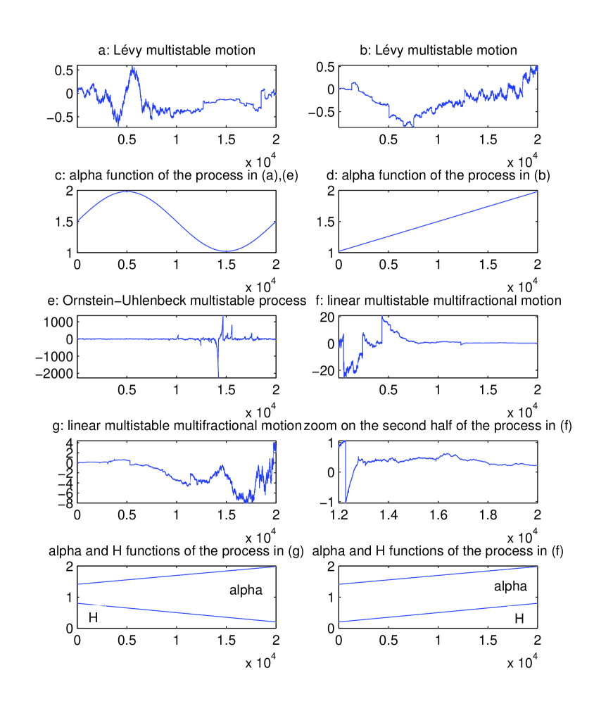
Figure 1: Paths of multistable processes. First line: Levy multistable motions with sine (a) and linear (b) $\alpha$ function. Second line: (c) $\alpha$ function for the process in (a), (d) $\alpha$ function for the process in (b). Third line: (e) multistable Ornstein-Uhlenbeck process with $\alpha$ function displayed in (c), and (f) linear multistable multifractional motion with linear increasing $\alpha$ and $H$ functions. Fourth line: (g) linear multistable multifractional motion with linear increasing $\alpha$ function and linear decreasing $H$ function, and zoom on the second part of the process in (f). Last line: $\alpha$ and $H$ functions for the process in (g) (left), $\alpha$ and $H$ functions for the process in (f) (right).