Multicommodity flow in Polynomial time

Abstract

The multicommodity flow problem is NP-hard already for two commodities over bipartite graphs. Nonetheless, using our recent theory of $n$-fold integer programming and extensions developed herein, we are able to establish the surprising polynomial time solvability of the problem in two broad situations.

1 Introduction

The multicommodity transshipment problem is a very general flow problem which seeks minimum cost routing of several discrete commodities over a digraph subject to vertex demand and edge capacity constraints. The data for the problem is as follows (see Figure 1 below for a small example).

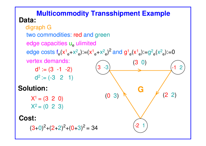
Figure 1: Multicommodity Transshipment Example

There is a digraph $G$ with $s$ vertices and $t$ edges. There are $l$ types of commodities. Each commodity has a demand vector $d^{k}\in\mathbb{Z}^{s}$ with $d^{k}_{v}$ the demand for commodity $k$ at vertex $v$ (interpreted as supply when positive and consumption when negative). Each edge $e$ has a capacity $u_{e}$ (upper bound on the combined flow of all commodities on it). A multicommodity transshipment is a vector $x=(x^{1},\dots,x^{l})$ with $x^{k}\in\mathbb{Z}_{+}^{t}$ for all $k$ and $x^{k}_{e}$ the flow of commodity $k$ on edge $e$, satisfying the capacity constraint $\sum_{k=1}^{l}x^{k}_{e}\leq u_{e}$ for each edge $e$ and demand constraint $\sum_{e\in\delta^{+}(v)}x^{k}_{e}-\sum_{e\in\delta^{-}(v)}x^{k}_{e}=d^{k}_{v}$ for each vertex $v$ and commodity $k$ (with $\delta^{+}(v),\delta^{-}(v)$ the sets of edges entering and leaving vertex $v$).

The cost of transshipment $x$ is defined as follows. There are cost functions $f_{e},g^{k}_{e}:\mathbb{Z}\rightarrow\mathbb{Z}$ for each edge and each edge-commodity pair. The transshipment cost on edge $e$ is $f_{e}(\sum_{k=1}^{l}x^{k}_{e})+\sum_{k=1}^{l}g^{k}_{e}(x^{k}_{e})$ with the first term being the value of $f_{e}$ on the combined flow of all commodities on $e$ and the second term being the sum of costs that depend on both the edge and the commodity. The total cost is

$$\sum_{e=1}^{t}\left(f_{e}\left(\sum_{k=1}^{l}x^{k}_{e}\right)+\sum_{k=1}^{l}g^{k}_{e}(x^{k}_{e})\right)\ .$$

Our results apply to cost functions which can be standard linear or convex such as $\alpha_{e}|\sum_{k=1}^{l}x^{k}_{e}|^{\beta_{e}}+\sum_{k=1}^{l}\gamma^{k}_{e}|x^{k}_{e}|^{\delta^{k}_{e}}$ for some nonnegative integers $\alpha_{e},\beta_{e},\gamma^{k}_{e},\delta^{k}_{e}$, which take into account the increase in cost due to channel congestion when subject to heavy traffic or communication load (with the linear case obtained by $\beta_{e}=\delta^{k}_{e}$=1).

The problem is generally hard: even deciding if a feasible transshipment exists (regardless of its cost) is NP-complete already in the following two very special cases: first, with only $l=2$ commodities over the complete bipartite digraphs $K_{m,n}$ (oriented from one side to the other) [4, 5]; and second, with variable number of commodities over the digraphs $K_{3,n}$ with $m=3$ vertices on one side (see Section 4).

Nonetheless, using the theory of $n$-fold integer programming recently introduced in [2, 3, 9] and extensions developed herein, we are able to establish the surprising polynomial time solvability of the problem, with either standard linear costs or more general costs with nonlinear convex functions $f_{e}$, $g^{k}_{e}$, in two situations as follows.

First, over any fixed digraph, we can solve the problem with a variable number $l$ of commodities (hence termed the many-commodity transshipment problem). This problem may seem at a first glance very restricted: however, even for the single tiny bipartite digraph $K_{3,3}$, we are not aware as of yet of any solution method other than the one provided herein; and as noted, the problem is NP-hard for the digraphs $K_{3,n}$. Our first theorem is the following (see Section 3 for the precise statement).

Theorem 1.1

For any fixed digraph $G$, the (convex) many-commodity transshipment problem with variable $l$ commodities over $G$ can be solved in polynomial time.

We also point out the following immediate corollary of Theorem 1.1.

Corollary 1.2

For any fixed $s$, the (convex) many-commodity transshipment problem with variable $l$ commodities on any $s$-vertex digraph is polynomial time solvable.

The complexity of the algorithm of Theorem 1.1 involves a term of $O\left(l^{g(G)}\right)$ where $g(G)$ is the Graver complexity of $G$, a fascinating new digraph invariant about which very little is known (even $g(K_{3,4})$ is as yet unknown), see discussion in Section 4.

Second, when the number $l$ of commodities is fixed, we can solve the problem over any bipartite subdigraph of $K_{m,n}$ (the so-called multicommodity transportation problem) with fixed number $m$ of suppliers and variable number $n$ of consumers. This is very natural in operations research applications where few facilities serve many customers. Here each commodity type $k$ may have its own volume $v_{k}$ per unit. Note again that if $l$ is variable then the problem is NP-hard already for $m=3$, so our following second theorem is best possible (see Section 3 for the precise statement).

Theorem 1.3

For fixed $l$ commodities and $m$ suppliers, the (convex) multicommodity transportation problem with variable $n$ consumers is polynomial time solvable.

We point out that the running time of our algorithms depends naturally on the binary-encoding length $\langle d^{k}_{v},u_{e}\rangle$ of the numerical part of the data consisting of the demands and capacities (see Section 3), so our algorithms can handle very large numbers. To get such polynomial running time even in the much more limited situation when both the digraph and the number of commodities are fixed (where the number $lt$ of variables becomes fixed) and where the cost functions are linear, one needs off-hand the algorithm of integer programming in fixed dimension [11]. However, Theorems 1.1 and 1.3 involve variable dimension and [11] does not apply.

In Section 2 we review the recent theory of $n$-fold integer programming and establish a new theorem enabling the solvability of a generalized class of $n$-fold integer programs. In Section 3 we use the results of Section 2 to obtain our multicommodity flow Theorems 1.1 and 1.3. We conclude in Section 4 with a short discussion.

2 $N$-fold integer programming

2.1 Background

Linear integer programming is the following fundamental optimization problem,

$$\min\,\left\{wx\ :\ x\in\mathbb{Z}^{n}\,,\ Ax=b\,,\ l\leq x\leq u\right\}\ ,$$

where $A$ is an integer $m\times n$ matrix, $b\in\mathbb{Z}^{m}$, and $l,u\in\mathbb{Z}_{\infty}^{n}$ with $\mathbb{Z}_{\infty}:=\mathbb{Z}\uplus\{\pm\infty\}$. It is generally NP-hard, but polynomial time solvable in two fundamental situations: the dimension is fixed [11]; the underlying matrix is totally unimodular [10].

Recently, in [2], a new fundamental polynomial time solvable situation was discovered. We proceed to describe this class of so-termed $n$-fold integer programs.

An $(r,s)\times t$ bimatrix is a matrix $A$ consisting of two blocks $A_{1}$, $A_{2}$, with $A_{1}$ its $r\times t$ submatrix consisting of the first $r$ rows and $A_{2}$ its $s\times t$ submatrix consisting of the last $s$ rows. The $n$-fold product of $A$ is the following $(r+ns)\times nt$ matrix,

$$A^{(n)}\quad:=\quad\left(\begin{array}[]{cccc}A_{1}&A_{1}&\cdots&A_{1}\\ A_{2}&0&\cdots&0\\ 0&A_{2}&\cdots&0\\ \vdots&\vdots&\ddots&\vdots\\ 0&0&\cdots&A_{2}\\ \end{array}\right)\quad.$$

The following result of [2] asserts that $n$-fold integer programs are efficiently solvable.

Theorem 2.1

[2] For every fixed integer $(r,s)\times t$ bimatrix $A$, there is an algorithm that, given positive integer $n$, $w\in\mathbb{Z}^{nt}$, $b\in\mathbb{Z}^{r+ns}$, and $l,u\in\mathbb{Z}_{\infty}^{nt}$, solves in time which is polynomial in $n$ and in the binary-encoding length $\langle w,b,l,u\rangle$ of the rest of the data, the following so-termed linear $n$-fold integer programming problem,

$$\min\,\left\{wx\ :\ x\in\mathbb{Z}^{nt}\,,\ A^{(n)}x=b\,,\ l\leq x\leq u\right\}\ .$$

Some explanatory notes are in order. First, the dimension of an $n$-fold integer program is $nt$ and is variable. Second, $n$-fold products $A^{(n)}$ are highly non totally unimodular: the $n$-fold product of the simple $(0,1)\times 1$ bimatrix with $A_{1}$ empty and $A_{2}:=2$ satisfies $A^{(n)}=2I_{n}$ and has exponential determinant $2^{n}$. So this is indeed a class of programs which cannot be solved by methods of fixed dimension or totally unimodular matrices. Third, this class of programs turns out to be very natural and has numerous applications, the most generic being to integer optimization over multidimensional tables. In fact it is universal: the results of [5] imply that any integer program is an $n$-fold program over some simple bimatrix $A$, see Section 4.

The above theorem extends to $n$-fold integer programming with nonlinear objective functions as well. The following two results, from [3] and [9] respectively, assert that the maximization and minimization of certain convex functions over $n$-fold integer programs can also be done in polynomial time. The function $f$ is presented by a comparison oracle that for any two vectors $x,y$ can check if $f(x)\leq f(y)$.

Theorem 2.2

[3] For every fixed $d$ and $(r,s)\times t$ integer bimatrix $A$, there is an algorithm that, given $n$, bounds $l,u\in\mathbb{Z}_{\infty}^{nt}$, integer $d\times{nt}$ matrix $W$, $b\in\mathbb{Z}^{r+ns}$, and convex function $f:\mathbb{Z}^{d}\rightarrow\mathbb{R}$ presented by a comparison oracle, solves in time polynomial in $n$ and $\langle l,u,W,b\rangle$, the convex $n$-fold integer maximization problem

$$\max\{f(Wx)\ :\ x\in\mathbb{Z}^{nt}\,,\ A^{(n)}x=b\,,\ l\leq x\leq u\}\ .$$

In the next theorem, $f$ is separable convex, namely $f(x)=\sum_{i}f_{i}(x_{i})$ with each $f_{i}$ univariate convex. The running time depends also on $\log{\hat{f}}$ with ${\hat{f}}$ the maximum value of $|f(x)|$ over the feasible set (${\hat{f}}$ is not needed to be part of the input).

Theorem 2.3

[9] For every fixed integer $(r,s)\times t$ bimatrix $A$, there is an algorithm that, given $n$, lower and upper bounds $l,u\in\mathbb{Z}_{\infty}^{nt}$, $b\in\mathbb{Z}^{r+ns}$, and separable convex function $f:\mathbb{Z}^{nt}\rightarrow\mathbb{Z}$ presented by a comparison oracle, solves in time which is polynomial in $n$ and $\langle l,u,b,{\hat{f}}\rangle$ the convex $n$-fold integer minimization problem

$$\min\left\{f(x)\ :\ x\in\mathbb{Z}^{nt}\,,\ A^{(n)}x=b\,,\ l\leq x\leq u\right\}\ .$$

2.2 Generalization

We now provide a broad generalization of Theorem 2.3 which will be useful for the multicommodity flow applications to follow and is interesting on its own right.

We need to review some material from [2, 9]. We make use of a partial order $\sqsubseteq$ on $\mathbb{R}^{n}$ defined as follows. For two vectors $x,y\in\mathbb{R}^{n}$ we write $x\sqsubseteq y$ if $x_{i}y_{i}\geq 0$ and $|x_{i}|\leq|y_{i}|$ for $i=1,\ldots,n$, that is, $x$ and $y$ lie in the same orthant of $\mathbb{R}^{n}$ and each component of $x$ is bounded by the corresponding component of $y$ in absolute value. A classical lemma of Gordan [7] implies that every subset of $\mathbb{Z}^{n}$ has finitely-many $\sqsubseteq$-minimal elements. The following fundamental object was introduced in [8].

Definition 2.4

The Graver basis of an integer matrix $A$ is defined to be the finite set ${\cal G}(A)\subset\mathbb{Z}^{n}$ of $\sqsubseteq$-minimal elements in $\{x\in\mathbb{Z}^{n}\,:\,Ax=0,\ x\neq 0\}$.

The Graver basis is typically exponential and cannot be written down, let alone computed, in polynomial time. However, we have the following lemma from [2].

Lemma 2.5

For every fixed integer bimatrix $A$ there is an algorithm that, given $n$, obtains the Graver basis ${\cal G}(A^{(n)})$ of the $n$-fold product of $A$ in time polynomial in $n$.

We also need the following lemma from [9] showing the usefulness of Graver bases.

Lemma 2.6

There is an algorithm that, given an integer $m\times n$ matrix $A$, its Graver basis ${\cal G}(A)$, $l,u\in\mathbb{Z}_{\infty}^{n}$, $b\in\mathbb{Z}^{m}$, and separable convex function $f:\mathbb{Z}^{n}\rightarrow\mathbb{Z}$ presented by a comparison oracle, solves in time polynomial in $\langle A,{\cal G}(A),l,u,b,{\hat{f}}\rangle$, the program

$$\min\{f(x)\ :\ x\in\mathbb{Z}^{n}\,,\ Ax=b\,,\ l\leq x\leq u\}\ .$$

Note that Lemmas 2.5 and 2.6 together imply at once Theorem 2.3 mentioned above.

We proceed with two new lemmas needed in the proof of our generalized theorem.

Lemma 2.7

For every fixed integer $(r,s)\times t$ bimatrix $A$ and $(p,q)\times t$ bimatrix $W$, there is an algorithm that, given any positive integer $n$, computes in time polynomial in $n$, the Graver basis ${\cal G}(B)$ of the following $(r+ns+p+nq)\times(nt+p+nq)$ matrix,

$$B\ :=\ \left(\begin{array}[]{cc}A^{(n)}&0\\ W^{(n)}&I\\ \end{array}\right)\ .$$

Proof. Let $D$ be the $(r+p,s+q)\times(t+p+q)$ bimatrix whose blocks are defined by

$$D_{1}\ :=\ \left(\begin{array}[]{ccc}A_{1}&0&0\\ W_{1}&I_{p}&0\\ \end{array}\right)\ ,\quad D_{2}\ :=\ \left(\begin{array}[]{ccc}A_{2}&0&0\\ W_{2}&0&I_{q}\\ \end{array}\right)\quad.$$

Apply the algorithm of Lemma 2.5 and compute in polynomial time the Graver basis ${\cal G}(D^{(n)})$ of the $n$-fold product of $D$, which is the following matrix:

$$D^{(n)}\ =\ {\small\left(\begin{array}[]{ccc|ccc|c|ccc}A_{1}&0&0&A_{1}&0&0&\cdots&A_{1}&0&0\\ W_{1}&I_{p}&0&W_{1}&I_{p}&0&\cdots&W_{1}&I_{p}&0\\ \hline\cr A_{2}&0&0&0&0&0&\cdots&0&0&0\\ W_{2}&0&I_{q}&0&0&0&\cdots&0&0&0\\ \hline\cr 0&0&0&A_{2}&0&0&\cdots&0&0&0\\ 0&0&0&W_{2}&0&I_{q}&\cdots&0&0&0\\ \hline\cr\vdots&\vdots&\vdots&\vdots&\vdots&\vdots&\ddots&\vdots&\vdots&\vdots\\ \hline\cr 0&0&0&0&0&0&\cdots&A_{2}&0&0\\ 0&0&0&0&0&0&\cdots&W_{2}&0&I_{q}\\ \end{array}\right)}\ .$$

Suitable row and column permutations applied to $D^{(n)}$ give the following matrix:

$$C\ :=\ {\small\left(\begin{array}[]{cccc|cccc|cccc}A_{1}&A_{1}&\cdots&A_{1}&0&0&\cdots&0&0&0&\cdots&0\\ A_{2}&0&\cdots&0&0&0&\cdots&0&0&0&\cdots&0\\ 0&A_{2}&\cdots&0&0&0&\cdots&0&0&0&\cdots&0\\ \vdots&\vdots&\ddots&\vdots&\vdots&\vdots&\ddots&\vdots&\vdots&\vdots&\ddots&\vdots\\ 0&0&\cdots&A_{2}&0&0&\cdots&0&0&0&\cdots&0\\ \hline\cr W_{1}&W_{1}&\cdots&W_{1}&I_{p}&I_{p}&\cdots&I_{p}&0&0&\cdots&0\\ W_{2}&0&\cdots&0&0&0&\cdots&0&I_{q}&0&\cdots&0\\ 0&W_{2}&\cdots&0&0&0&\cdots&0&0&I_{q}&\cdots&0\\ \vdots&\vdots&\ddots&\vdots&\vdots&\vdots&\ddots&\vdots&\vdots&\vdots&\ddots&\vdots\\ 0&0&\cdots&W_{2}&0&0&\cdots&0&0&0&\cdots&I_{q}\\ \end{array}\right)}\ .$$

Obtain the Graver basis ${\cal G}(C)$ in polynomial time from ${\cal G}(D^{(n)})$ by permuting the entries of each element of the latter by the permutation of the columns of ${\cal G}(D^{(n)})$ that is used to get $C$ (the permutation of the rows does not affect the Graver basis).

Now, note that the matrix $B$ can be obtained from $C$ by dropping all but the first $p$ columns in the second block. Consider any element in ${\cal G}(C)$, indexed, according to the block structure, as $(x^{1},x^{2},\dots,x^{n},y^{1},y^{2},\dots,y^{n},z^{1},z^{2},\dots,z^{n})$. Clearly, if $y^{k}=0$ for $k=2,\dots,n$ then the restriction $(x^{1},x^{2},\dots,x^{n},y^{1},z^{1},z^{2},\dots,z^{n})$ of this element is in the Graver basis of $B$. On the other hand, if $(x^{1},x^{2},\dots,x^{n},y^{1},z^{1},z^{2},\dots,z^{n})$ is any element in ${\cal G}(B)$ then its extension $(x^{1},x^{2},\dots,x^{n},y^{1},0,\dots,0,z^{1},z^{2},\dots,z^{n})$ is clearly in ${\cal G}(C)$. So the Graver basis of $B$ can be obtained in polynomial time by

$${\cal G}(B)\,:=\,\left\{(x^{1},\dots,x^{n},y^{1},z^{1},\dots,z^{n})\,:\,(x^{1},\dots,x^{n},y^{1},0,\dots,0,z^{1},\dots,z^{n})\in{\cal G}(C)\right\}\,.$$

This completes the proof.        

In the next lemma and theorem, as before, ${\hat{f}}$ and ${\hat{g}}$ denote the maximum values of $|f(Wx)|$ and $|g(x)|$ over the feasible set (${\hat{f}}$, ${\hat{g}}$ do not need to be part of the input).

Lemma 2.8

There is an algorithm that, given an integer $m\times n$ matrix $A$, an integer $d\times n$ matrix $W$, $l,u\in\mathbb{Z}_{\infty}^{n}$, ${\hat{l}},{\hat{u}}\in\mathbb{Z}_{\infty}^{d}$, $b\in\mathbb{Z}^{m}$, the Graver basis ${\cal G}(B)$ of

$$B\ :=\ \left(\begin{array}[]{cc}A&0\\ W&I\\ \end{array}\right)\ ,$$

and separable convex functions $f:\mathbb{Z}^{d}\rightarrow\mathbb{Z}$, $g:\mathbb{Z}^{n}\rightarrow\mathbb{Z}$ presented by comparison oracles, solves in time polynomial in $\langle A,W,{\cal G}(B),l,u,{\hat{l}},{\hat{u}},b,{\hat{f}},{\hat{g}}\rangle$, the program

$$\min\{f(Wx)+g(x)\ :\ x\in\mathbb{Z}^{n}\,,\ Ax=b\,,\ {\hat{l}}\leq Wx\leq{\hat{u}}\,,\ l\leq x\leq u\}\ .$$

Proof. Define $h:\mathbb{Z}^{n+d}\rightarrow\mathbb{Z}$ by $h(x,y):=f(-y)+g(x)$ for all $x\in\mathbb{Z}^{n}$ and $y\in\mathbb{Z}^{d}$. Clearly, $h$ is separable convex since $f,g$ are. Now, our problem can be rewritten as

$$\min\{h(x,y):(x,y)\in\mathbb{Z}^{n+d},\ \left(\begin{array}[]{cc}A&0\\ W&I\\ \end{array}\right)\left(\begin{array}[]{c}x\\ y\\ \end{array}\right)=\left(\begin{array}[]{c}b\\ 0\\ \end{array}\right),\ l\leq x\leq u,-{\hat{u}}\leq y\leq-{\hat{l}}\}\ ,$$

and the statement follows at once by applying Lemma 2.6 to this problem.        

We can now provide our new theorem on generalized $n$-fold integer programming.

Theorem 2.9

For every fixed integer $(r,s)\times t$ bimatrix $A$ and integer $(p,q)\times t$ bimatrix $W$, there is an algorithm that, given $n$, $l,u\in\mathbb{Z}_{\infty}^{nt}$, ${\hat{l}},{\hat{u}}\in\mathbb{Z}_{\infty}^{p+nq}$, $b\in\mathbb{Z}^{r+ns}$, and separable convex functions $f:\mathbb{Z}^{p+nq}\rightarrow\mathbb{Z}$, $g:\mathbb{Z}^{nt}\rightarrow\mathbb{Z}$ presented by comparison oracles, solves in time polynomial in $n$ and $\langle l,u,{\hat{l}},{\hat{u}},b,{\hat{f}},{\hat{g}}\rangle$, the generalized problem

$$\min\left\{f(W^{(n)}x)+g(x)\ :\ x\in\mathbb{Z}^{nt}\,,\ A^{(n)}x=b\,,\ {\hat{l}}\leq W^{(n)}x\leq{\hat{u}}\,,\ l\leq x\leq u\right\}\ .$$

Proof. First use the algorithm of Lemma 2.7 to compute the Graver basis ${\cal G}(B)$ of

$$B\ :=\ \left(\begin{array}[]{cc}A^{(n)}&0\\ W^{(n)}&I\\ \end{array}\right)\ .$$

Now use the algorithm of Lemma 2.8 to solve the problem in polynomial time.        

3 Multicommodity flows

3.1 Many-commodity transshipment

We begin with our theorem on nonlinear many-commodity transshipment. As in the previous section, ${\hat{f}}$, ${\hat{g}}$ denote the maximum absolute values of the objective functions $f$, $g$ over the feasible set. It is usually easy to determine an upper bound on these values from the problem data (for instance, in the special case of linear cost functions $f$, $g$, bounds which are polynomial in the binary-encoding length of the costs $\alpha_{e}$, $\gamma^{k}_{e}$, capacities $u$, and demands $d^{k}_{v}$, readily follow from Cramer’s rule).

Theorem 1.1 For every fixed digraph $G$ there is an algorithm that, given $l$ commodity types, demand $d^{k}_{v}\in\mathbb{Z}$ for each commodity $k$ and vertex $v$, edge capacities $u_{e}\in\mathbb{Z}_{+}$, and convex costs $f_{e},g^{k}_{e}:\mathbb{Z}\rightarrow\mathbb{Z}$ presented by comparison oracles, solves in time polynomial in $l$ and $\langle d^{k}_{v},u_{e},{\hat{f}},{\hat{g}}\rangle$, the many-commodity transshipment problem,

$$\min \sum_{e}\left(f_{e}\left(\sum_{k=1}^{l}x^{k}_{e}\right)+\sum_{k=1}^{l}g^{k}_{e}(x^{k}_{e})\right)$$

s.t. $$x^{k}_{e}\in\mathbb{Z}\,,\ \ \sum_{e\in\delta^{+}(v)}x^{k}_{e}-\sum_{e\in\delta^{-}(v)}x^{k}_{e}=d^{k}_{v}\,,\ \ \sum_{k=1}^{l}x^{k}_{e}\leq u_{e}\,,\ \ x^{k}_{e}\geq 0\ \ .$$

Proof. Assume $G$ has $s$ vertices and $t$ edges and let $D$ be its $s\times t$ vertex-edge incidence matrix. Let $f:\mathbb{Z}^{t}\rightarrow\mathbb{Z}$ and $g:\mathbb{Z}^{lt}\rightarrow\mathbb{Z}$ be the separable convex functions defined by $f(y):=\sum_{e=1}^{t}f_{e}(y_{e})$ with $y_{e}:=\sum_{k=1}^{l}x^{k}_{e}$ and $g(x):=\sum_{e=1}^{t}\sum_{k=1}^{l}g^{k}_{e}(x^{k}_{e})$. Let $x=(x^{1},\dots,x^{l})$ be the vector of variables with $x^{k}\in\mathbb{Z}^{t}$ the flow of commodity $k$ for each $k$. Then the problem can be rewritten in vector form as

$$\min\left\{f\left(\sum_{k=1}^{l}x^{k}\right)+g\left(x\right)\ :\ x\in\mathbb{Z}^{lt}\,,\ Dx^{k}=d^{k}\,,\ \sum_{k=1}^{l}x^{k}\leq u\,,\ x\geq 0\right\}\ .$$

We can now proceed in two ways.

First way: extend the vector of variables to $x=(x^{0},x^{1},\dots,x^{l})$ with $x^{0}\in\mathbb{Z}^{t}$ representing an additional slack commodity. Then the capacity constraints become $\sum_{k=0}^{l}x^{k}=u$ and the cost function becomes $f(u-x_{0})+g(x^{1},\dots,x^{l})$ which is also separable convex. Now let $A$ be the $(t,s)\times t$ bimatrix with first block $A_{1}:=I_{t}$ the $t\times t$ identity matrix and second block $A_{2}:=D$. Let $d^{0}:=Du-\sum_{k=1}^{l}d^{k}$ and let $b:=(u,d^{0},d^{1},\dots,d^{l}$). Then the problem becomes the $(l+1)$-fold integer program

$$\min\left\{f\left(u-x^{0}\right)+g\left(x^{1},\dots,x^{l}\right)\ :\ x\in\mathbb{Z}^{(l+1)t}\,,\ A^{(l)}x=b\,,\ x\geq 0\right\}\ .$$

By Theorem 2.3 this program can be solved in polynomial time as claimed.

Second way: let $A$ be the $(0,s)\times t$ bimatrix with first block $A_{1}$ empty and second block $A_{2}:=D$. Let $W$ be the $(t,0)\times t$ bimatrix with first block $W_{1}:=I_{t}$ the $t\times t$ identity matrix and second block $W_{2}$ empty. Let $b:=(d^{1},\dots,d^{l})$. Then the problem is precisely the following $l$-fold integer program,

$$\min\left\{f\left(W^{(l)}x\right)+g\left(x\right)\ :\ x\in\mathbb{Z}^{lt}\,,\ A^{(l)}x=b\,,\ W^{(l)}x\leq u\,,\ x\geq 0\right\}\ .$$

By Theorem 2.9 this program can be solved in polynomial time as claimed.        

3.2 Multicommodity transportation

We proceed with our theorem on nonlinear multicommodity transportation. The underlying digraph is $K_{m,n}$ (with edges oriented from suppliers to consumers). The problem over any subdigraph $G$ of $K_{m,n}$ reduces to that over $K_{m,n}$ by simply forcing $0$ capacity on all edges not present in $G$. Note that Theorem 1.1 implies that if $m,n$ are fixed then the problem can be solved in polynomial time for variable number $l$ of commodities. However, we now want to allow the number $n$ of consumers to vary and fix the number $l$ of commodities instead. This seems to be a harder problem (with no seeming analog for non bipartite digraphs), and the formulation below is more delicate. Therefore it is convenient to change the labeling of the data a little bit as follows (see Figure 2 below).

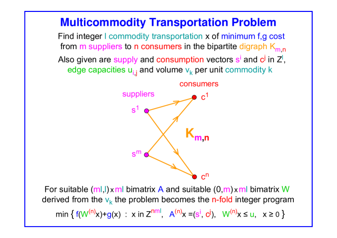
Figure 2: Multicommodity Transportation Problem

We now denote edges by pairs $(i,j)$ where $1\leq i\leq m$ is a supplier and $1\leq j\leq n$ is a consumer. The demand vectors are now replaced by (nonnegative) supply and consumption vectors: each supplier $i$ has a supply vector $s^{i}\in\mathbb{Z}_{+}^{l}$ with $s^{i}_{k}$ its supply in commodity $k$, and each consumer $j$ has a consumption vector $c^{j}\in\mathbb{Z}_{+}^{l}$ with $c^{j}_{k}$ its consumption in commodity $k$. In addition, each commodity $k$ may have its own volume $v_{k}\in\mathbb{Z}_{+}$ per unit flow. A multicommodity transportation is now indexed as $x=(x^{1},\dots,x^{n})$ with $x^{j}=(x^{j}_{1,1},\dots,x^{j}_{1,l},\dots,x^{j}_{m,1},\dots,x^{j}_{m,l})$, where $x^{j}_{i,k}$ is the flow of commodity $k$ from supplier $i$ to consumer $j$. The capacity constraint on edge $(i,j)$ is $\sum_{k=1}^{l}v_{k}x^{j}_{i,k}\leq u_{i,j}$ and the cost is $f_{i,j}\left(\sum_{k=1}^{l}v_{k}x^{j}_{i,k}\right)+\sum_{k=1}^{l}g^{j}_{i,k}\left(x^{j}_{i,k}\right)$ with $f_{i,j},g^{j}_{i,k}:\mathbb{Z}\rightarrow\mathbb{Z}$ convex. As before, ${\hat{f}}$, ${\hat{g}}$ denote the maximum absolute values of $f$, $g$ over the feasible set.

Theorem 1.3 For any fixed $l$ commodities, $m$ suppliers, and volumes $v_{k}\in\mathbb{Z}_{+}$, there is an algorithm that, given $n$, supplies and demands $s^{i},c^{j}\in\mathbb{Z}_{+}^{l}$, capacities $u_{i,j}\in\mathbb{Z}_{+}$, and convex costs $f_{i,j},g^{j}_{i,k}:\mathbb{Z}\rightarrow\mathbb{Z}$ presented by comparison oracles, solves in time polynomial in $n$ and $\langle s^{i},c^{j},u,{\hat{f}},{\hat{g}}\rangle$, the multicommodity transportation problem,

$$\min \sum_{i,j}\left(f_{i,j}\left(\sum_{k}v_{k}x^{j}_{i,k}\right)+\sum_{k=1}^{l}g^{j}_{i,k}\left(x^{j}_{i,k}\right)\right)$$

s.t. $$x^{j}_{i,k}\in\mathbb{Z}\,,\ \ \sum_{j}x^{j}_{i,k}=s^{i}_{k}\,,\ \ \sum_{i}x^{j}_{i,k}=c^{j}_{k}\,,\ \ \sum_{k=1}^{l}v_{k}x^{j}_{i,k}\leq u_{i,j}\,,\ \ x^{j}_{i,k}\geq 0\ \ .$$

Proof. Construct bimatrices $A$ and $W$ as follows. Let $D$ be the $(l,0)\times l$ bimatrix with first block $D_{1}:=I_{l}$ and second block $D_{2}$ empty. Let $V$ be the $(0,1)\times l$ bimatrix with first block $V_{1}$ empty and second block $V_{2}:=(v_{1},\dots,v_{l})$. Let $A$ be the $(ml,l)\times ml$ bimatrix with first block $A_{1}:=I_{ml}$ and second block $A_{2}:=D^{(m)}$. Let $W$ be the $(0,m)\times ml$ bimatrix with first block $W_{1}$ empty and second block $W_{2}:=V^{(m)}$. Let $b$ be the $(ml+nl)$-vector $b:=(s^{1},\dots,s^{m},c^{1},\dots,c^{n})$.

Let $f:\mathbb{Z}^{nm}\rightarrow\mathbb{Z}$ and $g:\mathbb{Z}^{nml}\rightarrow\mathbb{Z}$ be the separable convex functions defined by $f(y):=\sum_{i,j}f_{i,j}(y_{i,j})$ with $y_{i,j}:=\sum_{k=1}^{l}v_{k}x^{j}_{i,k}$ and $g(x):=\sum_{i,j}\sum_{k=1}^{l}g^{j}_{i,k}(x^{j}_{i,k})$.

Now note that $A^{(n)}x$ is an $(ml+nl)$-vector, whose first $ml$ entries are the flows from each supplier of each commodity to all consumers, and whose last $nl$ entries are the flows to each consumer of each commodity from all suppliers. Therefore the supply and consumption equations are encoded by $A^{(n)}x=b$. Next note that the $nm$-vector $y=(y_{1,1},\dots,y_{m,1},\dots,y_{1,n},\dots,y_{m,n})$ satisfies $y=W^{(n)}x$. So the capacity constraints become $W^{(n)}x\leq u$ and the cost function becomes $f(W^{(n)}x)+g(x)$. Therefore, the problem is precisely the following $n$-fold integer program,

$$\min\left\{f\left(W^{(n)}x\right)+g\left(x\right)\ :\ x\in\mathbb{Z}^{nml}\,,\ A^{(n)}x=b\,,\ W^{(n)}x\leq u\,,\ x\geq 0\right\}\ .$$

By Theorem 2.9 this program can be solved in polynomial time as claimed.        

4 Discussion

We conclude with a short discussion of the universality for integer programming of the many-commodity transportation problem and the complexity of our algorithms.

Consider the following special form of the $n$-fold product. For an integer $s\times t$ matrix $D$, let $D^{[n]}:=A^{(n)}$ where $A$ is the $(t,s)\times t$ bimatrix $A$ with first block $A_{1}:=I_{t}$ the $t\times t$ identity matrix and second block $A_{2}:=D$. We consider such $n$-fold products of the $1\times 3$ matrix ${\bf 1}_{3}:=[1,1,1]$. Note that ${\bf 1}_{3}^{[n]}$ is precisely the $(3+n)\times 3n$ incidence matrix of the complete bipartite graph $K_{3,n}$. For instance,

$${\bf 1}_{3}^{[3]}\ =\ \left(\begin{array}[]{ccccccccc}1&0&0&1&0&0&1&0&0\\ 0&1&0&0&1&0&0&1&0\\ 0&0&1&0&0&1&0&0&1\\ 1&1&1&0&0&0&0&0&0\\ 0&0&0&1&1&1&0&0&0\\ 0&0&0&0&0&0&1&1&1\\ \end{array}\right)\ .$$

The following surprising theorem was proved in [5] building on results of [4]. (For further details and consequences for privacy in statistical databases see [5, 6, 12].)

The Universality Theorem [5] Every rational polytope $\{x\in\mathbb{R}_{+}^{d}\,:\,Bx=b\}$ stands in polynomial time computable integer preserving bijection with some polytope

$$\left\{x\in\mathbb{R}_{+}^{3nl}\ :\ {\bf 1}_{3}^{[n][l]}x=a\right\}\ .$$ (1)

In particular, every integer program can be lifted in polynomial time to a program over a matrix ${\bf 1}_{3}^{[n][l]}$ which is completely determined by two parameters $n$ and $l$ only.

Now note (see proof of Theorem 1.1) that the integer points in (1) are precisely the feasible points of some $(l-1)$-commodity transshipment problem over $K_{3,n}$. So every integer program can be lifted in polynomial time to some $l$-commodity program over some $K_{3,n}$. Thus, the many-commodity transportation problem, already over the digraphs $K_{3,n}$ with fixed number $3$ of suppliers, is universal for integer programming. So, in particular, the $l$-commodity transportation problem over $K_{3,n}$ is NP-hard when both $n,l$ are variable, but polynomial time solvable for arbitrary fixed number $n$ of consumers and variable number $l$ of commodities by Theorem 1.1.

Our algorithms involve two major tasks: the construction of the Graver basis of a suitable $n$-fold product in Lemmas 2.5 and 2.7, and the iterative use of this Graver basis to solve the underlying (convex) integer program in Lemmas 2.6 and 2.8. The polynomial time solvability of these tasks is established in [2, 9]. Here we only briefly discuss the complexity of the first task in the special case of a digraph, which is relevant for the complexity of the many-commodity transshipment application.

Let $D$ be the $s\times t$ incidence matrix of a digraph $G$. Consider $l$-fold products $D^{[l]}$ of the special form defined above. The type of an element $x=(x^{1},\dots,x^{l})$ in the Graver basis ${\cal G}(D^{[l]})$ is the number of nonzero blocks $x^{k}\in\mathbb{Z}^{t}$ of $x$. It turns out that for any digraph $G$ there is a finite nonnegative integer $g(G)$ which is the largest type of any element of any ${\cal G}(D^{[l]})$ independent of $l$. We call this new digraph invariant $g(G)$ the Graver complexity of $G$. The complexity of computing ${\cal G}(D^{[l]})$ is $O(l^{g(G)})$ (see [2]) and hence the importance of $g(G)$. Unfortunately, our present understanding of the Graver complexity of a digraph is very limited and much more study is required. Very little is known even for the complete bipartite digraphs $K_{3,n}$ (oriented from one side to the other): while $g(K_{3,3})=9$, already $g(K_{3,4})$ is unknown. See [1] for more details and a lower bound on $g(K_{3,n})$ which is exponential in $n$.

Raymond Hemmecke
Otto-von-Guericke Universität Magdeburg, D-39106 Magdeburg, Germany
email: hemmecke@imo.math.uni-magdeburg.de
  http://www.math.uni-magdeburg.de/$\sim$hemmecke

Shmuel Onn
Technion - Israel Institute of Technology, 32000 Haifa, Israel
and
ETH Zürich, 8092 Zürich, Switzerland
email: onn@ie.technion.ac.il
http://ie.technion.ac.il/$\sim$onn

Robert Weismantel
Otto-von-Guericke Universität Magdeburg, D-39106 Magdeburg, Germany
email: weismantel@imo.math.uni-magdeburg.de
http://www.math.uni-magdeburg.de/$\sim$weismant

References

• [1] Berstein, Y., Onn, S.: The Graver complexity of integer programming. Annals Combin. To appear
• [2] De Loera, J., Hemmecke, R., Onn, S., Weismantel, R.: N-fold integer programming. Disc. Optim. 5 (Volume in memory of George B. Dantzig) (2008) 231–241
• [3] De Loera, J., Hemmecke, R., Onn, S., Rothblum, U.G., Weismantel, R.: Convex integer maximization via Graver bases. J. Pure App. Algeb. 213 (2009) 1569–1577
• [4] De Loera, J., Onn, S.: The complexity of three-way statistical tables. SIAM J. Comp. 33 (2004) 819–836
• [5] De Loera, J., Onn, S.: All rational polytopes are transportation polytopes and all polytopal integer sets are contingency tables. In: Proc. IPCO 10 – Symp. on Integer Programming and Combinatoral Optimization (Columbia University, New York). Lec. Not. Comp. Sci., Springer 3064 (2004) 338–351
• [6] De Loera, J., Onn, S.: Markov bases of three-way tables are arbitrarily complicated. J. Symb. Comp. 41 (2006) 173–181
• [7] Gordan, P.: Über die Auflösung linearer Gleichungen mit reellen Coefficienten. Math. Annalen 6 (1873) 23–28
• [8] Graver, J.E.: On the foundation of linear and integer programming I. Math. Prog. 9 (1975) 207–226
• [9] Hemmecke, R., Onn, S., Weismantel, R.: A polynomial oracle-time algorithm for convex integer minimization. Math. Prog. To appear
• [10] Hoffman, A.J., Kruskal, J.B.: Integral boundary points of convex polyhedra. In: Linear inequalities and Related Systems, Ann. Math. Stud. 38 223–246, Princeton University Press, Princeton, NJ (1956)
• [11] Lenstra Jr., H.W.: Integer programming with a fixed number of variables. Math. Oper. Res. 8 (1983) 538–548
• [12] Onn, S.: Entry uniqueness in margined tables. In: Proc. PSD 2006 – Symp. on Privacy in Statistical Databses (Rome, Italy). Lec. Not. Comp. Sci., Springer 4302 (2006) 94–101