Generation of a symmetric magnetic field
by thermal convection in a plane rotating layer

Vladislav Zheligovsky

International Institute of Earthquake Prediction Theory
and Mathematical Geophysics
84/32 Profsoyuznaya St., 117997 Moscow, Russian Federation

Observatoire de la Côte d’Azur, CNRS
U.M.R. 6529, BP 4229, 06304 Nice Cedex 4, France

We investigate numerically magnetic field generation by thermal convection with square periodicity cells in a rotating horizontal layer of electrically-conducting fluid with stress-free electrically perfectly conducting boundaries for Rayleigh numbers in the interval $5100\leq R\leq 5800$. Dynamos of three kinds, apparently not encountered before, are presented: 1) Steady and time-periodic regimes, where the flow and magnetic field are symmetric about a vertical axis. In regimes with this symmetry, the global $\alpha-$effect is insignificant, and the complex structure of the system of amplitude equations controlling weakly nonlinear stability of the system to perturbations with large spatial and temporal scales suggests that the perturbations are likely to exhibit uncommon complex patterns of behaviour, to be studied in the future work. 2) Periodic in time regimes, where magnetic field is always concentrated in the interior of the convective layer, in contrast to the behaviour first observed by St Pierre (1993) and often perceived as generic for electrically infinitely conducting boundaries. 3) A dynamo exhibiting chaotic behaviour of heteroclinic nature, where a sample trajectory enjoys excursions between a periodic magnetohydrodynamic regime and rolls. The rolls are amagnetic, but generate magnetic field kinematically. As a result, magnetic energy falls off almost to zero, while the rolls are approached.

Keywords: Thermal convection, laminar magnetic dynamo, symmetry about a vertical axis, large-scale stability, heteroclinic cycle.

1 Introduction

Nonlinear regimes of magnetic field generation by Rayleigh-Bénard convection in electrically conducting fluid in a plane layer have not yet been studied in sufficient detail beyond the first bifurcations of the trivial steady state. The only notable exception is the investigation by Podvigina [20, 22], who traced the sequence of bifurcations and attractors for some parameter values on increasing Rayleigh number in the absence of magnetic field, and examined the ability of the convective flows to generate magnetic field in kinematic and nonlinear regimes. A reasonably complete catalogue of convective hydromagnetic (CHM) attractors in various regions of the parameter space, presenting their symmetries and other essential properties, remains so far unavailable. From this prospective, numerous studies performed at present, where MHD or CHM simulations are carried out for extreme parameter values, are of little interest: any emerging structural order in the regimes is ultimately destroyed by chaos in the disguise of turbulence.

The goal of the present study is to look at a series of CHM regimes not far from the onset of convection. We present dynamos of three kinds, to the best of our knowledge not detected before:
$\bullet$ steady and periodic CHM regimes, symmetric about the vertical axis;
$\bullet$ dynamos with magnetic field concentrating in the middle of the layer with perfectly conducting boundaries;
$\bullet$ a chaotic CHM regime where magnetic field occasionally switches off almost entirely.
In the remaining part of the introduction we discuss in what respect in our opinion such dynamos are remarkable.

1.1 The symmetry about a vertical axis and parity invariance

Our main interest lies in convective regimes of magnetic field generation, which are parity-invariant or symmetric about a vertical axis, and stable to perturbations of the same periodicity. Laminar dynamos possessing various symmetries are worth to be identified, for instance, because symmetries play an important rôle in the analysis of dynamical systems and discovery of symmetric regimes can sometimes serve as a basis for a subsequent mathematical investigation providing an insight into different mechanisms of magnetic field generation. In this subsection we discuss the fundamental reasons, coercing us to focus on CHM regimes with the symmetries mentioned in the title. These reasons are related to stability properties of CHM regimes with respect to large-scale perturbations.

Let us remind the definitions of these symmetries. A CHM regime is parity-invariant, if $\bf v$ and $\bf h$ are parity-invariant, and $\theta$ is parity-antiinvariant. A vector field $\bf f$ and a scalar field $f$ are parity-invariant, if

$${\bf f}(-{\bf x},t)=-{\bf f}({\bf x},t);\qquad f(-{\bf x},t)=f({\bf x},t),$$

respectively; they are parity-antiinvariant, if in these equations the signs of the right-hand sides are reversed. (The centre of symmetry must lie on the mid-plane; without any loss of generality we assume that the origin coincides with the centre of symmetry.) A CHM regime is symmetric about the vertical axis, if all the three fields $\bf v$, $\bf h$ and $\theta$ are. A vector field $\bf f$ and a scalar field $f$ are symmetric about a vertical axis, if (again, without any loss of generality assuming that the origin lies on the axis of symmetry)

$$f_{1}(-x_{1},-x_{2},x_{3},t)=-f_{1}(x_{1},x_{2},x_{3},t),$$

$$f_{2}(-x_{1},-x_{2},x_{3},t)=-f_{2}(x_{1},x_{2},x_{3},t),$$

$$f_{3}(-x_{1},-x_{2},x_{3},t)=f_{3}(x_{1},x_{2},x_{3},t),$$

and

$$f(-x_{1},-x_{2},x_{3})=f(x_{1},x_{2},x_{3}),$$

respectively; they are antisymmetric, if in these equations the signs of the right-hand sides are reversed. The two symmetries are compatible with the equations (1)-(4) and with the boundary conditions (5)-(7) considered in the present study (see the next section). For periodic regimes, the symmetries can also involve a time shift by a half of the period.

In this and the following paragraph we summarise the findings of Zheligovsky [30, 31], who considered weakly nonlinear stability of short-scale CHM regimes to large-scale perturbations (involving scales that are much larger than the size of the periodicity cell of the perturbed CHM regime). Generically, large-scale stability is controlled by the (global) combined kinetic and magnetic $\alpha-$effect. Equations governing the evolution of weakly nonlinear large-scale perturbations (more precisely, of the leading terms in expansion in power series in the scale ratio $\varepsilon$ of averaged in small scales amplitudes of neutral small-scale stability modes, comprising the perturbation) are linear; thus, they lack any inherent mechanism for saturation of perturbations. Moreover, they involve no other terms but the slow time derivative and the operator of the combined $\alpha-$effect, and the spectrum of the latter is symmetric about the imaginary axis. Consequently, the equations generically predict a superexponential growth of the perturbations resulting in an ultimate destruction of the perturbed regimes on the time scales O($\varepsilon^{-1}$).

However, if any of the two symmetries under consideration are present, the $\alpha-$effect is insignificant. Apparently (see [3, 5]; note that different quantities are used ibid. and in [30, 31] to measure the strength of the $\alpha-$effect – they are based on the physical common sense in the first case, and ensue from the multiscale asymptotic analysis without a recourse to any empirical relation in the second case), magnetic $\alpha-$effect can also disappear in highly turbulent regimes, but simulations do not demonstrate this conclusively. In the absence of significant combined $\alpha-$effect weakly nonlinear large-scale perturbations are controlled by a system of nonlinear PDE’s for amplitudes of neutral small-scale stability modes. The system is mixed: equations for the mean magnetic field are evolutionary, the rest ones are not; it can involve cubic nonlinearity (see [31]). In contrast to the case of the presence of significant $\alpha-$effect, a priori the equations do not rule out saturation of perturbations at finite energy levels. Instability to large-scale perturbations, if present, develops in MHD systems with such symmetries on much larger time scales, O($\varepsilon^{-2}$). Since in the absence of significant $\alpha-$effect weakly nonlinear large-scale perturbations are controlled by a highly complex system of nonlinear PDE’s, the perturbations are likely to exhibit a variety of uncommon complex patterns of behaviour.

One can look at the same problem at a different angle. Many convective hydrodynamic and hydromagnetic regimes are essentially non-space-periodic. The well-known examples include the Küppers-Lortz [10, 4] and the small-angle (see [21, 23] and references therein) instabilities. Consequently, simulations of convective hydrodynamic and MHD regimes in periodic boxes are not physically sound. Moreover, convection in a horizontally unconstrained domain can “choose” the preferred wave lengths – e.g. on the onset of convective motion the width of convective rolls can be uniquely determined [6]. One may try to overcome this difficulty in computations by largely expanding the box in horizontal directions. The preferred wave lengths of the convective system, which are a priori unknown, are approximated the better, the larger is the box; however, the fundamental deficiency of this approach (followed, for instance, in [3, 5]) – in that the set of wave lengths involved in computations is uniformly discrete – remains invincible. Perhaps, employment of asymptotic multiscale solutions in the style of [9, 30, 31] is at present the only alternative method, not suffering from this inadequacy, although it has its own limitations.

We are hence in need of examples of CHM regimes possessing any of the above mentioned symmetries to carry out, in the future work, case studies of their large-scale perturbations. Podvigina [20, 22] reported instances of hydrodynamic steady and time-periodic convective regimes, that were symmetric about a vertical axis and stable to short-scale perturbations (hence non-chaotic) of the same period, as the perturbed short-scale CHM regime; however, they failed to generate magnetic field with the same symmetry. We have found steady and time-periodic CHM regimes, which are symmetric about a vertical axis.

1.2 Concentration of magnetic field in the middle of a layer
with perfectly conducting boundaries

We study convection in a plane rotating layer with stress-free perfectly conducting boundaries held at constant temperatures. Magnetic field generation by thermal convection with square periodicity cells in the nonlinear regime was explored for these boundary conditions in [14, 25, 11, 7, 26, 3, 5, 20, 22]. Simulations [14, 3, 5] were performed for much higher Rayleigh numbers (of the order of $10^{5}-10^{6}$) than the critical ones, resulting in the onset of a turbulence-like behaviour of solutions. In the remaining studies cited above the Rayleigh number did not exceed a moderate multiple of the critical value and convective flows exhibited laminar behaviour, although instances of chaotic behaviour of MHD systems – precursors to turbulence – were also obtained. The case of fast rotation was considered in [25, 26]; the Rayleigh number was kept below the critical value for the onset of non-magnetic convection in [25]. Magnetic field showed a variety of patterns of behaviour.

In the convective dynamos [25, 11] magnetic field concentrated near the boundaries in sublayers of the width of a quarter of the layer width. Magnetic energy attained the maximum on the boundary in the run labeled N6 in [14] (see a snapshot of magnetic field on fig. 6 ibid.; no detailed information is presented about the spatial distribution of magnetic field in other runs). St Pierre [25] suggested a physical mechanism for explanation of concentration of magnetic field near infinitely electrically conducting boundaries: if the fluid motion in the vertical direction is not inhibited, magnetic field is advected to a boundary and remains “locked” there, unable to exit from the fluid layer outside the boundary acting as a screen. Thus, these boundary conditions can be beneficial for magnetic field generation. (In dynamo simulations [27] in a plane convective layer and [24] in a rotating spherical fluid shell, the efficiency of dynamo was not significantly affected by the boundary conditions for magnetic field, which were varied only on the inner core boundary in [24].) In the convective dynamos [20, 22] in a non-rotating layer, strong magnetic field usually formed ropes near the boundaries, however, Podvigina [22] found chaotic regimes, where magnetic field was residing part of the time near the boundaries and part of the time inside the layer. Magnetic field computed in [7] had a form of cigar-like structures of vertical orientation, mostly located inside the layer, with small blobs of strong field near the horizontal boundaries. In the convective dynamo computations [26] for a much faster than in our simulations rotation, magnetic field was organised into irregular structures with magnetic energy most time residing inside the fluid layer.

We have encountered CHM time-periodic regimes, in which, in contrast with all the simulations mentioned above, the generated magnetic field always remains concentrated in the interior of the convective layer.

1.3 A heteroclinic CHM regime
with occasional disappearance of magnetic field

We have found a chaotic CHM regime of a heteroclinic nature, where a trajectory jumps between a CHM periodic orbit and amagnetic steady rolls. Both, the orbit and the rolls, are slightly unstable. The rolls are capable of kinematic magnetic field generation, however, while the trajectory approaches the rolls after the regime has deviated from the periodic oscillations, magnetic energy decays almost to zero before the growing magnetic mode becomes substantial.

From the viewpoint of the theory of dynamical systems, nothing is particularly surprising in such a behaviour: heteroclinic cycles between a periodic orbit and two steady states were studied in [12] and were observed, for instance, in [13] in a low-order dynamical system, modelling excursions and reversals of the Earth’s magnetic field. To the best of our knowledge, such behaviour was never before found in numerical simulations of “real” physical systems. It is notable, that this CHM regime and regimes observed for some sets of parameter values in the VKS (von Kármán Sodium) experiment [16] exhibit certain similar features, such as intermittency with bursts and extinction of magnetic field (see fig. 25 ibid.) and heteroclinic connections of unstable MHD steady states (but the regimes of heteroclinic nature apparently do not involve connections to periodic orbits).

2 Numerical simulation

Evolution of the Boussinesq CHM system satisfies the non-dimensional Navier-Stokes, magnetic induction and heat transfer equations:

$${\partial{\bf v}\over\partial t}=P\nabla^{2}{\bf v}+{\bf v}\times\mbox{\boldmath$\omega$\unboldmath}-{\bf h}\times(\nabla\times{\bf h})+P\tau{\bf v}\times{\bf e}_{3}+PR\theta{\bf e}_{3}-\nabla p,$$

$${\partial{\bf h}\over\partial t}={P\over P_{m}}\nabla^{2}{\bf h}+\nabla\times({\bf v}\times{\bf h}),$$

$${\partial\theta\over\partial t}=\nabla^{2}\theta-({\bf v}\cdot\nabla)\theta+v_{3},$$

and the solenoidality conditions

$$\nabla\cdot{\bf v}=0,\qquad\nabla\cdot{\bf h}=0.$$

Here $\bf h$ and $\mbox{\boldmath$\omega$\unboldmath}=\nabla\times\bf v$ denote velocity and vorticity, respectively, of a flow of an electrically conducting fluid, $p$ modified pressure, $\bf h$ magnetic field, $\theta=T-(x_{3}+L/2)$ the difference between the normalised temperature $T$ and the linear temperature profile in the layer in the absence of fluid motion; $t$ is time, $P$, $P_{m}$, $R$ and $\tau^{2}$ are kinematic Prandtl, magnetic Prandtl, Rayleigh and Taylor numbers, respectively, $\tau/2$ is the normalised angular rotation rate, ${\bf e}_{k}$ the unit vector along the axis $x_{k}$ of the Cartesian coordinate system co-rotating with the layer; $L$ is the width of the layer. The CHM system is free: no external sources are present in equations (1)-(3). Hence, the regimes are spatially and temporally invariant – there is no explicit dependence of any term in the equations either on the position in space, or on time.

We assume that the horizontal boundaries of the layer are stress-free:

$$\left.{\partial v_{1}\over\partial x_{3}}\right|_{x_{3}=\pm L/2}=\left.{\partial v_{2}\over\partial x_{3}}\right|_{x_{3}=\pm L/2}=0,\quad\left.v_{3}\right|_{x_{3}=\pm L/2}=0,$$

infinitely electrically conducting:

$$\left.{\partial h_{1}\over\partial x_{3}}\right|_{x_{3}=\pm L/2}=\left.{\partial h_{2}\over\partial x_{3}}\right|_{x_{3}=\pm L/2}=0,\quad\left.h_{3}\right|_{x_{3}=\pm L/2}=0,$$

and kept at fixed temperatures:

$$\theta\left|{}_{x_{3}=\pm L/2}=0.\right.$$

These boundary conditions are the most convenient ones for simulation of Boussinesq convection in the layer. They were used in all numerical dynamo simulations cited in the Introduction, (5) was assumed in the investigation [21, 23] (also see references therein) of the hydrodynamic small-angle instability, and stability regimes to large-scale perturbations were studied in [30, 31] also for (5)-(7).

We have carried out a numerical search for examples of symmetric CHM attractors with the same period $L_{h}$ along the horizontal coordinate axes $x_{1}$ and $x_{2}$. To avoid turbulisation of the flow and symmetry breaking, we have not used extreme parameter values like in some studies cited in the Introduction. Simulations have been performed for $L=1$, $L_{h}=10/7$, $P=1$, $\tau=91$ (i.e. the Taylor number is 8281) for $R$ increasing from 5100 to 5800. For these values, the critical Rayleigh number for the onset of convective flow in the absence of magnetic field is equal to $\sim$5514; for the periodicity box, which is $\sqrt{2}$ times smaller in size and aligned with the diagonals of the computational periodicity box, the critical Rayleigh number is $\sim$5072 (the two critical numbers have been evaluated using a precise formula for $R$ derived in [6] for the boundary conditions assumed here).

As discussed in the Introduction, our prime goal is to find symmetric CHM regimes. In the primary (hydrodynamic) bifurcation convective flows in the form of rolls set in, which possess the desirable symmetry. Because of rotation, they can (at least in principle) kinematically generate magnetic field, if magnetic Prandtl number is high enough; if the dominant magnetic mode also has the symmetry, then the CHM regime emerging in the secondary (magnetic) bifurcation remains symmetric. Consequently, we have chosen to perform simulations for a (relatively) high value $P_{m}=100$ (in contrast with $P_{m}<1$ used for numerical simulations of the Earth’s dynamo, characterised by the values $P_{m}\sim 10^{-5}$).

Unlike in [20, 22], we have not attempted to analyse the sequence of occurring bifurcations in detail, or to locate them to a good accuracy, nor to identify all attractors of the CHM system for any considered $R$.

Table. Regimes of thermal hydromagnetic convection. $E^{k}_{\min},\ E^{k}_{\rm av},\ E^{k}_{\max}$: kinetic energy per periodicity cell, minimal, average over a period and maximal, respectively; $E^{m}_{\min},\ E^{m}_{\rm av},\ E^{m}_{\max}$: the same for magnetic energy. SVA: symmetry about the vertical axis ($+$: $\bf v$ and $\bf h$ are both symmetric; $-$: $\bf v$ is symmetric and $\bf h$ is antisymmetric; 0: $\bf v$ is symmetric, no magnetic field generation; No: $\bf v$ and $\bf h$ do not possess the symmetry or antisymmetry). P: parity related symmetries (see the text). Type: the type of regime (SS: a steady state, DR: steady rolls aligned with the diagonal, with $n_{1}\!=\!n_{2}$ and $n_{3}$ of the same parity in (8), HC: heteroclinic chaos, a number: temporal frequency of a periodic orbit).

$R$ $E^{k}_{\min}$ $E^{k}_{\rm av}$ $E^{k}_{\max}$ $E^{m}_{\min}$ $E^{m}_{\rm av}$ $E^{m}_{\max}$ SVA P Type 5100 1.0 1.0 1.0 0.012 0.012 0.012 $+$ $\sigma_{1}$ SS 5140 2.4 2.4 2.4 0.025 0.025 0.025 $+$ $\sigma_{1}$ SS 5160 4.9 5.3 5.8 1.30 1.46 1.71 $-$ 0.18 5180 5.8 6.3 7.0 1.58 1.84 2.28 $-$ 0.19 5190 6.3 6.9 7.7 1.75 2.10 2.68 $-$ 0.19 5210 5.2 6.8 16.1 0.33 1.86 12.8 $-$ HC 5210 6.5 6.5 6.5 0 0 0 0 DR 5220 6.9 6.9 6.9 0 0 0 0 DR 5230 6.7 6.7 6.7 0 0 0 0 DR 5240 7.9 7.9 7.9 0 0 0 0 DR 5250 8.4 8.4 8.4 0 0 0 0 DR 5260 8.8 8.8 8.8 0 0 0 0 DR 5300 10.8 10.8 10.8 0 0 0 0 DR 5350 9.8 10.0 10.4 0.30 0.55 0.95 $+$ $\sigma_{1}$ 0.315 5400 11.5 12.0 13.0 0.26 0.75 1.85 $+$ $\sigma_{1}$ 0.31 5500 15.1 16.0 19.0 0.27 1.13 3.71 $+$ $\sigma_{1}$ 0.32 5550 16.9 18.0 22.9 0.25 1.15 4.68 $+$ $\sigma_{1}$ 0.29 5600 20.3 22.3 25.5 1.56 2.30 3.77 No $\sigma_{2}$ 0.66 5700 24.6 27.3 31.0 2.20 3.20 4.91 $-$ $\sigma_{2}$ 0.76 5750 26.3 29.8 33.9 2.28 3.71 5.62 No $\sigma_{2}$ 0.38 5800 26.1 33.0 39.7 0 3.70 27.12 No $\sigma_{3}$ HC

For the boundary conditions under consideration, the fields are expanded in the Fourier series

$${\bf v}=\sum_{{\bf n}:\ n_{3}\geq 0}\left[\begin{array}[]{c}v_{{\bf n},1}\cos n_{3}\pi(x_{3}/L+1/2)\\ v_{{\bf n},2}\cos n_{3}\pi(x_{3}/L+1/2)\\ v_{{\bf n},3}\sin n_{3}\pi(x_{3}/L+1/2)\end{array}\right]{\rm e}^{{2\pi i\over L_{h}}(n_{1}x_{1}+n_{2}x_{2})},$$

$${\bf h}=\sum_{{\bf n}:\ n_{3}\geq 0}\left[\begin{array}[]{c}h_{{\bf n},1}\cos n_{3}\pi(x_{3}/L+1/2)\\ h_{{\bf n},2}\cos n_{3}\pi(x_{3}/L+1/2)\\ h_{{\bf n},3}\sin n_{3}\pi(x_{3}/L+1/2)\end{array}\right]{\rm e}^{{2\pi i\over L_{h}}(n_{1}x_{1}+n_{2}x_{2})},$$

$$\theta=\sum_{{\bf n}:\ n_{3}>0}\theta_{\bf n}\sin n_{3}\pi(x_{3}/L+1/2)\,{\rm e}^{{2\pi i\over L_{h}}(n_{1}x_{1}+n_{2}x_{2})}.$$

Solenoidality conditions (4) for the series (8) and (9) take the forms

$${2\pi in_{1}\over L_{h}}v_{{\bf n},1}+{2\pi in_{2}\over L_{h}}v_{{\bf n},2}+{\pi n_{3}\over L}v_{{\bf n},3}=0;$$

$${2\pi in_{1}\over L_{h}}h_{{\bf n},1}+{2\pi in_{2}\over L_{h}}h_{{\bf n},2}+{\pi n_{3}\over L}h_{{\bf n},3}=0.$$

Standard pseudospectral methods (see [2, 1, 17]) have been applied with the resolution of $64\times 64\times 32$ Fourier harmonics (after dealiasing in computation of advective terms was performed). The energy spectra of the computed attractors decay by several (at least 3-4 for magnetic field, which has the least decreasing energy spectrum) orders of magnitude. No significant discrepancies with the results of several test runs with the $128\times 128\times 64$ resolution have been found.

3 Results of computation

Properties of the observed CHM attractors are summarised in the table. In the interval $5210\leq R\leq 5300$ they degenerate into a system of two-dimensional rolls aligned with the diagonal of the periodicity box, in which the flow is independent from the position along the axes of the rolls. Although the flows in the rolls has all the three spatial components and the Zeldovich antidynamo theorem [28] is not applicable, the rolls do not generate magnetic field. In all other saturated regimes that have been simulated, generation takes place.

For most attractors found in computations, the sums (8)-(10) turn out to be comprised of terms, where for some $i,j=1,2,3$ the sum $n_{i}+n_{j}$ has a certain parity (see the table). Suppose $v_{{\bf n},i}\neq 0$ only, if $n_{i}+n_{j}$ is even. This is consistent with the action of the Lorentz force (quadratic in $\bf h$) in the Navier-Stokes equation (1) only, if for all non-zero terms in (8) parity of $n_{i}+n_{j}$ is the same – either odd, or even. If a scalar or vector field is represented by a sum of the form of (10) or (8), respectively, where $n_{1}+n_{2}$ is even, then the size of its elementary periodicity cell is $L_{h}/\sqrt{2}$, and the cell sides are oriented along the diagonals of the computational periodicity cell. In particular, for $R=5100$, 5140 and $5350\leq R\leq 5700$ $v_{{\bf n},i}\neq 0$ only, if $n_{1}+n_{2}$ is even, and $h_{{\bf n},i}\neq 0$ only, if $n_{1}+n_{2}$ is odd. Thus, the periodicity cell of the flow is $\sqrt{2}$ times less than the periodicity cell of magnetic field, i.e. a mild scale separation is present in these CHM regimes. If coefficients of a field do not vanish only, if $n_{j}+n_{3}$ is even ($j=1$ or 2), it has a symmetry, which is a composition of translation by a half of period along the axis $x_{j}$ and reflection about the mid-plane. The following three combinations of symmetries of this kind have been encountered in computations:
$\sigma_{1}$: $v_{{\bf n},i}\neq 0$ only, if ${\rm mod}_{2}\,n_{1}={\rm mod}_{2}\,n_{2}={\rm mod}_{2}\,n_{3}$ and $h_{{\bf n},i}\neq 0$ only, if ${\rm mod}_{2}\,n_{1}\neq{\rm mod}_{2}\,n_{2}={\rm mod}_{2}\,n_{3}$;
$\sigma_{2}$: $v_{{\bf n},i}\neq 0$ only, if ${\rm mod}_{2}\,n_{1}={\rm mod}_{2}\,n_{2}={\rm mod}_{2}\,n_{3}$ and $h_{{\bf n},i}\neq 0$ only, if ${\rm mod}_{2}\,n_{1}={\rm mod}_{2}\,n_{2}\neq{\rm mod}_{2}\,n_{3}$;
$\sigma_{3}$: $v_{{\bf n},i}\neq 0$ only, if ${\rm mod}_{2}\,n_{2}={\rm mod}_{2}\,n_{3}$ and $h_{{\bf n},i}\neq 0$ only, if ${\rm mod}_{2}\,n_{2}\neq{\rm mod}_{2}\,n_{3}$. (We use here the standard notation ${\rm mod}_{2}\,n$ for parity of $n$: it is 0 for even $n$, and 1 for odd $n$.)

Except for $R=5600$ and 5800, the flows in attractors are symmetric about the vertical axis (see the table); in agreement with this, magnetic field either has the same symmetry, or it is antisymmetric. All the simulated CHM regimes, in which all the three constituent fields possess this symmetry, exhibit a simple time dependence: they are steady or periodic, and in addition have the symmetries $\sigma_{1}$, in particular, implying scale separation.

         

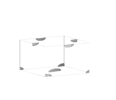
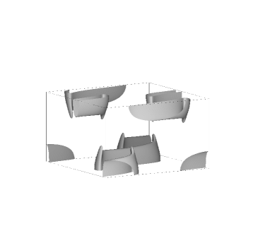
(a)                                                                 (b)

Figure 1: Isosurfaces of magnetic energy density $|{\bf h}|^{2}$ at the levels of 2/3 (a) and 1/20 (b) of the maximum for the CHM steady state for $R=5100$. One periodicity cell is shown.

(a)  

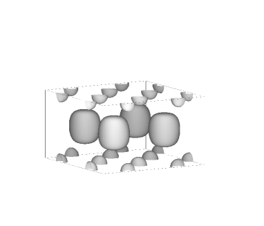
(b)                (c)  

Figure 2: Isosurfaces of kinetic energy density $|{\bf v}|^{2}$ at the level of a half of the maximum (a) and the flow on the mid-plane $x_{3}=0$: horizontal components (b) of the velocity of the fluid and isolines of the vertical component (c) of the velocity step 0.3 (zero and positive values: solid lines, negative values: dashed lines) for the CHM steady state for $R=5100$. One periodicity cell is shown.

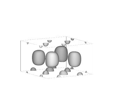
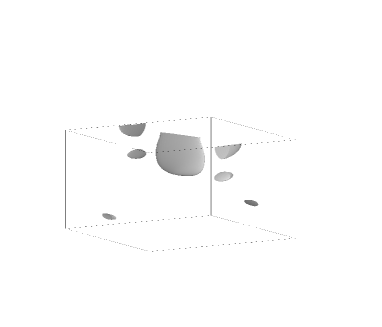
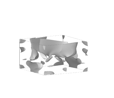
Figure 3: Isosurfaces of kinetic energy density $|{\bf v}|^{2}$ at the level of a half of the maximum for the time-periodic CHM regime for $R=5180$. One periodicity cell at a randomly chosen time is shown.

         

(a)                                                                 (b)

Figure 4: Isosurfaces of magnetic energy density $|{\bf h}|^{2}$ at the levels of 1/2 (a) and 1/10 (b) of the maximum for the time-periodic CHM regime for $R=5180$. One periodicity cell is shown at the time, for which fig. 4 is constructed.

CHM regimes for $5100\leq R\leq 5140$ are steady states (see figs. 2 and 2). As documented in [25], magnetic field generated by convective flows tends to concentrate near infinitely electrically conducting boundaries of the layer. Magnetic flux ropes (fig. 2a) generated by steady flows are associated with stagnation points of the flow, which have one-dimensional unstable and two-dimensional stable manifolds (asymptotic solutions of the magnetic induction equation describing magnetic ropes in the vicinity of such stagnation points were presented in [15, 29, 8]); the ropes are cut in halves along their axes by the boundaries of the layer. In the steady CHM state for $R=5100$, stagnation points of the flow are located on the midplane and on the upper and lower boundaries of the box of periodicity shown on fig. 2. On each of the three horizontal planes they constitute a square mesh of mesh size $L_{h}/\sqrt{8}$, oriented along the diagonals of the periodicity cells. Only stagnation points at the centre and in the vertices of the horizontal faces of the shown box of periodicity are associated with the magnetic flux ropes. The flow can be described as a system of downward and upward swirls (fig. 2) positioned in the chessboard order. Inward flows advect magnetic field from the magnetic ropes near the boundaries towards the middle of the layer with formation of magnetic flux sheets between adjacent swirls (fig. 2b).

Figure 5: Total kinetic (upper curve) and magnetic (lower curve) energies (vertical axis) as a function of time (horizontal axis) for the chaotic CHM regime for $R=5210$.

A branch of periodic orbits exists for $5160\leq R\leq 5190$. (For symmetry reasons, this branch of periodic regimes does not emerge from the branch of steady states.) The symmetry about the vertical axis of the flow and temperature is preserved, but magnetic field is now antisymmetric (and significantly stronger). Unlike for the CHM steady states observed for smaller considered $R$, there is no parity selection of wave numbers in the Fourier series (8)-(10) representing the solutions. However, the structures of the flow and (to a lesser extent) magnetic field resembles those for $R=5100$ (fig. 4, 4a). The main feature of magnetic field is vertical magnetic flux sheets (fig. 4b), resembling sheets developing in the vicinity of an unstable manifold of a stagnation point of the flow, if the point has a two-dimensional unstable and one-dimensional stable manifolds (asymptotic analysis of solutions of the magnetic induction equation in this context was carried out by Childress and Soward 1985).

At $R=5210$ two CHM attractors are found in the system: amagnetic steady rolls and an attractor exhibiting heteroclinic chaotic behaviour (fig. 5). In the phases of oscillations of growing amplitude the system is in the vicinity of the former periodic orbit. The sample trajectory vigorously exponentially departures from it, but subsequently comes to the phase of lower kinetic and magnetic energy levels, during which it is in the vicinity of a mildly unstable steady state, near which integration of the sample trajectory has begun. Duration of this phase can be quite short. The phase of evolution near the steady state also finishes in an exponential departure, with kinetic and magnetic energy surges of amplitude comparable to that of energy surges during departures from the phase of evolution near the periodic orbit. Sample trajectories which start in the vicinity of the same steady state for higher $R$, are attracted to steady rolls in shorter times, than the length of integration of the trajectory for $R=5210$; however, their behaviour at the intermediate transitory stage resembles the chaotic behaviour for $R=5210$, and thus from a conservative point of view it cannot be excluded, that duration of the chaotic stage at $R=5210$ is also finite.

         

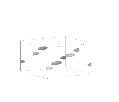
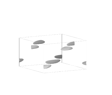
$t=0$                                                              $t=T/8$

         

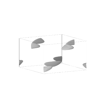
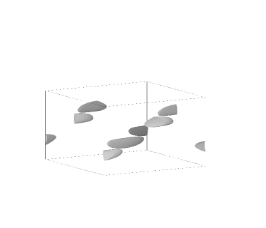
$t=T/4$                                                            $t=3T/8$

         

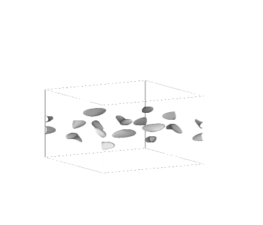
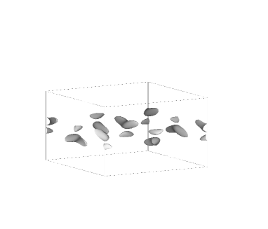
$t=T/2$                                                            $t=5T/8$

Figure 6: Isosurfaces of magnetic energy density $|{\bf h}|^{2}$ at the level of 1/2 of the maximum for the time-periodic CHM regime for $R=5400$. One periodicity cell is shown step 1/8 of the temporal period $T$.

         

$t=3T/4$                                                            $t=7T/8$

Figure 6 (the end)

  

$R=5350$

$R=5400$

  

$R=5500$           $R=5550$

$R=5600$

Figure 7: Distances (vertical axis) from sets, where magnetic energy density is equal to or exceeds $e_{\max}(t)/16$ (thin short-dashed line), $e_{\max}(t)/8$ (dash-and-dots line), $e_{\max}(t)/4$ (dotted line), $e_{\max}(t)/2$ (thin long-dashed line) and ${15\over 16}e_{\max}(t)$ (thin solid line) to the closest boundaries of the fluid layer for $5350\leq R\leq 5600$ as a function of time (horizontal axis). Thick solid line: normalised total magnetic energy $E^{m}(t)/\max_{t}E^{m}(t)$, thick dashed line: normalised total kinetic energy $E^{k}(t)/\max_{t}E^{k}(t)$. One temporal period is shown.

         

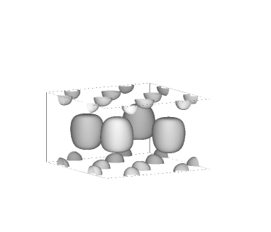
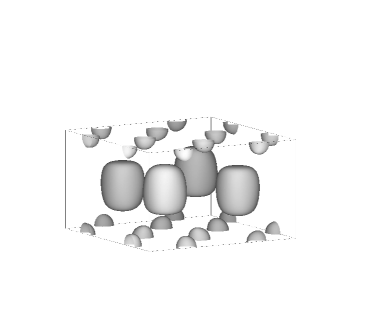
$t=0$                                                            $t=T/2$

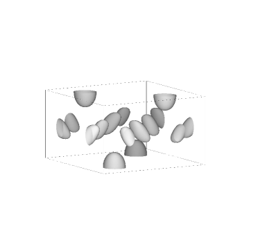
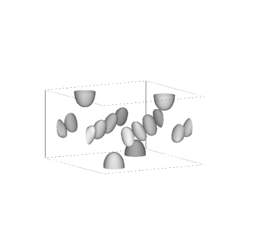
Figure 8: Isosurfaces of kinetic energy density $|{\bf v}|^{2}$ at the level of a half of the maximum for the periodic CHM regime for $R=5400$. One periodicity cell is shown step a half of the temporal period.

         

$t=0$                                                            $t=T/2$

Figure 9: Isosurfaces of vorticity density $|\nabla\times{\bf v}|^{2}$ at the level of 2/3 of the maximum for the periodic CHM regime for $R=5400$. One periodicity cell is shown step a half of the temporal period.

The window of amagnetic convective rolls is followed by a sequence of periodic regimes in the interval $5350\leq R\leq 5550$. Periodic CHM regimes from the branch for $5350\leq R\leq 5550$ exhibit an interesting feature: whilst for $5100\leq R\leq 5190$ the strongest magnetic field is located on boundaries of the convective layer, in the former Rayleigh number interval the maximum of magnetic field density is always ($5350\leq R\leq 5500$) or most of the time ($R=5550$) is in the interior of the layer (see fig. 6, 7; segments of some plots are not visible on fig. 7 for the times, where the distance vanishes). This is in contrast with the behaviour found in all previous computations. For $0\leq s\leq 1$, denote by $U_{s}(t)$ the set of points in the layer, where at time $t$ magnetic energy density $|{\bf h}|^{2}$ is equal to or exceeds the value $se_{\max}(t)$, $e_{\max}(t)$ being the maximum of magnetic energy density spatial distribution at time $t$. For $R=5350$ and 5400, the set $U_{15/16}(t)$ is always at a distance of at least 0.226 and 0.156 of the layer width away from the boundaries, and $U_{1/2}(t)$ is not less than 0.133 and 0.057 of the width away, respectively. Consequently, these CHM regimes may be not very sensitive to the boundary conditions for magnetic field. In all simulated CHM regimes the distance is the smallest (in time) near the points of maxima of the total kinetic and magnetic energies. Concentration of magnetic field in the interior of the layer can be related to the fact, that the regions of the most vigorous flow motions are inside it (fig. 9, 9). Since isosurfaces shown on these figures only weakly depend on time, they are presented step a half of the temporal period, when the difference in their shape is extreme. (Vorticity admits the maximum on the boundaries of the layer; both the flow and vorticity are strong in some regions close to the boundaries, but the size of these regions is comparatively small, which may explain why they do not influence magnetic field generation significantly.)

The branch existing for $5350\leq R\leq 5550$ apparently disappears between $R=5550$ and 5600. For $R=5600$ the regime is a periodic orbit of temporal frequency more than twice higher (see the table). It has a different symmetry group: it is the only periodic orbit that we have found, where the flow is not symmetric about a vertical axis. Between $R=5600$ and 5700 the periodic regime changes once again. At $R=5800$ the CHM regime is a chaotic attractor of heteroclinic nature. Like for $R=5210$, the sample trajectory enjoys excursions between a steady state and a periodic orbit (in this description we do not distinguish states related by discrete symmetries and translation in horizontal directions), but apart from this the patterns of behaviour of the two chaotic attractors are completely different. The periodic orbit emerges from the one for $R=5700$ in a period-doubling bifurcation; in particular, it has all the parity-related symmetries of the latter. This periodic orbit is stable at $R=5750$, but becomes unstable at $R=5800$. The steady state is amagnetic rolls aligned with the diagonal of the periodicity cell and invariant with respect to translations along the axis; therefore, it also possesses all the symmetries of the periodic orbit at $R=5700$. However, all the symmetries are broken during the exponential transition processes when the trajectory moves between the two states, except for the composition of translation in the $x_{2}-$direction and reflection about the mid-plane $\sigma_{3}$. Both states are only marginally unstable. The rolls are apparently capable of kinematic generation of magnetic field, but while the trajectory approaches them, magnetic energy falls off almost to zero (fig. 10).

(a)   

(b)   

Figure 10: Total kinetic (a) and magnetic (b) energies (vertical axes) as functions of time (horizontal axis) for the chaotic CHM regime for $R=5800$. Magnetic energy is shown in logarithmic scale.

4 Conclusion

We have observed a number of steady and periodic CHM attractors, possessing the symmetry about the vertical axis, and several regimes, where this symmetry is broken partially (the magnetic field becoming antisymmetric) or completely. The amplitude equations derived in [31] are applicable for examination of the weakly non-linear stability of the symmetric CHM regimes presented here. It remains to be investigated how disappears the branch of periodic orbits, existing for $5350\leq R\leq 5550$. If this is a symmetry-breaking bifurcation, the system of amplitude equations for free CHM convection, analogous to the system of mean-field equations derived in [30] for a branch of regimes emerging in a Hopf bifurcation in forced CHM convection, might be applicable for examination of weakly nonlinear large-scale stability of the periodic regimes constituting this branch near this bifurcation.

We have found two other types of notable convective magnetic dynamos. One of the regimes is periodic orbits for Rayleigh numbers from the interval $5350\leq R\leq 5500$: it is apparently the first known example of CHM regimes, where the strongest generated magnetic field always resides in the interior of the fluid layer. The second is the heteroclinic chaotic regime for $R=5800$, in which the evolution consists of phases, where the regime is in the vicinity either of a periodic orbit, or a steady state – amagnetic rolls. Dynamics of this attractor can be studied employing expanded central manifold reduction [18, 19].

Acknowledgments

I have benefited from discussions with J.-F. Pinton. Comments of an anonymous Referee have helped to improve the paper. Part of this research was carried out during the visit of the author to the School of Engineering, Computer Science and Mathematics, University of Exeter, UK, in January – April 2008. I am grateful to the Royal Society for their financial support. Computations have been carried out on the computer “Mésocentre SIGAMM (Simulations Interactives et Visualisation en Géophysique, Astronomie, Mathématique et Mécanique)” hosted by Observatoire de la Côte d’Azur, France. My research work at the Observatoire de la Côte d’Azur in the autumns of 2007 and 2008 was supported by the French Ministry of Education. I was partially financed by the grants ANR-07-BLAN-0235 OTARIE from Agence nationale de la recherche, France, and 07-01-92217-CNRSL_a from the Russian foundation for basic research.

References

- [1] J.P. Boyd. Chebyshev and Fourier spectral methods, 2000 (NY: Dover Publ.).
- [2] C. Canuto, M.You. Hussaini, A. Quarteroni, Th.A. Zang. Spectral methods in fluid dynamics, 1988 (Berlin: Springer-Verlag).
- [3] F. Cattaneo, D.W. Hughes. Dynamo action in a rotating convective layer. J. Fluid Mech., 2006, 553, 401-418.
- [4] R.M. Clever, F.H. Busse. Nonlinear properties of convection rolls in a horizontal layer rotating about a vertical axis. J. Fluid Mech., 1979, 94, 609-627.
- [5] D.W. Hughes, F. Cattaneo. The alpha-effect in rotating convection: size matters. J. Fluid Mech., 2008, 594, 445-461.
- [6] S. Chandrasekhar. Hydrodynamic and hydromagnetic stability, 1961 (Oxford Univ. Press).
- [7] A. Demircan, N. Seehafer. Dynamo in asymmetric square convection. Geophys. Astrophys. Fluid Dyn., 2002, 96, 461-479.
- [8] D.J. Galloway, V.A. Zheligovsky. On a class of non-axisymmetric flux rope solutions to the electromagnetic induction equation. Geophys. Astrophys. Fluid Dyn., 1994, 76, 253-264.
- [9] S. Gama, M. Vergassola, U. Frisch. Negative eddy viscosity in isotropically forced two-dimensional flow: linear and nonlinear dynamics. J. Fluid Mech., 1994, 260, 95-126.
- [10] G. Küppers, D. Lortz. Transition from laminar convection to thermal turbulence in a rotating fluid layer. J. Fluid Mech., 1969, 35, 609-620.
- [11] P.C. Matthews. Dynamo action in convection. Proc. R. Soc. Lond., 1999, 455, 1829-1840.
- [12] I. Melbourne, P. Chossat, M. Golubitsky. Heteroclinic cycles involving periodic solutions in mode interactions with O(2) symmetry. Proc. Roy. Soc. Edinburgh A, 1989, 113, 315-345.
- [13] I. Melbourne, M.R.E. Proctor, A.M. Rucklidge. A heteroclinic model of geodynamo reversals and excursions. In Dynamo and dynamics, a mathematical challenge, edited by P. Chossat, D. Armbruster and I. Oprea, 363-370, 2001 (Kluwer: Dordrecht).
- [14] M. Meneguzzi, A. Pouquet. Turbulent dynamos driven by convection. J. Fluid Mech., 1989, 205, 297-318.
- [15] H.K. Moffatt. Magnetic field generation in electrically conducting fluids, 1978 (Cambridge Univ. Press).
- [16] R. Monchaux, M. Berhanu, S. Aumaître, A. Chiffaudel, F. Daviaud, B. Dubrulle, F. Ravelet, S. Fauve, N. Mordant, F. Pétrélis, M. Bourgoin, Ph. Odier, J.-F. Pinton, N. Plihon, R. Volk. The von Kármán sodium experiment: turbulent dynamical dynamos. Phys. Fluids, 2009, 21, 035108.
- [17] R. Peyret. Spectral methods for incompressible viscous flow, 2002. (Berlin: Springer Verlag).
- [18] O.M. Podvigina. The center manifold theorem for center eigenvalues with non-zero real parts, 2006a, arXiv:physics/0601074v1.
- [19] O.M. Podvigina. Investigation of the ABC flow instability with application of center manifold reduction. Dynamical Systems, 2006b, 21, 191-208.
- [20] O.M. Podvigina. Magnetic field generation by convective flows in a plane layer. Eur. Phys. J. B, 2006c, 50, 639-652.
- [21] O.M. Podvigina. Instability of flows near the onset of convection in a rotating layer with stress-free horizontal boundaries. Geophys. Astrophys. Fluid Dyn., 2008a, 102, 299-326.
- [22] O.M. Podvigina. Magnetic field generation by convective flows in a plane layer: the dependence on the Prandtl number. Geophys. Astrophys. Fluid Dyn., 2008b, 102, 409-433.
- [23] O.M. Podvigina. On stability of rolls near the onset of convection in a layer with stress-free horizontal boundaries. Geophys. Astrophys. Fluid Dyn., 2009, submitted.
- [24] R. Simitev, F.H. Busse. Prandtl-number dependence of convection-driven dynamos in rotating spherical fluid shell. J. Fluid Mech., 2005, 532, 365-388.
- [25] M.G. St Pierre. The strong field branch of the Childress-Soward dynamo. In Solar and Planetary Dynamos, edited by M.R.E. Proctor, P.C. Matthews and A.M. Rucklidge, 295-302, 1993 (Cambridge Univ. Press).
- [26] S. Stellmach, U. Hansen. Cartesian convection driven dynamos at low Ekman number. Phys. Rev. E, 2004, 70, 056312.
- [27] J.C. Thelen, F. Cattaneo. Dynamo action driven by convection: the influence of magnetic boundary conditions. Mon. Not. R. Astron. Soc., 2000, 315, L13-L17.
- [28] Ya.B. Zeldovich. The magnetic field in the two-dimensional motion of a conducting turbulent fluid, Journ. Exper. Theor. Phys., 1956, 31, 154-156 (Engl. transl.: Sov. Phys. J.E.T.P., 1957, 4, 460-462).
- [29] V.A. Zheligovsky. A kinematic magnetic dynamo sustained by a Beltrami flow in a sphere. Geophys. Astrophys. Fluid Dyn., 1993, 73, 217-254.
- [30] V.A. Zheligovsky. Mean-field equations for weakly non-linear two-scale perturbations of hydromagnetic convection in a rotating layer. Geophys. Astrophys. Fluid Dyn., 2008, 102, 489-540.
- [31] V.A. Zheligovsky. Amplitude equations for weakly nonlinear two-scale perturbations of free hydromagnetic convective regimes in a rotating layer. Geophys. Astrophys. Fluid Dyn., 2009, in print.