Photon losses depending on polarization mixedness

Abstract

We introduce a quantum channel describing photon losses depending on the degree of polarization mixedness. This can be regarded as a model of quantum channel with correlated errors between discrete and continuous degrees of freedom. We consider classical information over a continuous alphabet encoded on weak coherent states as well as classical information over a discrete alphabet encoded on single photons using dual rail representation. In both cases we study the one-shot capacity of the channel and its behaviour in terms of correlation between losses and polarization mixedness.

I Introduction

In recent years lots of attention has been devoted to capacity of quantum channels and related properties KingWinterHasting . Along this direction introducing models with correlated noise has provided more realistic framework for studying quantum channels KW . Correlated noise was first introduced in M2 for depolarizing channel, then in subsequent works M3 ; disMar the advantage of using entangled states was addressed for different channels and some of the effects has also been experimentally demonstrated Banaszek . The notion of quantum channels with correlated noise has also been extended to continuous-variable, e.g. lossy bosonic channels lbmc and channels with additive noise M4 .

In all the earlier works, correlation is defined between different uses of the channel, but within the same degree of freedom. In practice correlated errors may even arise in a single channel use between different degrees of freedom. Optical fibers, which are among the most successful candidates for quantum communication, are examples of this kind. In any use of an optical fiber, different types of noise may happen like loosing photons to the environment and at the same time having polarization effects. Loss effects in optical fibers can be modeled by a beam splitter interaction with a vacuum (or thermal) environment. The classical capacity of the memoryless lossy bosonic channel was exactly evaluated in GioPRL92 , while for the same channel with memory the evaluation turns out to be more involved and to be model dependent lbmc .

Although the capacity of lossy bosonic channels has been widely investigated, the study of polarization effects in the rate of information transmission is more restricted to classical optical communication Gisin95 . In this paper we introduce a quantum channel describing photon losses depending on the degree of polarization mixedness. This can be regarded as a model of quantum channel with correlated errors between different degrees of freedom. We consider classical information over a continuous alphabet encoded on weak coherent states as well as classical information over a discrete alphabet encoded on single photons using dual rail representation. In both cases we study the one-shot capacity of the channel and its behaviour in terms of correlation between losses and polarization mixedness.

The layout of the paper is the following. In section II we introduce the model. We then study in section III the behaviour of Holevo information versus the correlation parameter for the case of information encoded in weak coherent states. In contrast, in section IV we use the dual-rail encoding for qubits. In this case our model realizes a quantum erasure channel erasure where the degree of correlation controls the probability of erasing information. Paper ends with conclusion in section V.

II The Model

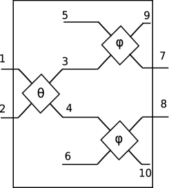
Figure 1: Polarization mixing and losses are modeled by three beam splitters characterized by real random variables $\theta$ and $\phi$ which have the probability distribution $P(\theta,\phi)$. Input states enter the channel in modes $1$ and $2$ and the output is read in modes $7$ and $8$.

Let us consider a laser pulse which first passes through a polarization beam splitter to separate two polarizations, e.g. horizontal and vertical, and then is sent through a fiber. Due to imperfections on the fiber, the two polarizations do not necessarily remain distinct, but they tend to become mixed. At the same time along the travel on the fiber the pulse tends to be attenuated. This attenuation effect can be related to the polarization mixing effect. The situation can be modeled by three beam splitters as shown in figure (1).

In general the evolution operator of a beam splitter is given by the unitary transform

$$U(\zeta)=e^{\zeta ab^{{\dagger}}-\zeta^{*}a^{{\dagger}}b},$$ (1)

depending on a complex parameter $\zeta$. Here $a$ ($a^{{\dagger}}$) and $b$ ($b^{{\dagger}}$) are annihilation (creation) operators for the two input radiation modes. It is easy to show that the Heisenberg evolution of the creation operators of the two modes of the input state is given by

$$U(\zeta)\left(\begin{array}[]{c}a^{{\dagger}}\cr b^{{\dagger}}\cr\end{array}\right)U^{{\dagger}}(\zeta)=\left(\begin{array}[]{cc}\cos|\zeta|&e^{i\arg\zeta}\sin|\zeta|\cr-e^{-i\arg\zeta}\sin|\zeta|&\cos|\zeta|\end{array}\right)\left(\begin{array}[]{c}a^{{\dagger}}\cr b^{{\dagger}}\cr\end{array}\right).$$ (2)

All the beam splitters in the channel are characterized by real parameters $\theta$ and $\phi$. Labeling the creation operators of the input modes by $a_{1}^{{\dagger}}$ and $a_{2}^{{\dagger}}$ and using equation (2), the creation operators of modes 3 and 4 in figure are given by

$$a_{3}^{{\dagger}} = \cos\theta a_{1}^{{\dagger}}+\sin\theta a_{2}^{{\dagger}}$$ (3)

$$a_{4}^{{\dagger}} = -\sin\theta a_{1}^{{\dagger}}+\cos\theta a_{2}^{{\dagger}},$$ (4)

which shows that they are a mixture of modes 1 and 2, hence the polarization mixing effect. For example, if the mode 1 (2) denotes the horizontal-polarized (vertical-polarized) photons, in mode 3 (4) photons with both horizontal and vertical polarization will appear.

Then, each output of the first beam splitter goes through another beam splitter, characterized by a real parameter $\phi$, and interacts with environment in the vacuum state. This part models the losses in the channel with a loss rate equal to $\sin^{2}\phi$.

The total action of these three beam splitters on the input state $\rho_{1,2}$ is described by the map

$$\Phi_{\theta,\phi}(\rho_{1,2})={\rm Tr}_{env}\left[U_{4,6}(\phi)U_{3,5}(\phi)U_{1,2}(\theta)(\rho_{1,2}\otimes|00\rangle_{3,4}\langle 00|)U^{{\dagger}}_{1,2}(\theta)U^{{\dagger}}_{3,5}(\phi)U^{{\dagger}}_{4,6}(\phi)\right],$$ (5)

where the environment modes are labeled by indices $5$ and $6$. To complete the definition of the channel we introduce correlation between polarization mixing (characterized by $\theta$) and losses (characterized by $\phi$). This can be done by means of a joint probability distribution $P(\theta,\phi)$ for the values that $\theta$ and $\phi$ can take. Thus, the output of the channel results

$$\Phi(\rho)=\int d\theta d\phi P(\theta,\phi)\Phi_{\theta,\phi}(\rho).$$ (6)

We assume $P(\theta,\phi$) to be a Gaussian distribution of the following form:

$$P(\theta,\phi)=\frac{1}{2\pi\sigma^{2}\sqrt{|\gamma^{-1}}|}e^{-\frac{1}{2\sigma^{2}}r^{t}\gamma r},$$ (7)

where $r=(\theta-\theta^{*},\phi-\phi^{*})^{t}$ and $\gamma$ is the correlation matrix:

$$\gamma=\left(\begin{array}[]{cc}1&-x\cr-x&1\end{array}\right).$$ (8)

The parameter $x\in[0,1]$ accounts for the degree of correlation between the two effects (polarization mixing and loss). For $x=0$ we have

$$P(\theta,\phi)=p(\theta)p(\phi)$$ (9)

where $p(\theta)$ and $p(\phi)$ are independent and identical probability distributions

$$p(\theta)=\frac{1}{\sqrt{2\pi\sigma^{2}}}e^{-\frac{(\theta-\theta^{*})^{2}}{2\sigma^{2}}},\hskip 28.45274ptp(\phi)=\frac{1}{\sqrt{2\pi\sigma^{2}}}e^{-\frac{(\phi-\phi^{*})^{2}}{2\sigma^{2}}}.$$ (10)

They are characterized by mean values $\theta^{*}$ and $\phi^{*}$ and variance $\sigma^{2}$. By increasing $x$, the distance between the probability distributions $P(\theta,\phi)$ and $p(\theta)p(\phi)$ increases,

$$\left|P(\theta,\phi)-p(\theta)p(\phi)\right|=p(\theta)p(\phi)\left|1-e^{-\frac{1}{2\sigma^{2}}(\theta-\theta^{*})(\phi-\phi^{*})x}\right|.$$ (11)

This can be interpreted as increasing the correlation KMM . Since at $x=1$ the maximum of the joint probability distribution is at $\theta-\theta^{*}=\phi-\phi^{*}$ we consider it as the most correlated case.

The last remark which is necessary on the probability distribution (7) is that it is not a periodic function of $\theta$ and $\phi$, while the beam splitter operators are periodic in $\theta\in[-\pi,\pi]$ and $\phi\in[-\pi,\pi]$. Hereafter we assume the variance $\sigma$ of the probability distribution to be sufficiently small ($\ll 2\pi$), so that boundary effects due to the periodicity become negligible.

Our aim is to study the one-shot classical capacity for the channel (6) and analyse how it behaves with respect to the correlation parameter $x$. By definition, it is given by HSW :

$$C=\sup_{\{p_{i},\rho_{i}\}}\chi(\Phi(\rho_{i},p_{i})),$$ (12)

where the supremum is taken over all possible ensemble of input states, namely$\{p_{i},\rho_{i}\}$ and $\chi$ is the Holevo information

$$\chi(\rho)=S\left(\Phi\left(\sum_{i}p_{i}\rho_{i}\right)\right)-\sum_{i}p_{i}S\left(\Phi\left(\rho_{i}\right)\right),$$ (13)

with $S$ the von-Neumann entropy.

In the following we are going to consider classical information over a continuous alphabet encoded in weak coherent states as well as classical information over a discrete alphabet encoded into qubit states.

III Weak coherent input

Since coherent states turns out to be optimal for achieving the capacity in lossy bosonic channels GioPRL92 , we consider them as input to the channel (6). A coherent state of complex amplitude $\alpha$ is expressed in the Fock basis by

$$|\alpha\rangle=e^{-\frac{|\alpha|^{2}}{2}}\sum_{n=0}^{\infty}\frac{\alpha^{n}}{\sqrt{n!}}|n\rangle.$$ (14)

We are here interested on weak (attenuated) coherent states which likely contain no photon or one photon, i.e. they are characterized by an amplitude $|\alpha|\ll 1$. To provide the two input modes of the channel in figure (1), we consider horizontal and vertical-polarized photons so that the state of modes $1$ and $2$ in figure 1 can be written as

$$|\alpha\rangle\approx N(|00\rangle_{1,2}+\alpha(|01_{{}_{V}}\rangle_{1,2}+|1_{{}_{H}}0\rangle_{1,2}))$$ (15)

where $N=\frac{1}{\sqrt{1+2|\alpha|^{2}}}$ represents the normalization factor.

It is straightforward to show that the state (15) will be transformed to the following state after the action of the first beam splitter:

$$N[|00\rangle+\alpha\cos\theta(|01_{{}_{V}}\rangle+|1_{{}_{H}}0\rangle)-\alpha\sin\theta(|01_{{}_{H}}\rangle-|1_{{}_{V}}0\rangle)]_{3,4}$$ (16)

(17)

$$\quad=\cos\theta|\alpha\rangle_{3,4}-N[\cos\theta|00\rangle+\alpha\sin\theta(|01_{{}_{H}}\rangle-|1_{{}_{V}}0\rangle)]_{3,4}.$$ (18)

In the second step, the above state (18) interacts with modes $5$ and $6$ which are initially in the vacuum. Hence, we have

$$N[|0000\rangle + \alpha\cos\theta\cos\phi(|01_{{}_{V}}00\rangle+|1_{{}_{H}}000\rangle)$$ (19)

$$- \alpha\cos\theta\sin\phi(|0001_{{}_{V}}\rangle+|001_{{}_{H}}0\rangle)$$ (20)

$$- \alpha\sin\theta\cos\phi(|01_{{}_{H}}00\rangle-|1_{{}_{V}}000\rangle)$$ (21)

$$+ \alpha\sin\theta\sin\phi(|0001_{{}_{H}}\rangle-|001_{{}_{V}}0\rangle)]_{7,8,9,10}.$$ (22)

By introducing

$$|f(\alpha)\rangle := |00\rangle+\alpha|01_{{}_{H}}\rangle-\alpha|1_{{}_{V}}0\rangle,$$ (23)

$$g(\theta,\phi) := 1-(\cos\theta-\sin\theta)(\cos\phi-\sin\phi),$$ (24)

we can rewrite the state (22) in the following form:

$$|\Psi\rangle=N [ g(\theta,\phi)|0000\rangle_{7,8,9,10}+\cos\theta\cos\phi|\alpha\rangle_{7,8}|00\rangle_{9,10}-\cos\theta\sin\phi|00\rangle_{7,8}|\alpha\rangle_{9,10}$$ (25)

$$- \sin\theta\cos\phi|f(\alpha)\rangle_{7,8}|00\rangle_{9,10}+\sin\theta\sin\phi|00\rangle_{7,8}|f(\alpha)\rangle_{9,10}],$$ (27)

which shows that with some probability the input state $|\alpha\rangle$ emerges at the output modes $7$ and $8$. However, there is a chance of loosing all the photons to the environment, and a chance that, though the photons do not go to the environment, the output state $|f(\alpha)\rangle$ is different from the input one.

To find the final state which represents the channel output we trace $|\Psi\rangle\langle\Psi|$ over modes $9$ and $10$ and then integrate over $\theta$ and $\phi$ as in (6), thus obtaining

$$\Phi\left(|\alpha\rangle\langle\alpha|\right)=N^{2}\left(\begin{array}[]{ccccc}1+2|\alpha|^{2}(1-\mathcal{A}-\mathcal{B})&\bar{\alpha}\mathcal{D}&\bar{\alpha}\mathcal{D}&-\bar{\alpha}\mathcal{E}&-\bar{\alpha}\mathcal{E}\cr\alpha\mathcal{D}&|\alpha|^{2}\mathcal{A}&|\alpha|^{2}\mathcal{A}&-\frac{1}{2}|\alpha|^{2}\mathcal{C}&-\frac{1}{2}|\alpha|^{2}\mathcal{C}\cr\alpha\mathcal{D}&|\alpha|^{2}\mathcal{A}&|\alpha|^{2}\mathcal{A}&-\frac{1}{2}|\alpha|^{2}\mathcal{C}&-\frac{1}{2}|\alpha|^{2}\mathcal{C}\cr-\alpha\mathcal{E}&-\frac{1}{2}|\alpha|^{2}\mathcal{C}&-\frac{1}{2}|\alpha|^{2}\mathcal{C}&|\alpha|^{2}\mathcal{B}&|\alpha|^{2}\mathcal{B}\cr-\alpha\mathcal{E}&-\frac{1}{2}|\alpha|^{2}\mathcal{C}&-\frac{1}{2}|\alpha|^{2}\mathcal{C}&|\alpha|^{2}\mathcal{B}&|\alpha|^{2}\mathcal{B}\cr\end{array}\right),$$ (28)

where $\mathcal{A},\mathcal{B},\mathcal{C},\mathcal{D}$ and $\mathcal{E}$ are real functions of $\theta^{*},\phi^{*},\sigma$ and $x$ whose explicit form is given in Appendix. It is important to note that the order of $|\alpha|$ is the same in the output state and the input state $|\alpha\rangle\langle\alpha|$.

Once we have the output state of the channel we can then evaluate the Holevo information. We recall that the Holevo information for an ensemble $\mathfrak{S}=\{|\alpha\rangle;\;\wp(\alpha)\}$ of input states corresponding to a continuous alphabet is given by:

$$\chi(\mathfrak{S})=S(\tilde{\rho})-\int d^{2}\alpha\wp(\alpha)S\left(\Phi(|\alpha\rangle\langle\alpha|)\right),$$ (29)

in which $\wp$ is a probability distribution and $\tilde{\rho}$ is the average output state

$$\tilde{\rho}=\Phi\left(\int d^{2}\alpha\wp(\alpha)|\alpha\rangle\langle\alpha|\right)=\int d^{2}\alpha\wp(\alpha)\Phi\left(|\alpha\rangle\langle\alpha|\right).$$ (30)

We restrict the ensemble of input states to that of weak coherent states (15) with Gaussian distribution $\wp(\alpha)$:

$$\wp(\alpha)=\frac{1}{2\pi\Delta^{2}}e^{-\frac{|\alpha|^{2}}{2\Delta^{2}}}.$$ (31)

The variance $\Delta^{2}$ should be chosen in a way that the ensemble of input states only includes weak coherent states, i.e. $\Delta\ll 1$. We also know that $\theta$ and $\phi$ are random variables with Gaussian probability distribution centered around $\theta^{*}$ and $\phi^{*}$ with variance $\sigma$. Therefore to have the channel close to an ideal transmitter, we assume narrow probability distributions (small $\sigma$) centered around $\theta^{*}=\phi^{*}=0$. Under these assumptions $\mathcal{C}=\mathcal{E}\approx 0$, therefore the output of the channel (28) is block diagonal with the following eigenvalues:

$$\lambda_{1,2} = \frac{N^{2}}{2}(1+2|\alpha|^{2}-2|\alpha|^{2}\mathcal{B}\pm\sqrt{(1-2|\alpha|^{2}\mathcal{A})^{2}+8|\alpha|^{2}\mathcal{D}},$$ (32)

$$\lambda_{3} = 2N^{2}|\alpha|^{2}\mathcal{B},$$ (33)

$$\lambda_{4,5} = 0.$$ (34)

Using these eigenvalues the output entropy

$$S\left(\Phi(|\alpha\rangle\langle\alpha|)\right)=-\sum_{i=1}^{5}\lambda_{i}\log\lambda_{i},$$ (35)

can be easily expressed analytically. Nevertheless, the integral in the second term of the Holevo information (29) should be computed numerically.

For finding the first term of Holevo information we note that $\wp(\alpha)$ is even in $\alpha$, therefore the average output state is block diagonal

$$\tilde{\rho}=\left(\begin{array}[]{ccccc}1-2\mathcal{L}(\mathcal{A}+\mathcal{B})&&&&\cr&\mathcal{A}\mathcal{L}&\mathcal{A}\mathcal{L}&&\cr&\mathcal{A}\mathcal{L}&\mathcal{A}\mathcal{L}&&\cr&&&\mathcal{B}\mathcal{L}&\mathcal{B}\mathcal{L}\cr&&&\mathcal{B}\mathcal{L}&\mathcal{B}\mathcal{L}\end{array}\right),$$ (36)

with the following eigenvalues:

$$\tilde{\lambda}_{1} = 1+2\mathcal{L}(1-\mathcal{A}-\mathcal{B}),$$ (37)

$$\tilde{\lambda}_{2} = 2\mathcal{A}\mathcal{L},$$ (38)

$$\tilde{\lambda}_{3} = 2\mathcal{B}\mathcal{L},$$ (39)

$$\tilde{\lambda}_{4,5} = 0,$$ (40)

and

$$\mathcal{L}=\int d^{2}\alpha\wp(\alpha)\frac{|\alpha|^{2}}{1+2|\alpha|^{2}}.$$ (41)

Evaluating $\mathcal{L}$ numerically the first term of Holevo information in equation (29)

$$S(\tilde{\rho})=-\sum_{i}\tilde{\lambda}_{i}\log\tilde{\lambda}_{i},$$ (42)

can also be found. The final result for Holevo information (29) is plotted in figure (2) versus the correlation parameter $x$, for different values of $\sigma$. It shows that the Holevo information for the ensemble of input states (31) is a decreasing function of correlation parameter $x$. For $x=0$ polarization mixing and loss happen independently, therefore there is the chance that just one of them happens. By increasing the correlation parameter the probability that both errors happen increases and therefore the rate of information transmission decreases. As it is clear from the figure (2), by decreasing $\sigma$ the Holevo quantity increases, this reflects the fact the narrow the probability distribution is, the less is the noise in the channel. As $\sigma$ goes to $0$, $\mathcal{A},\mathcal{D}\rightarrow 1$ and $\mathcal{B}\rightarrow 0$. In this case the output state gets closer to a pure state of the form of input state (15).

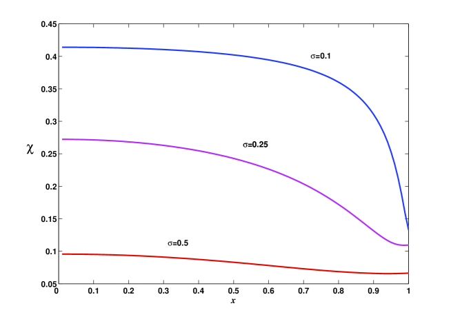
Figure 2: Holevo information versus correlation parameter $x$ when information is encoded in weak coherent states. Different lines are for different values of $\sigma$.

IV Qubit inputs

In this section we use qubit encoding in single photons. To this end we consider the two input modes 1 and 2 to only have one photon in total. Therefore the photon is either in mode 1 or in mode 2 and a general input pure state is given by:

$$|\psi\rangle=c_{0}|01\rangle+c_{1}|10\rangle,$$ (43)

with $c_{0},c_{1}$ are complex coefficient such that $|c_{0}|^{2}+|c_{1}|^{2}=1$. By referring to the dual-rail coding

$$|0\rangle_{L}\leftrightarrow|01\rangle_{1,2}\hskip 28.45274pt|1\rangle_{L}\leftrightarrow|10\rangle_{1,2}.$$ (44)

it is clear that the state in (43) represent a general pure state for a single logical qubit.

Our aim is to find the capacity of channel (6) when we encode information in qubits. The upper bound of Holevo information (13) is given by

$$\chi\leq 1-S(\Phi(\rho^{*})),$$ (45)

in which $\rho^{*}$ is an input state with minimum output entropy M3 . Using the concavity property of entropy, it has been shown that for finding the input state with minimum output entropy it is enough to search among the pure states M3 . Therefore we consider the input ensemble that includes pure states of form (43). Using equation (2) it is easy to show that

$$U(\theta)|01\rangle = \cos\theta|01\rangle-\sin\theta|10\rangle,$$ (46)

$$U(\theta)|10\rangle = \sin\theta|01\rangle+\cos\theta|10\rangle,$$ (47)

therefore the action of the first beam splitter is a rotation by angle $\theta$ in the $|0\rangle_{L}$ and $|1\rangle_{L}$ plain, and the input state

$$|\psi\rangle_{L}=c_{0}|0\rangle_{L}+c_{1}|1\rangle_{L},$$ (48)

will be transformed to

$$|\psi(\theta)\rangle_{L}=e^{-i\theta\sigma_{y}}|\psi\rangle_{L},$$ (49)

in which $\sigma_{y}$ is the $y$ Pauli operator. The dual-rail state at the output modes of the first beam splitter is then given by

$$(c_{0}\cos\theta+c_{1}\sin\theta)|01\rangle_{3,4}-(c_{0}\sin\theta-c_{1}\cos\theta)|10\rangle_{3,4}.$$ (50)

This state interacts with modes $5$ and $6$ which are in the vacuum and will be transformed into

$$(c_{0}\cos\theta+c_{1}\sin\theta)[\sin\phi|0001\rangle+\cos\phi|0100\rangle]_{7,8,9,10}$$ (51)

$$- (c_{0}\sin\theta-c_{1}\cos\theta)[\sin\phi|0010\rangle+\cos\phi|1000\rangle]_{7,8,9,10}.$$ (52)

If we take $|2\rangle_{L}\leftrightarrow|00\rangle$, then the output state of system and environment can be summarized as follows:

$$\sin\phi|2_{s}\rangle_{L}|\psi(\theta)_{e}\rangle_{L}+\cos\phi|\psi(\theta)_{s}\rangle_{L}|2_{e}\rangle_{L},$$ (53)

where $s$ and $e$ are labels for system and environment respectively. Tracing over the environment and taking into account the correlation between the parameters of the beam splitters the final output state of the channel is:

$$\Phi(|\psi\rangle_{L}\langle\psi|)=\epsilon|2\rangle_{L}\langle 2|+(1-\epsilon)e^{-i\theta^{*}\sigma_{y}}|\psi\rangle_{L}\langle\psi|e^{i\theta^{*}\sigma_{y}},$$ (54)

where

$$\epsilon=\int\sin^{2}\phi P(\theta,\phi)d\theta d\phi=\frac{1}{2}\left(1-\cos 2\phi^{*}e^{-\frac{2\sigma^{2}}{1-x^{2}}}\right).$$ (55)

Since $|2\rangle_{L}$ is orthogonal to the manifold of the input states, equation (54) shows that the information is lost with probability $\epsilon$ and the state is rotated by average angle $\theta^{*}$ with probability $(1-\epsilon)$. Therefore the total map is a kind of a quantum erasure channel erasure and its capacity is given by

$$C=(1-\epsilon)C_{\Omega},$$ (56)

where $C_{\Omega}$ is the capacity of the the channel $\Omega$

$$\Omega(\rho)=e^{-i\theta^{*}\sigma_{y}}\rho e^{i\theta^{*}\sigma_{y}}.$$ (57)

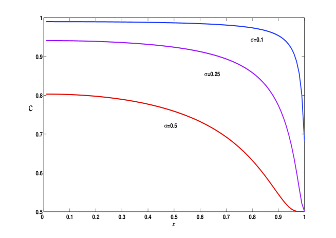
Figure 3: Classical capacity of the channel versus correlation parameter $x$ when information is encoded into qubits. Different lines are for different values of $\sigma$.

Since $\Omega$ is a rotation about $y$ axis it is obvious that the following states remain invariant under its action:

$$|\psi_{1,2}\rangle_{L}=\frac{1}{\sqrt{2}}(|0\rangle_{L}\pm i|1\rangle_{L}),$$ (58)

thus giving zero output entropy and minimizing the second term of Holevo information.

It is easy to show that if these states are used with equal probability in the ensemble of input state then

$$\frac{1}{2}\Omega(|\psi_{1}\rangle_{L}\langle\psi_{1}|)+\frac{1}{2}\Omega(|\psi_{2}\rangle_{L}\langle\psi_{2}|)=\frac{1}{2}I.$$ (59)

Therefore this ensemble also maximizes the first term in Holevo information and $C_{\Omega}=1$ can be achieved by using the above states to encode information. As a consequence the capacity of the channel $\Phi$ results $C=(1-\epsilon)$.

Figure (3) shows this capacity versus the correlation parameter $x$ for different values of $\sigma$ when $\theta^{*}=\phi^{*}=0$. At $x=0$ the values of $\phi$ which are close to $0$ are the most probable values, however by increasing $x$ the higher values of $\phi$ also have chance to happen. Therefore the probability of loosing information increases and as it is seen in figure (3) the capacity of the channel decreases. By decreasing $\sigma$ the probability distribution becomes more and more narrow and the chance for having values of $\phi$ far from $\phi^{*}=0$ become less. Therefore the channel capacity increases by decreasing the variance of probability distribution which can be seen in figure (3).

V conclusion

We have provided a model of quantum channel with correlated errors of different kinds. While correlation in errors between different uses of channels have been studied before, in our model different types of correlated errors happen in each use of the channels on different degrees of freedom. This assumption can be justified by considering practical situations i. e. optical fibers where photon loss and polarization errors may be correlated. Actually our model describes photon losses depending on the degree of polarization mixedness.

On the one hand, for classical information over a continuous alphabet we have considered weak coherent states and we have shown that the Holevo information decreases by increasing the correlation between polarization mixdness and losses. On the other hand, for classical information over a discrete alphabet we have considered single photons using dual rail representation. In this case we have shown that the channel is kind of quantum erasure channel where the probability of erasing information increases with the polarization mixdness. It is worth remarking that while often memory effects lead to an enhancement of the channel capacity, in the present model exactly the opposite happens. This is mainly due to the fact that the polarization mixing alone cannot be considered as a “true” error, i.e. it is not due to the action of an environment.

In conclusion, we are confident that this work may pave the way for characterizing realistic quantum channels where different degrees of freedom and different effect are involved.

Appendix

To evaluate the quantities $\mathcal{A}$, $\mathcal{B}$, $\mathcal{C}$, $\mathcal{D}$ and $\mathcal{E}$ in (28) we use the fact that the variance of the probability distribution $P(\theta,\phi)$ is sufficiently smaller than $2\pi$, hence we can extend the limits of the integrals to $(-\infty,\infty)$ treating them like standard Gaussian integrals, thus obtaining:

$$\mathcal{A} = \int\cos^{2}\theta\cos^{2}\phi P(\theta,\phi)d\theta d\phi$$ (60)

$$= \frac{1}{4}\left(1+e^{-\frac{2\sigma^{2}}{1-x^{2}}}(\cos 2\theta^{*}+\cos 2\phi^{*})+\frac{1}{2}(e^{-\frac{4\sigma^{2}}{1-x}}+e^{-\frac{4\sigma^{2}}{1+x}})\cos 2\theta^{*}\cos 2\phi^{*}\right),$$ (61)

$$\mathcal{B} = \int\sin^{2}\theta\cos^{2}\phi P(\theta,\phi)d\theta d\phi$$ (63)

$$= \frac{1}{4}\left(1-e^{-\frac{2\sigma^{2}}{1-x^{2}}}(\cos 2\theta^{*}-\cos 2\phi^{*})-\frac{1}{2}(e^{-\frac{4\sigma^{2}}{1-x}}+e^{-\frac{4\sigma^{2}}{1+x}})\cos 2\theta^{*}\cos 2\phi^{*}\right),$$ (64)

$$\mathcal{C} = \int\sin 2\theta\cos^{2}\phi P(\theta,\phi)d\theta d\phi=\frac{1}{4}\left(2e^{-\frac{2\sigma^{2}}{1-x^{2}}}-(e^{-\frac{4\sigma^{2}}{1-x}}+e^{-\frac{4\sigma^{2}}{1+x}})\cos\phi^{*}\right)\sin 2\theta^{*},$$ (66)

$$\mathcal{D} = \int\cos\theta\cos\phi P(\theta,\phi)d\theta d\phi=\frac{1}{2}\left(e^{-\frac{\sigma^{2}}{1-x}}+e^{-\frac{\sigma^{2}}{1+x}}\right)\cos\theta^{*}\cos\phi^{*},$$ (68)

$$\mathcal{E} = \int\sin\theta\cos\phi P(\theta,\phi)d\theta d\phi=\frac{1}{2}\left(e^{-\frac{\sigma^{2}}{1-x}}+e^{-\frac{\sigma^{2}}{1+x}}\right)\sin\theta^{*}\cos\phi^{*}.$$ (70)

References

- (1) C. King, quant-ph/0103156; M. B. Hastings, Nat. Phys. 5, 255 (2009); T. Cubitt, A. W. Harrow, D. Leung, A. Montanaro and A. Winter, Comm. Math. Phys. 284, 281 (2008); G. G. Amosov and S. Mancini, Quant. Inf. & Comp. 9, 594 (2009).
- (2) D. Kretschmann and R. F. Werner, Phys. Rev. A 72, 062323 (2005).
- (3) C. Macchiavello, and G.M. Palma, Phys. Rev. A 65, 050301(R) (2002).
- (4) C. Macchiavello, G. M. Palma, and S. Virmani, Phys. Rev. A 69, 010303 (2004).
- (5) E. Karpov, D. Daems, N. J. Cerf, Phys. Rev. A 74, 032320 (2006); V. Karimipour and L. Memarzadeh, Phys. Rev. A 74, 032332 (2006).
- (6) K. Banaszek, A. Dragan, W. Wasilewski, and C. Radzewicz, Phys. Rev. Lett. 92, 257901 (2004).
- (7) V. Giovannetti, S. Mancini, Phys. Rev. A 71, 062304 (2005); G. Ruggeri, G. Soliani, V. Giovannetti, S. Mancini, Europhys. Lett. 70, 719 (2005); O. V. Pilyavets, V. G. Zborovskii and Stefano Mancini, Phys. Rev. 77, 052324 (2008); C. Lupo, O. Pilyavets and S. Mancini, New J. Phys. 11, 063023 (2009).
- (8) N. J. Cerf, J. Clavareau, Ch. Macchiavello, J. Roland, Phys. Rev. A 72, 042330 (2005); G. Ruggeri and S. Mancini, Quant. Inf. & Comp. 7, 265 (2007).
- (9) V. Giovannetti, S. Guha, S. Lloyd, L. Maccone, J. H. Shapiro, and H. P. Yuen, Phys. Rev. Lett. 92, 027902 (2004).
- (10) N. Gisin, R. Passy, P. Blasco, M. O. Van Deventer, R. Distl, H. Gilgen, B. Perny, R. Keys, E. Krause, C. C. Larsen, K. Mori, J. Pelayo and J. Vobian, Pure Appl. Opt. 4, 511 (1995)
- (11) Ch. H. Bennett, D. P. DiVincenzo and J. A. Smolin, Phys. Rev. Lett. 78, 3217 (1997).
- (12) V. Karimipour, Z. Meghdadi, and L. Memarzadeh, Phys. Rev. A 79, 032321 (2009);
- (13) A. S. Holevo, IEEE Trans. Inf. Th. 44, 269 (1998); B. Schumacher and M. D. Westmoreland, Phys.Rev. A 56, 131 (1997).