Adiabatic Charge Pumping through Quantum Dots in the Coulomb Blockade Regime

Abstract

We investigate the influence of the Coulomb interaction on the adiabatic pumping current through a quantum dot. Using nonequilibrium Green’s functions techniques, we derive a general expression for the current based on the instantaneous Green’s function of the dot. We apply this formula to study the dependence of the charge pumped per cycle on the time-dependent pumping potentials. Motivated by recent experiments, the possibility of charge quantization in the presence of a finite Coulomb repulsion energy is investigated.

I Introduction

The basic idea of electron pumping, put forward in the pioneer work of Thouless, thouless is to generate a DC current through a conductor in the absence of an applied bias voltage. This may be accomplished by applying time-dependent perturbations to the conductor. In electronic transport through mesoscopic conductors, the typical experimental time scale over which these external perturbations vary is large compared to the lifetime of the electron inside the conductor (dwell time). In that case, the pumping mechanism is called adiabatic.

Adiabatic quantum pumping in mesoscopic noninteracting open quantum dots was investigated theoretically by Brouwer brouwer98 by means of a scattering approach. Applying the emissivity theory introduced by Büttiker and co-workers,buttiker94 he demonstrated that the pumping current is proportional to the driving frequency and shows large mesoscopic fluctuations accounted by Random Matrix Theory. This scattering approach has been employed to investigate several aspects of adiabatic quantum pumping in noninteracting systems, such as the role of discrete symmetries on the pumped charge,aleiner00 the effects of inelastic scattering and decoherence,MoskButt01 ; cremers02 the role of noise and dissipation,MoskButt02 Andreev interference effects in the presence of superconducting leads,tadei04 ; blaauboer02 as well as spin pumping.mucciolo02 ; governale03 ; moises04 ; Mucciolo07 Pumping phenomena in noninteracting systems have also been investigated using alternative theoretical approaches, such as the formalism based on iterative solutions of time-dependent statesentin02 and the Keldysh formulation.vavilov01 Both approaches can be used beyond the adiabatic approximation.

Experimentally, the first implementation of an electron pump was due to Pothier et al. when charge was quantized due to Coulomb blockade (CB) effects.pothier92 Adiabatic phase-coherent charge pumping, though not quantized, was observed in open semiconductor quantum dots switkes99 and in carbon nanotube quantum dots.Leek05 ; Buitelaar08 Quantized charge pumping was recently observed in AlGaAs/GaAs nanowires using a single-parameter modulation,kaestner08 a result with potential applications to metrology. An experimental realization of a quantum spin pump has also been implemented.watson03

Pumping through interacting systems, where the scattering approach does not apply, has been much less studied so far. Using the slave-boson mean-field approximation, Aono investigated the spin-charge separation of adiabatic currents in the Kondo regime.aono04 The behavior of the pumping current through a quantum dot in the Kondo regime was studied both for adiabaticSchiller08 and nonadiabatic systemsArrachea08 using the Keldysh formalism. Quantum pumping was investigated both in the CB regime brouwer05 ; cota05 as well as for almost open quantum dots. aleiner98 The nonequilibrium Green’s functions technique has been employed to investigate adiabatic pumping through interacting quantum dots in infinite $U$ systems.Splettstoesser05 ; sela06 The role of the Coulomb interaction in the adiabatic pumping current has also been investigated in the limit of weak tunneling and infinite-$U$ using diagrammatic techniques.Splettstoesser06 The presence of electron-electron interactions was shown to improve charge quantization in one-dimensional disordered wires under certain circumstances.Devillard08 The effects of the coupling of the quantum dot to bosonic environments and its implications to charge quantization were analyzed in Ref. Fioretto08, . The interplay of nonadiabacity and interaction effects on the pumping current were also recently reported.Braun08 ; Cavalieri09

In the present paper we investigate adiabatic charge pumping through interacting quantum dots in the CB regime for temperatures much higher than the Kondo temperature. We consider quantum dots with a single level subjected to a finite Coulomb repulsion $U$ in the case of double occupancy. We investigate the time dependence of the pumping current by keeping $U$ finite, a scenario out of the domain of validity of the theory developed in Refs. Splettstoesser05, and sela06, . This allows us to identify the relevant time scales controlling the current amplitude in realistic situations. We develop a general formalism, based on non-equilibrium Green’s functions, to investigate the influence of the Coulomb interaction on the adiabatic pumping current. We discuss some applications and consequences of this formulation and evaluate several quantities of interest numerically for a range of parameters. Finally, the possibility of charge quantization in the presence of a finite Coulomb repulsion is investigated. The study of charge quantization in the adiabatic regime is interesting by its own, and is also a necessary step towards the understanding of recent experimentskaestner08 dealing with non-adiabatic pumping.

This paper is organized as follows. In Section II we present the model used to calculate the time-dependent current flowing through the quantum dot. Section III is devoted to the explicit calculation of the relevant Green’s functions. In Section IV, we apply this calculation to derive an expression for the pumping current in the adiabatic approximation for systems with finite $U$. The numerical evaluation of the current as well as a discussion of its consequences and implications is presented in Section V. Finally, Section VI is devoted to a brief summary of our findings and concluding remarks.

II Model for transport in quantum dots

We consider a quantum dot (QD) with a single, isolated resonance in the Coulomb blockade regime, as schematically depicted in Fig. 1. The potential in the dot is controlled by a time-dependent gate voltage $V_{g}(t)$ such that the QD Hamiltonian reads

$$H_{\rm dot}=\sum_{s=\uparrow,\downarrow}\varepsilon_{s}(t)\,d^{\dagger}_{s}d_{s}+U\,n_{\uparrow}n_{\downarrow},$$ (1)

where $n_{s}=d^{\dagger}_{s}d_{s}$ is the number operator and $d^{\dagger}_{s}$ ($d_{s}$) is the creation (annihilation) operator for an electron with energy $\varepsilon_{s}(t)=\varepsilon_{0s}-\eta\,eV_{g}(t)$ and spin $s$ in the QD. Here, $e$ denotes the electron charge and $\eta$ is a lever arm factor for the gate voltage. Two single-channel leads are attached to the QD. It is assumed that electrons in the leads are noninteracting and obey the Hamiltonian

$$H_{\rm lead}=\sum_{k}\sum_{\alpha={\rm L,R}}\sum_{s=\uparrow,\downarrow}\varepsilon_{k\alpha s}\,c^{\dagger}_{k\alpha s}c_{k\alpha s}\,,$$ (2)

where $c^{\dagger}_{k\alpha s}$ and $c_{k\alpha s}$ are, respectively the creation and annihilation operators for electrons with momentum $k$ and spin $s$ in the lead $\alpha$. The QD is separated from the leads by tunneling barriers controlled by the lateral gates $V_{1}$ and $V_{2}$ (see Fig. 1). The coupling Hamiltonian reads

$$H_{\rm lead-dot}=\sum_{k,\alpha,s}\left[V_{k\alpha}(t)\,c_{k\alpha s}^{\dagger}d_{s}+\rm{H.c.}\right].$$ (3)

The tunneling matrix elements $V_{k\alpha}$ connect states in the leads to the resonant state in the dot and are assumed to be spin independent. The total Hamiltonian of our model is the sum of these three contributions,

$${\cal H}=H_{\rm lead}+H_{\rm dot}+H_{\rm lead-dot}.$$ (4)

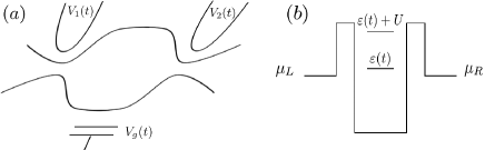
Figure 1: (a) Schematic view of a two-contact quantum dot coupled to a time-dependent gate. (b) Sketch of the energy levels of the model described in the text.

The coupling between the states in the leads and those in the dot, combined with the dot charging energy, turns the time evolution of the system into a nontrivial many-body problem. As a result, we cannot apply a single-particle formalism to describe the transport through the system and the usual scattering-matrix formulation for pumping currents brouwer98 is inappropriate. To circumvent these difficulties, we employ the Schwinger-Keldysh formalism and the equation-of-motion method ramm to calculate the current through an interacting quantum dot in the CB regime.

Our starting point is the general expression for the time-dependent current in terms of the quantum dot Green’s function $G_{s,s}(t,t^{\prime})$:HaugJauho96 ; Jauho94

$$J_{\alpha}(t) \!\!= \!\!-\frac{2e}{\hbar}\ {\rm Im}\Big{\{}\ \sum_{k,s}\int_{-\infty}^{t}dt^{\prime}\,V^{\ast}_{k\alpha}(t^{\prime})e^{i\varepsilon_{k\alpha s}(t-t^{\prime})/\hbar}V_{k\alpha}(t)$$ (5)

$$\times\left[f_{\alpha}(\varepsilon_{k\alpha s})\,G^{r}_{s,s}(t,t^{\prime})+G^{<}_{s,s}(t,t^{\prime})\right]\Big{\}},$$

where $f_{\alpha}(E)=[e^{(E-\mu_{\alpha})/k_{B}T}+1]^{-1}$ is the Fermi function for the lead $\alpha$ maintained at a chemical potential $\mu_{\alpha}$ and temperature $T$ and $k_{B}$ is the Boltzmann constant. Throughout the text we consider pumping in the absence of an external bias, that is, $\mu_{R}=\mu_{L}=\varepsilon_{F}$. For convenience, we set $\varepsilon_{F}=0$. The lesser, retarded, and advanced dot Green’s functions are defined as ramm

$$G^{<}_{s,s}(t,t^{\prime}) \equiv \frac{i}{\hbar}\left\langle d^{\dagger}_{s}(t^{\prime})\,d_{s}(t)\right\rangle,$$

$$G^{r}_{s,s}(t,t^{\prime}) \equiv -\frac{i}{\hbar}\theta(t-t^{\prime})\left\langle\{d_{s}(t),d^{\dagger}_{s}(t^{\prime})\}\right\rangle,$$

$$G^{a}_{s,s}(t,t^{\prime}) \equiv \frac{i}{\hbar}\theta(t^{\prime}-t)\left\langle\{d_{s}(t),d^{\dagger}_{s}(t^{\prime})\}\right\rangle.$$ (6)

Now it remains to compute the Green’s function $G_{s,s}(t,t^{\prime})$ which involves the quantum dot states. This is where the many-body aspects of the problem make their way into the pumping current. Section III is devoted to this issue.

III Calculation of $G_{s,s}$

The current in Eq. (5) is given in terms of the quantum dot Green’s functions $G^{r}_{s,s}(t,t^{\prime})$ and $G^{<}_{s,s}(t,t^{\prime})$. To write expressions for them, we start by calculating the time-ordered Green’s function $G_{s,s}(t,t^{\prime})$, defined as ramm

$$G_{s,s}(t,t^{\prime})\equiv-\frac{i}{\hbar}\left\langle{\cal T}\!\left[d_{s}(t)\,d^{\dagger}_{s}(t^{\prime})\right]\right\rangle,$$ (7)

where ${\cal T}$ is the time-ordering operator. The equation-of-motion for $G_{s,s}$ is

$$\!\!\!\left[i\hbar\frac{\partial}{\partial t}-\varepsilon_{s}(t)\right]G_{s,s}(t,t^{\prime}) = \delta(t-t^{\prime})+U\,G^{(2)}_{s\bar{s},s}(t,t^{\prime})$$ (8)

$$+ \sum_{k,\alpha}V_{k\alpha}^{\ast}(t)\,G_{k\alpha s,s}(t,t^{\prime}).$$

In Eq. (8) we have introduced the “contact” time-ordered Green’s function

$$G_{s,k\alpha s}(t,t^{\prime})\equiv-\frac{i}{\hbar}\left\langle{\cal T}\left[d_{s}(t)\,c^{\dagger}_{k\alpha s}(t^{\prime})\right]\right\rangle,$$ (9)

which obeys the equation-of-motion

$$\left(-i\hbar\frac{\partial}{\partial t^{\prime}}-\varepsilon_{k\alpha s}\right)G_{s,k\alpha s}(t,t^{\prime})=V_{k\alpha}^{\ast}(t^{\prime})\,G_{s,s}(t,t^{\prime}),$$ (10)

as well as the second-order correlation function

$$G^{(2)}_{s\bar{s},s}(t,t^{\prime})\equiv-\frac{i}{\hbar}\left\langle{\cal T}\!\left[d_{s}(t)\,n_{\bar{s}}(t)\,d^{\dagger}_{s}(t^{\prime})\right]\right\rangle,$$ (11)

that involves four fermionic operators and is generated by the interaction term $Un_{\downarrow}n_{\uparrow}$. The same interaction term leads to the appearance of even higher order correlation functions in the equation-of-motion for $G^{(2)}$, namely,

$$\left[i\hbar\frac{\partial}{\partial t}-\varepsilon_{s}(t)-U\right]G^{(2)}_{s\bar{s},s}(t,t^{\prime})=\delta(t-t^{\prime})\langle n_{\bar{s}}(t)\rangle+\sum_{k\alpha}\left[V_{k\alpha}^{\ast}\Gamma_{1;k\alpha s}^{(2)}(t,t^{\prime})\right]+\sum_{k\alpha}\left[V_{k\alpha}\Gamma_{2;k\alpha s}^{(2)}(t,t^{\prime})-V_{k\alpha}^{\ast}\Gamma_{3;k\alpha s}^{(2)}(t,t^{\prime})\right],$$ (12)

where the occupation number is defined as

$$\langle n_{s}(t)\rangle=\langle d_{s}^{\dagger}(t)d_{s}(t)\rangle\equiv i\hbar\,G_{s,s}^{<}(t,t)$$ (13)

and we have introduced three lead-dot correlation functions,HaugJauho96

$$\Gamma^{(2)}_{1;k\alpha s}(t,t^{\prime})\equiv-\frac{i}{\hbar}\left\langle{\cal T}\!\left[c_{k\alpha s}(t)n_{\bar{s}}(t)d^{\dagger}_{s}(t^{\prime})\right]\right\rangle,$$ (14)

$$\Gamma^{(2)}_{2;k\alpha s}(t,t^{\prime})\equiv-\frac{i}{\hbar}\left\langle{\cal T}\!\left[c^{\dagger}_{k\alpha\bar{s}}(t)d_{s}(t)d_{\bar{s}}(t)d^{\dagger}_{s}(t^{\prime})\right]\right\rangle,$$ (15)

and

$$\Gamma^{(2)}_{3;k\alpha s}(t,t^{\prime})\equiv-\frac{i}{\hbar}\left\langle{\cal T}\!\left[c_{k\alpha\bar{s}}(t)d^{\dagger}_{\bar{s}}(t)d_{s}(t)d^{\dagger}_{s}(t^{\prime})\right]\right\rangle.$$ (16)

At this level, one can verify that the equations-of-motion do not close. Going to the next level, one obtains new (higher order) correlation functions and even more complicated expressions. To solve this problem, we shall recur to an approximate scheme, namely the mean-field approximation.

III.1 Formal solution of the equations-of-motion within the Hartree approximation

We now focus on the Coulomb blockade regime and neglect spin correlations in the leads. That is, we assume that the Kondo temperature,Hewson $T_{K}\sim U\sqrt{\Gamma/2U}\exp\big{(}-\pi|\varepsilon_{s}|(\varepsilon_{s}+U)/2U\Gamma\big{)}$ is very low, $T_{K}\ll T$. As usual, $\Gamma$ stands for the quantum dots resonance linewidth which will be precisely defined in Sec. IV. Hence, with respect to Kondo correlations, we are in the high-temperature regime and the mean-field approximation is expected to be valid. Within this approximation, one can write the $\Gamma^{(2)}$’s as

$$\Gamma^{(2){\rm mf}}_{1;k\alpha s}(t,t^{\prime})=\langle n_{\bar{s}}(t)\rangle\,G_{k\alpha s,s}(t,t^{\prime})$$ (17)

and

$$\Gamma^{(2){\rm mf}}_{2;k\alpha s}(t,t^{\prime})=\Gamma^{(2){\rm mf}}_{3;k\alpha s}(t,t^{\prime})=0.$$ (18)

It has been shown that Kondo correlations are still absent in the next order of the equations-of-motion hierarchical truncation.Meir91 ; HaugJauho96 The latter dresses the Green’s functions self-energies with higher order terms in $V$ that include, for instance, cotunneling processes. As long as $\varepsilon_{s}$ is of the order of $k_{B}T$, we have verified that these contributions give only small corrections to the Hartree mean-field approximation.HaugJauho96 Thus, we write

$$\!\!\!\!\!\!\!\!\!\!\!\!\left[i\hbar\frac{\partial}{\partial t}-\varepsilon_{s}(t)-U\right]G^{(2){\rm mf}}_{s\bar{s},s}(t,t^{\prime})=$$ (19)

$$\langle n_{\bar{s}}(t)\rangle\left[\delta(t-t^{\prime})+\sum_{k\alpha}V_{k\alpha}^{*}(t)\,G_{k\alpha s,s}(t,t^{\prime})\right],$$

where the occupation number $\langle n_{\bar{s}}(t)\rangle$ has to be determined self-consistently for all times. Equations (8), (10), and (19) form a closed set of equations-of-motion that determines the time-ordered Green’s function $G_{s,s}$. Using analytical continuation and the Langreth rules Langreth66 ; HaugJauho96 we can then find the Green’s functions $G^{r}_{s,s}$ and $G^{<}_{s,s}$ that appear in the expressions for the current, Eq. (5). For convenience, let us define two auxiliary time-ordered Green’s functions $g_{s}$ and $g_{s}^{U}$ that obey the equations-of-motions

$$\left[i\hbar\frac{\partial}{\partial t}-\varepsilon_{s}(t)\right]g_{s}(t,t^{\prime})=\delta(t-t^{\prime})$$ (20)

and

$$\left[i\hbar\frac{\partial}{\partial t}-\varepsilon_{s}(t)-U\right]g_{s}^{U}(t,t^{\prime})=\delta(t-t^{\prime}),$$ (21)

respectively. By analytical continuation into the complex plane, we can rewrite Eq. (19) as

$$\!\!\!\!G_{s\bar{s},s}^{(2)\rm{mf}}(\tau,\tau^{\prime})=g_{s}^{U}(\tau,\tau^{\prime})\langle n_{\bar{s}}(\tau^{\prime})\rangle$$ (22)

$$+\sum_{k,\alpha}\int d\tau_{1}\,g_{s}^{U}(\tau,\tau_{1})\,\langle n_{\bar{s}}(\tau_{1})\rangle\,V_{k\alpha}^{\ast}(\tau_{1})\,G_{k\alpha s,s}(\tau_{1},\tau^{\prime}).$$

The equation for $G_{k\alpha s,s}(\tau_{1},\tau^{\prime})$ can also be obtained in a similar manner. Using Eq. (10), the equation-of-motion for the time-ordered Green’s function for free electrons in the leads, namely,

$$\left(-i\hbar\frac{\partial}{\partial t^{\prime}}-\varepsilon_{k\alpha s}\right)g_{k\alpha s}(t,t^{\prime})=\delta(t-t^{\prime}),$$ (23)

and the rules of analytical continuation, we conclude that the contour-ordered Green’s function $G_{s,k\alpha s}(\tau,\tau^{\prime})$ obeys the equation

$$G_{s,k\alpha s}(\tau,\tau^{\prime})=\int d\tau_{1}\,G_{ss}(\tau,\tau_{1})\,V^{*}_{k\alpha}(\tau_{1})\,g_{k\alpha s}(\tau_{1},\tau^{\prime}),$$ (24)

while its counterpart is given by

$$G_{k\alpha s,s}(\tau,\tau^{\prime})=\int d\tau_{1}\,g_{k\alpha s}(\tau,\tau_{1})\,V_{k\alpha}(\tau_{1})\,G_{s,s}(\tau_{1},\tau^{\prime}).$$ (25)

In all these cases the integration paths run over the Keldysh contour discussed in Refs. HaugJauho96, and Hernandez07, .

Now the equations-of-motions close since both $G^{(2)\rm{mf}}$ and $G_{k\alpha s,s}$ are expressed in terms of $G_{s,s}$ and free Green’s functions. By introducing the renormalized single-electron resolvent

$$\bar{g}_{s}(\tau,\tau^{\prime})\equiv g_{s}(\tau,\tau^{\prime})+U\left\langle n_{\bar{s}}(\tau^{\prime})\right\rangle\int d\tau_{1}\,g_{s}(\tau,\tau_{1})\,g_{s}^{U}(\tau_{1},\tau^{\prime}),$$ (26)

we write, after a little algebra, a Dyson-like equation for $G_{s,s}$,

$$G_{s,s}(\tau,\tau^{\prime}) = \bar{g}_{s}(\tau,\tau^{\prime})+\int d\tau_{1}\int d\tau_{2}\,\bar{g}_{s}(\tau,\tau_{1})$$ (27)

$$\times\ \Sigma_{ss}(\tau_{1},\tau_{2})G_{s,s}(\tau_{2},\tau^{\prime}),$$

with the self-energy defined as

$$\Sigma_{ss}(\tau,\tau^{\prime})=\sum_{k\alpha}V_{k\alpha}^{\ast}(\tau\,)g_{k\alpha s}(\tau-\tau^{\prime})\,V_{k\alpha}(\tau^{\prime}).$$ (28)

The rather peculiar structure of our solution is noteworthy. The auxiliary Green’s function $\bar{g}_{s}$, Eq. (26), is not a free propagator since it contains a term involving $\langle n_{\bar{s}}\rangle$ that arises from the mean-field approximation and has to be calculated self consistently. The self energy carries information about the coupling to the leads and can be calculated independently of the state of the dot. Hence it does not contain information about the many-body character of the problem.

In Section IV, we shall specialize the calculation to the adiabatic regime, first by explicitly obtaining an expression for the Green’s functions involved in Eqs. (26) and (27) and then by evaluating the current, Eq. (5).

IV Electronic transport in the adiabatic approximation

The two important time scales in the problem of charge pumping through non-interacting quantum dots are the mean dwell time of an electron inside the dot (lifetime of the resonant state), $\tau_{D}$, and the inverse of the characteristic pumping frequency, $\tau_{\rm pump}=2\pi/\omega_{\rm pump}$. In typical experimental setups, the pumping frequency $\omega_{\rm pump}$ lies in the range between 10 MHz to 1 GHz.switkes99 For $\omega_{\rm pump}/2\pi=100$ MHz, one has $\tau_{\rm pump}=10$ ns. The mean dwell time is given by the inverse of the resonance width $\Gamma$. To estimate it, let us first recall that the dot single-particle mean level spacing is $\Delta=2\pi\hbar^{2}/({\mathcal{A}}m^{*})$, where ${\mathcal{A}}$ is the dot effective area and $m^{*}=0.067m_{e}$ for GaAs. We obtain $\Delta\approx 7.6\,\mu{\rm eV}(\mu{\rm m})^{2}/{\mathcal{A}}$, where ${\mathcal{A}}$ is given in square microns. For the Coulomb blockade regime, typical resonance widths are $\Gamma=0.01-0.1\Delta$. As a result, $\tau_{D}=\hbar/\Gamma\approx 0.8-8$ ns$(\mu{\rm m})^{2}/{\mathcal{A}}$ for most devices. For ${\mathcal{A}}$ much smaller than 1 $(\mu$m$)^{2}$, we find that $\tau_{\rm pump}\gg\tau_{D}$. In this case we can safely employ the so-called adiabatic approximation, which precisely relies on the fact that the time scale over which the system parameters vary is large compared to the lifetime of the electron in the dot.

IV.1 Adiabatic approximation for the Green’s functions

A convenient way to separate slow and fast times scales is to reparametrize the Green’s functions as

$$G(t,t^{\prime})\rightarrow G\left(t-t^{\prime},\frac{t+t^{\prime}}{2}\right),$$ (29)

that is, the time variables are replaced by a (fast) time difference $\delta t=t-t^{\prime}$ and a slow mean time $\bar{t}=(t+t^{\prime})/2$. We implement the adiabatic approximation to lowest order by expanding the Green’s functions up to linear order in the slow variables, namely,

$$G\left(t-t^{\prime},\frac{t+t^{\prime}}{2}\right) \approx G\left(t-t^{\prime},t\right)$$ (30)

$$+\left(\frac{t^{\prime}-t}{2}\right)\frac{\partial G}{\partial\bar{t}}\left(t-t^{\prime},\bar{t}\right)\Big{|}_{\bar{t}=t}.$$

In what follows we formally write

$$G(t-t^{\prime},\bar{t})=G^{(0)}(t-t^{\prime},\bar{t})+G^{(1)}(t-t^{\prime},\bar{t}),$$ (31)

where the zeroth order refers to equilibrium quantities, while the adiabatic contributions, linear in the slow time variable (and in our case proportional to the pumping frequency), are collected in the first-order correction. The accuracy of our approximation can be tested by inspecting higher-order terms. We will return to this issue in Sec. V, when we present our results.

Let us now describe how the approximate scheme works. Using the mean-time parametrization, we write Eq. (26) as

$$\bar{g}_{s}\left(t-t^{\prime},\bar{t}\,\right)=g_{s}\left(t-t^{\prime},\bar{t}\,\right)+U\left\langle n_{\bar{s}}(\bar{t})\right\rangle\int_{-\infty}^{\infty}dt_{1}\,g_{s}\left(t-t_{1},\frac{t+t_{1}}{2}\right)\,g_{s}^{U}\left(t_{1}-t^{\prime},\frac{t_{1}+t^{\prime}}{2}\right).$$ (32)

Expanding $\bar{g}_{s}$ in the slow variables as in Eq. (30) and taking the Fourier transform with respect to the fast variable, namely, $g(\omega,\bar{t})=\int_{-\infty}^{\infty}d(t-t^{\prime})\,g(t-t^{\prime},\bar{t})\exp[i\omega(t-t^{\prime})]$, we obtain

$$\bar{g}_{s}(\omega,\bar{t})=\bar{g}^{(0)}_{s}(\omega,\bar{t})+\bar{g}^{(1)}_{s}(\omega,\bar{t}),$$ (33)

with

$$\bar{g}^{(0)}_{s}(\omega,\bar{t}\,)=g_{s}^{(0)}(\omega,\bar{t}\,)+U\left\langle n_{\bar{s}}^{(0)}(\bar{t})\right\rangle\,g_{s}^{(0)}(\omega,\bar{t}\,)\,g_{s}^{U(0)}(\omega,\bar{t}\,)$$ (34)

and

$$\bar{g}^{(1)}_{s}(\omega,\bar{t}) = g_{s}^{(1)}(\omega,\bar{t})+U\left[\left\langle n_{\bar{s}}^{(1)}(\bar{t})\right\rangle\,g_{s}^{(0)}\,g_{s}^{U(0)}+\,\langle n_{\bar{s}}^{(0)}(\bar{t})\rangle\,g_{s}^{(1)}\,g_{s}^{U(0)}+\left\langle n_{\bar{s}}^{(0)}(\bar{t})\right\rangle\,g_{s}^{(0)}\,g_{s}^{U(1)}\right]$$

$$+\ \frac{i\hbar}{2}U\left[\frac{\partial\left\langle n_{\bar{s}}(\bar{t})\right\rangle}{\partial\bar{t}}\frac{\partial\left(g_{s}g_{s}^{U}\right)}{\partial\omega}-\left\langle n_{\bar{s}}^{(0)}(\bar{t})\right\rangle\,\frac{\partial g_{s}^{(0)}}{\partial\bar{t}}\,\frac{\partial g_{s}^{U(0)}}{\partial\omega}+\left\langle n_{\bar{s}}^{(0)}(\bar{t})\right\rangle\,\frac{\partial g_{s}^{(0)}}{\partial\omega}\frac{\partial g_{s}^{U(0)}}{\partial\bar{t}}\right],$$

where

$$\left\langle n_{\bar{s}}(\bar{t})\right\rangle=\left\langle n_{\bar{s}}^{(0)}(\bar{t})\right\rangle+\left\langle n_{\bar{s}}^{(1)}(\bar{t})\right\rangle$$ (36)

is introduced following the same principle as the one described after Eq. (30).

Equation (IV.1) is further simplified by the fact that the lowest order corrections to terms involving $g_{s}^{(1)}$ and $g_{s}^{U(1)}$ vanish for the retarded component. To demonstrate this, let us consider the retarded component

$$g^{r}_{0,{s}}(t-t^{\prime})=-\frac{i}{\hbar}\Theta(t-t^{\prime})\exp\left[-\frac{i}{\hbar}\int_{t^{\prime}}^{t}dt_{1}\epsilon_{s}(t_{1})\right].$$ (37)

Expanding $\epsilon_{s}(t_{1})$ around the mean-time $\bar{t}=(t+t^{\prime})/2$, namely, $\epsilon_{s}(t_{1})=\epsilon_{s}(\bar{t})+\dot{\epsilon}_{s}(\bar{t})(t_{1}-\bar{t})$ we obtain

$$\int^{t}_{t^{\prime}}dt_{1}\epsilon_{s}(t_{1})=\epsilon_{s}(\bar{t})\bar{t}+O(\ddot{\epsilon}),$$ (38)

so that $g_{s}^{(1)r(a)}=g_{s}^{U(1)r(a)}=0$.footnote1 This simplification shows the advantage of the mean-time parametrization, Eq. (29), with respect to other parameterizations, such as the one chosen in Ref. Splettstoesser05, .

After these simplifications, we obtain for the advanced and retarded components

$$\bar{g}^{(0)r(a)}_{s}(\omega,\bar{t}) = g_{s}^{(0)r(a)}(\omega,\bar{t})+\left\langle n_{\bar{s}}^{(0)}(\bar{t})\right\rangle$$ (39)

$$\times\ g_{s}^{(0)r(a)}(\omega,\bar{t})Ug_{s}^{U(0)r(a)}(\omega,\bar{t})$$

and

$$\bar{g}^{(1)r(a)}_{s}(\omega,\bar{t}) = \left\langle n_{\bar{s}}^{(1)}(\bar{t})\right\rangle\,g_{s}^{(0)r(a)}(\omega,\bar{t})Ug_{s}^{U(0)r(a)}(\omega,\bar{t})$$ (40)

$$+\ \frac{i\hbar}{2}U\frac{\partial\left\langle n_{\bar{s}}^{(0)}(\bar{t})\right\rangle}{\partial\bar{t}}\frac{\partial}{\partial\omega}\left[g_{s}^{(0)\,r(a)}(\omega,\bar{t})\right.$$

$$\left.\times\ g_{s}^{U\,(0)\,r(a)}(\omega,\bar{t})\right].$$

For the lesser components, we employ the fluctuation-dissipation theorem to write

$$\bar{g}^{(0)<}_{s}(\omega,\bar{t}) = f(\omega)\left[\bar{g}_{s}^{(0)a}(\omega,\bar{t})-\bar{g}_{s}^{(0)r}(\omega,\bar{t})\right],$$ (41)

and apply the Langreth rules to Eq. (IV.1) to obtain

$$\bar{g}^{(1)<}_{s}(\omega,\bar{t}) = U\langle n_{\bar{s}}^{(1)}(\bar{t})\rangle f(\omega)\left[g_{s}^{(0)a}(\omega,\bar{t})g_{s}^{U(0)a}(\omega,\bar{t})-g_{s}^{(0)r}(\omega,\bar{t})g_{s}^{U(0)r}(\omega,\bar{t})\right]$$ (42)

$$+\ \frac{i\hbar}{2}U\frac{\partial\langle n_{\bar{s}}^{(0)}(\bar{t})\rangle}{\partial\bar{t}}\frac{\partial}{\partial\omega}\left\{f(\omega)\left[g_{s}^{(0)\,a}(\omega,\bar{t})g_{s}^{U\,(0)\,a}(\omega,\bar{t})-g_{s}^{(0)\,r}(\omega,\bar{t})g_{s}^{U\,(0)\,r}(\omega,\bar{t})\right]\right\}$$

$$+\ \frac{i\hbar}{2}U\langle n_{\bar{s}}^{(0)}(\bar{t})\rangle\frac{\partial f(\omega)}{\partial\omega}\left\{\left[g_{s}^{(0)a}(\omega,\bar{t})-g_{s}^{(0)r}(\omega,\bar{t})\right]\frac{\partial g_{s}^{U(0)a}}{\partial\bar{t}}(\omega,\bar{t})-\frac{\partial g_{s}^{(0)r}}{\partial\bar{t}}(\omega,\bar{t})\left[g_{s}^{U(0)a}(\omega,\bar{t})\right.\right.$$

$$\left.\left.-\ g_{s}^{U(0)r}(\omega,\bar{t})\right]\right\}.$$

Here $f(\omega)=[\exp(\hbar\omega/k_{B}T)+1]^{-1}$.

We proceed in the same way to obtain an expression for $G_{s,s}$. The result is

$$G_{s,s}(\omega,\bar{t})=G^{(0)}_{s,s}(\omega,\bar{t})+G^{(1)}_{s,s}(\omega,\bar{t}),$$ (43)

with

$$G^{(0)}_{s,s}(\omega,\bar{t})=\bar{g}^{(0)}_{s}(\omega,\bar{t})+\bar{g}^{(0)}_{s}(\omega,\bar{t})\Sigma^{(0)}_{s,s}(\omega,\bar{t})G^{(0)}_{s,s}(\omega,\bar{t})$$ (44)

and

$$G^{(1)}_{s,s}(\omega,\bar{t}) = \bar{g}^{(1)}_{s}(\omega,\bar{t})+\bar{g}^{(1)}_{s}(\omega,\bar{t})\Sigma_{s}(\omega,\bar{t})G^{(0)}_{ss}(\omega,\bar{t})+\bar{g}^{(0)}_{s}(\omega,\bar{t})\Sigma_{s}(\omega,\bar{t})G^{(1)}_{ss}(\omega,\bar{t})$$ (45)

$$-\ \frac{i\hbar}{2}\,\,\frac{\partial\bar{g}^{(0)}_{s}}{\partial\bar{t}}(\omega,\bar{t})\,\frac{\partial}{\partial\omega}\!\left[\Sigma_{s}(\omega,\bar{t})G^{(0)}_{ss}(\omega,\bar{t})\right]+\frac{i\hbar}{2}\,\,\frac{\partial}{\partial\omega}\left[\bar{g}^{(0)}_{s}(\omega,\bar{t})\Sigma_{s}(\omega,\bar{t})\right]\frac{\partial G^{(0)}_{ss}}{\partial\bar{t}}(\omega,\bar{t})$$

$$+\ \frac{i\hbar}{2}\frac{\partial\bar{g}^{(0)}_{s}}{\partial\omega}(\omega,\bar{t})\frac{\partial\Sigma_{s}}{\partial\bar{t}}(\omega,\bar{t})G^{(0)}_{ss}(\omega,\bar{t})-\frac{i\hbar}{2}\bar{g}^{(0)}_{s}(\omega,\bar{t})\frac{\partial\Sigma_{s}}{\partial\bar{t}}(\omega,\bar{t})\frac{\partial G^{(0)}_{ss}}{\partial\omega}(\omega,\bar{t})$$

$$-\ \frac{i\hbar}{2}\bar{g}^{0}_{s}(\omega,\bar{t}){\cal S}^{(1)}(\omega,\bar{t})G^{(0)}_{s,s}(\omega,\bar{t}).$$

In Eq. (45) we have introduced

$${\cal S}^{(1)}(\omega,\bar{t})=\sum_{k\alpha}\left[\dot{V}^{*}_{k\alpha}(\bar{t}){V}_{k\alpha}(\bar{t})-{\rm H.c.}\right]\frac{\partial g_{k\alpha s}}{\partial\omega}(\omega,\bar{t}).$$ (46)

In what follows we use the wide-band approximation, where $\Sigma(\omega,t)\rightarrow\Sigma(t)$, in which case the above equations are simplified further.

From Eqs. (44) and (45), we obtain $G^{r}$ and $G^{<}$, which are needed to calculate $J_{\alpha}$, Eq. (5), in the adiabatic approximation for the Coulomb blockade regime. Since the zeroth order terms are essentially equilibrium quantities, we are allowed to use the fluctuation-dissipation theorem to compute $G^{(0)<}$ without much effort: $G^{(0)<}(\omega,t)=-2if(\omega){\rm Im}\left[G^{(0)r}(\omega,t)\right]$. For $G^{(1)<}$ this is no longer possible and we have to use the Langreth rules. The resulting expressions are rather long and will be omitted here.

The occupation numbers $\langle n^{(0)}_{\bar{s}}\rangle$ and $\langle n^{(1)}_{\bar{s}}\rangle$ that appear in Eqs. (44) and (45) are calculated self consistently using

$$\left\langle n^{(i)}_{s}(t)\right\rangle=\int_{-\infty}^{\infty}\frac{d\omega}{2\pi i}G^{(i)<}_{s,s}(\omega,t),$$ (47)

where $i=0$ or 1. In the absence of an external magnetic field, which is the case considered here, $\left\langle n^{(i)}_{\bar{s}}\right\rangle=\left\langle n^{(i)}_{s}\right\rangle$.

For later convenience, we assume the couplings $V_{k\alpha}$ to be energy independent and use the flat and wide band approximation to define

$$\Gamma_{\alpha}(\epsilon,t)=2\pi\left|V_{\alpha}(\epsilon,t)\right|^{2}\rho_{\alpha}\cong 2\pi\left|V_{\alpha}(t)\right|^{2}\rho_{\alpha}\equiv\Gamma_{\alpha}(t),$$ (48)

with $\rho_{\alpha}$ denoting the density of states in the lead $\alpha$. We also introduce

$$\Gamma(t)=\sum_{\alpha}\Gamma_{\alpha}(t)$$ (49)

as the total decay width. As we discuss next, the current in Eq. (5) is easily cast in terms of these quantities.

IV.2 Current in the adiabatic approximation

To evaluate the time integral in the general expression for the current, we proceed as in Eq. (30) and expand all terms in the integrand to linear order in the slow variables. The resulting expression for the pumped current depends explicitly on $G^{<}(\omega,t)$ and $G^{r}(\omega,t)$. Since $G^{<}$ is related to occupations (and hence to fluctuations) and $G^{r}$ to dissipation, as shown by standard linear response theory, it is natural to break the current into two parts,

$$J_{\alpha}(t)\equiv J^{\rm fl}_{\alpha}(t)+J^{\rm dis}_{\alpha}(t),$$ (50)

where the fluctuation term is

$$J^{\rm fl}_{\alpha}(t) = -\frac{2e}{\hbar}\sum_{s}\mbox{Im}\!\left[\frac{\Gamma_{\alpha}(t)}{2}\int_{-\infty}^{\infty}\frac{d\omega}{2\pi}G_{s,s}^{<}(\omega,t)\right]$$ (51)

$$= -\frac{e}{\hbar}\Gamma_{\alpha}(t)\sum_{s}\left\langle n_{s}(t)\right\rangle$$

while the dissipation term is given by

$$J^{\rm dis}_{\alpha}(t)=-\frac{2e}{\hbar}\sum_{s}\mbox{Im}\Bigg{\{}\int_{-\infty}^{\infty}\frac{d\omega}{2\pi}f(\omega)\Bigg{[}\Gamma_{\alpha}(t)G^{r}_{s,s}(\omega,t)\\ +\ \frac{i\hbar}{2}\frac{d}{dt}\left(\Gamma_{\alpha}(t)\frac{\partial G^{r}_{s,s}}{\partial\omega}(\omega,t)\right)\Bigg{]}\Bigg{\}}+O(\partial^{2}_{\omega}\partial^{2}_{t}).$$ (52)

Now we are ready to use the adiabatic expansion for the Green’s function, $G_{s,s}=G_{s,s}^{(0)}+G_{s,s}^{(1)}$, and to identify the zeroth and the first-order contributions to the pumped current, $J^{(0)}$ and $J^{(1)}$, respectively. It can be shown that the zeroth order current vanishes, as expected by the fluctuation-dissipation theorem.

The first-order contribution to the current due to fluctuation is given by

$$J^{(1){\rm fl}}_{\alpha}(t) = -\frac{e}{\hbar}\Gamma_{\alpha}(t)\sum_{s}\left\langle n^{(1)}_{\bar{s}}(t)\right\rangle,$$ (53)

while the first-order dissipation term is given by

$$J^{(1){\rm dis}}_{\alpha}(t)=J^{(1a){\rm dis}}_{\alpha}(t)+J^{(1b){\rm dis}}_{\alpha}(t),$$ (54)

where

$$J^{(1a){\rm dis}}_{\alpha}(t)=-\frac{2e}{\hbar}\sum_{s}\mbox{Im}\left[\Gamma_{\alpha}(t)\int_{-\infty}^{\infty}\frac{d\omega}{2\pi}f(\omega)G_{s,s}^{(1)r}(\omega,t)\right]$$ (55)

and

$$\!\!\!J^{(1b){\rm dis}}_{\alpha}(t)=-e\sum_{s}\mbox{Re} \!\!\!\!\!\left\{\int_{-\infty}^{\infty}\frac{d\omega}{2\pi}\left(-\frac{\partial f}{\partial\omega}\right)\right.$$ (56)

$$\left.\!\!\!\!\times\frac{d}{dt}\left[\Gamma_{\alpha}(t)G_{s,s}^{(0)r}(\omega,t)\right]\right\}.$$

The reason for breaking the dissipation term into two contributions is that $J^{(1b){\rm dis}}_{\alpha}(t)$ is a total derivative in time. Integrated over a pumping period, this current term does not contribute to the pumped charge. This provides a good check for the numerical calculations presented in Sec. V. We also successfully verified that our analytical expressions yield the same results as other pumping formulations brouwer98 ; Splettstoesser05 in the $U\rightarrow 0$ limit.

Equations (50), (53), and (55) constitute the principal results of this paper. In the following, we will use these expressions to investigate the role of interactions on the pumped current. Specifically, we will study how interactions affect the dependence of the pumped current on $U$, temperature, and the phase difference between the pumping perturbations.

V Results and discussions

In this Section we compute numerically the pumping current, Eq. (50), and investigate the dependence of the magnitude of the leading contribution to the total charge pumped per cycle,

$$Q=\int_{0}^{\tau_{\rm pump}}dt\,J^{(1)}_{L}(t),$$ (57)

on several model parameters. In particular, we discuss in which conditions the pumped charge can be quantized to its maximum value, $|e|$. To accomplish this goal, we consider the following parametrization for tunnel couplings:

$$\Gamma_{\alpha}(t)=\Gamma_{0,\alpha}+\Delta\Gamma_{\alpha}\cos\left(\Omega t+\phi_{\alpha}\right),$$ (58)

where $\alpha=R,L$ and $\Gamma_{0,\alpha}$ and $\Delta\Gamma_{\alpha}$ are real constants. We also assume that the quantum dot resonance energy varies in time as

$$\varepsilon(t)=\varepsilon_{0}+\varepsilon_{1}\cos(\Omega t).$$ (59)

Notice that since $\varepsilon_{s}=\varepsilon_{\bar{s}}$, we have dropped the spin index. In the following, all parameters are chosen to ensure that the system is clearly in Coulomb blockade regime, $\Gamma\ll U$. Typically, we take $\Gamma_{0,\alpha}/U=\Gamma_{0}/U=0.1$ and $\Delta\Gamma_{\alpha}=\Delta\Gamma=0.05\,U$ in our numerical calculations.

As already stressed, the analysis is restricted to the first-order adiabatic correction. Hence, since the current is linear in $\Omega$, the charge pumped per cycle does not depend on the pumping rate. The accuracy of this approximation depends on the magnitude of the second-order corrections. Intuitively, the adiabatic approximation becomes more accurate as the ratio $\hbar\Omega/\Gamma_{0}$ becomes smaller. A closer analysis of the time derivatives of the Green’s functions induced by the adiabatic expansion reveals that the dimensionless parameter controlling the adiabaticity is rather $\xi={\rm max}\{\hbar\Omega/\Gamma_{0},\hbar\Omega\varepsilon_{1}/\Gamma_{0}^{2}\}$. Albeit the fact that the results presented here are always valid for a sufficiently slow pumping, such that $\xi\ll 1$, there is no simple way to estimate the accuracy of the approximation for a given pumping rate $\Omega$. To be quantitative, one has to evaluate the second-order correction within the adiabatic approximation, which is a quite daunting task. Instead, we did a rough estimate of these higher-order contributions by studying a single representative term that appears in the second-order Green’s function. We found that it scaled with $\xi$ as predicted, up to a numerical factor of order one.

Figure 2 displays the result of the self-consistent calculation of the zeroth order occupation $\langle n^{(0)}_{\bar{s}}\rangle$, Eq. (47), as function of the position of the resonance $\varepsilon$ for three temperature values. Knowledge of $\langle n^{(0)}_{\bar{s}}\rangle$ is crucial for computing the various terms that enter in the calculation of the pumping current. As expected, the occupation of the quantum dot increases whenever the position of any of its two levels, $\varepsilon$ and $\varepsilon+U$, coincides with Fermi level $\varepsilon_{F}=0$, facilitating charge transport. For low temperatures, this is the dominant mechanism of transport, whereas for higher temperatures thermal fluctuations can also induce charge transfer through the quantum dot. This explains why the features in the curve become sharper as temperature decreases.

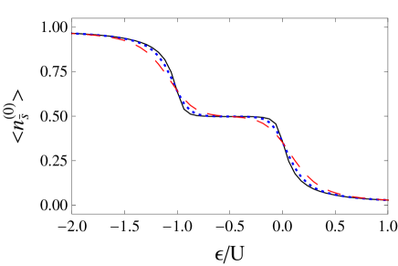
Figure 2: Equilibrium quantum dot occupation number $\langle n_{\bar{s}}^{(0)}\rangle$ as a function of the level position $\varepsilon$ for three values of the temperature: $k_{B}T/U=0.01$ (full black curve), $k_{B}T/U=0.05$ (dotted blue curve), and $k_{B}T/U=0.1$ (dashed red curve). Here $\Gamma_{0}=0.1\,U$ and the Fermi energy is set to zero, $\varepsilon_{F}=0$.

The first-order correction to the quantum dot occupation number $\langle n^{(1)}_{\bar{s}}\rangle$, also calculated self consistently using Eq. (47), is shown in Fig. 3 as a function of time for several values of $\varepsilon_{0}$. It is important to emphasize that $\langle n^{(1)}_{\bar{s}}\rangle$ is intrinsically a time-dependent quantity and depends on the pumping parameters dynamics, in contrast to $\langle n^{(0)}_{\bar{s}}\rangle$. Notice that the magnitude of $\langle n^{(1)}_{\bar{s}}\rangle$ is typically much smaller than $\langle n^{(0)}_{\bar{s}}\rangle$. We observe that the maximum values of $\langle n^{(1)}_{\bar{s}}\rangle$ occur for $\varepsilon_{0}=\varepsilon_{F}$. When the position of the level $\varepsilon_{0}$ deviates significantly from $\varepsilon_{F}$, charge pumping is attenuated and the magnitude of the current is smaller.

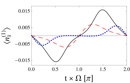
Figure 3: First-order correction to the quantum dot occupation number, $\langle n^{(1)}_{\bar{s}}\rangle$, as a function of time over a complete pumping cycle for three values of $\varepsilon_{0}$: $\varepsilon_{0}/U=-0.075$ (dotted blue curve), $\varepsilon_{0}/U=0$ (full black curve), and $\varepsilon_{0}/U=0.075$ (dashed red curve). Temperature is $k_{B}T/U=0.01$, $\phi_{L}=-\phi_{R}=\pi/2$, $\varepsilon_{1}/U=0.05$, $\Gamma_{0}/U=0.1$, and $\Delta\Gamma/U=0.05$.

After computing $\langle n^{(1)}_{\bar{s}}\rangle$, the next step is to calculate the first-order correction to the time-dependent current $J^{(1)}_{\alpha}(t)$ given by the sum of the fluctuation term $J^{(1){\rm fl}}_{\alpha}(t)$, Eq. (53), and the dissipation terms $J^{(1a){\rm dis}}_{\alpha}(t)$ and $J^{(1b){\rm dis}}_{\alpha}(t)$, Eqs. (55) and (56), respectively. A typical result is shown in Fig. 4 where we plot the frequency independent quantity $J^{(1)}_{\alpha}/\Omega$ as a function of time over a full pumping cycle. It is important to point out that the second dissipation term, $J^{(1b){\rm dis}}_{\alpha s}(t)$, does not contribute to the total charge pumped per cycle since it is proportional to a total time derivative. Consequently, its time integral over a complete pumping cycle must vanish, a result that has been confirmed numerically. The analysis of Fig. 4 reveals that these three current terms, as $\langle n^{(1)}_{\bar{s}}\rangle$, exhibit maxima precisely at the instants when the resonance energy level $\varepsilon(t)$ crosses the Fermi energy. In the case of Fig. 4, where $\varepsilon_{0}=0$, these maxima occur at $t=\pi/2\Omega$ and $t=3\pi/2\Omega$.

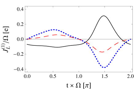
Figure 4: The three terms that contribute to the first-order correction to the pumping current as a function of time: $J^{(1){\rm fl}}_{\alpha}(t)$ (dotted blue curve), $J^{(1a){\rm dis}}_{\alpha}(t)$ (dashed red curve), and $J^{(1b){\rm dis}}_{\alpha}(t)$ (full black curve). Here we set $\varepsilon_{0}=0$ and take the other model parameters as in Fig. 3.

There is an intuitive interpretation for the role of the pumping parameters of our model, $\Gamma_{R,L}(t)$ and $\varepsilon(t)$, that helps us to understand the time dependence observed above: In Eq. (59) we fixed the phase offset of $\varepsilon(t)$ to zero. In this situation, for $0\leq t\leq\tau_{\rm pump}/2$ the resonance energy $\varepsilon$ decreases with time. As a consequence, during this half pumping period $\langle n_{s}\rangle$ increases with time, which corresponds to loading negative charge into the quantum dot. In this time interval, the sign of the pumping current depends on the phase difference between $\phi_{R}$ and $\phi_{L}$. The situation is reversed for $\tau_{\rm pump}/2\leq t\leq\tau_{\rm pump}$. Figure 5 shows the three-dimensional plot of the charge pumped per cycle $Q$ as a function of both $\phi_{R}$ and $\phi_{L}$. Consistent with the reasoning presented above, having $\phi_{L}$ and $\phi_{R}$ in anti-phase favors larger values of $|Q|$. In particular, we find two maximum values of $|Q|$, one at $\phi_{L}=\pi/2$ and $\phi_{R}=3\pi/2$, and the other at $\phi_{L}=-\pi/2$ and $\phi_{R}=\pi/2$. The location of these maxima shows no dependence on any of the model parameters, provided $\varepsilon_{1}\neq 0$. In this limit case, there are only two active pumping parameters, $\Gamma_{R}$ and $\Gamma_{L}$, and the dependence of $Q$ on the $\phi_{R}$ and $\phi_{L}$ is the same as in the non-interacting case.brouwer98 Since we are interested in maximizing $|Q|$, in the remaining of this paper we take $\varepsilon_{1}\neq 0$ and $\phi_{L}=-\phi_{R}=\pi/2$.

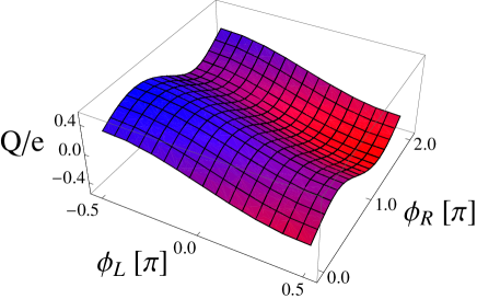
Figure 5: Three-dimensional graph of $Q$ as a function of $\phi_{L}$ and $\phi_{R}$. Temperature is $k_{B}T/U=0.01$ while $\varepsilon_{0}=0$, $\varepsilon_{1}/U=0.05$, $\Gamma_{0}/U=0.1$, and $\Delta\Gamma/U=0.05$.

We are now ready to study the dependence of $Q$ on $V_{g}(t)$, related to $\varepsilon_{0}$ and $\varepsilon_{1}$, as well as on the dot-lead couplings, represented in our model by $\Gamma_{0}$ and $\Delta\Gamma$.

In Fig. 6 we show the charge pumped per cycle $Q$ calculated as a function of $\varepsilon_{0}$. Charge pumping is enhanced whenever a quantum dot resonance, $\varepsilon_{0}$ or $\varepsilon_{0}+U$, crosses the Fermi level, resulting in the two peaks of Fig. 6.

Figure 6: Charge pumped per cycle as a function of the level position $\varepsilon_{0}$ for $\varepsilon_{1}/U=0.05$, $k_{B}T/U=0.01$, $\phi_{L}=-\phi_{R}=\pi/2$, $\Gamma_{0}/U=0.1$, and $\Delta\Gamma/U=0.05$. The charge is measured in units of the electron charge $e$.

Figure 7 shows the dependence of $Q$ on $\varepsilon_{1}$. We consider one of the situations of maximum pumping, namely, $\phi_{L}=-\phi_{R}=\pi/2$ and $\varepsilon_{0}=\varepsilon_{F}=0$. In this case, $|Q|$ increases monotonically with $\varepsilon_{1}$. We caution that once $\varepsilon_{1}$ exceeds $\Gamma_{0}$, it is necessary to check whether $\xi\ll 1$, so that the adiabatic approximation still holds. Hence, increasing $\varepsilon_{1}$ might not be advantageous whenever it is necessary to reduce $\Omega$. Figure 7 also shows that $Q$ vanishes when $\varepsilon_{1}$= 0, as expected for a two-parameter adiabatic pump that occur for $\phi_{L}=-\phi_{R}=\pi/2$.thouless ; brouwer98

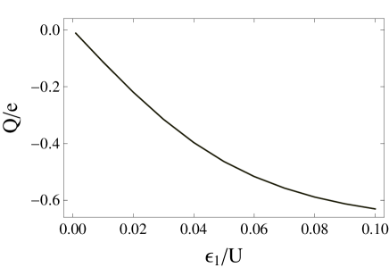
Figure 7: Charge pumped per cycle as a function of the resonance oscillation amplitude $\varepsilon_{1}$ for $\varepsilon_{0}=0$, $\Gamma_{0}/U=0.1$, $\Delta\Gamma/U=0.05$, $k_{B}T/U=0.01$, and $\phi_{L}=-\phi_{R}=\pi/2$. The charge is measured in units of the electron charge $e$.

We now address the dependence of $Q$ on $\Delta\Gamma$ and $\Gamma_{0}$. To be quantitative, we now also keep $T\gg T_{K}$ for the sake of the validity of our approximation. To maximize pumping, we find that it is advantageous to decrease $T_{K}$ by taking $\varepsilon_{0}\neq 0$ rather than increasing $T$. As before, we consider $\phi_{L}=-\phi_{R}=\pi/2$. Due to the time derivatives appearing in the Green’s function expressions, several terms in Eqs. (53) and (55) are proportional to $\Delta\Gamma$. Indeed, we find that $Q$ is roughly linear in $\Delta\Gamma$ for several values of $\varepsilon_{1}\leq\Gamma_{0}$. Figure 8 shows $Q$ versus $\Gamma_{0}$ for three temperature values. Due to the fact that $k_{B}T_{K}\leq\sqrt{\Gamma U/2}e^{-\pi/2}$ for $\varepsilon\approx\Gamma_{0}$, our approximation scheme breaks down as $\Gamma_{0}$ is increased and $T_{K}$ reaches $T$.

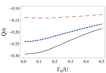
Figure 8: Charge pumped per cycle as a function of $\Gamma_{0}$ for different values of temperature: $k_{B}T/U=0.05$ (full black curve), $k_{B}T/U=0.1$ (dotted blue curve), and $k_{B}T/U=0.2$ (dashed red curve). Here $\varepsilon_{0}=\Gamma$, $\varepsilon_{1}/U=0.05$, $\Delta\Gamma/\Gamma_{0}=1$, and $\phi_{L}=-\phi_{R}=\pi/2$.

Figure 9 shows $Q$ as a function of temperature for three values of the resonance energy $\varepsilon_{0}$ with $\varepsilon_{1}$ kept fixed. The temperatures for which we observe the largest values of $|Q|$ scale with $\varepsilon_{0}$. We also find that by decreasing $|\varepsilon_{0}|$ the maximum of $|Q|$ increases. Unfortunately, since our results are only valid for $T\gg T_{K}$, we cannot freely vary $\varepsilon_{0}$.

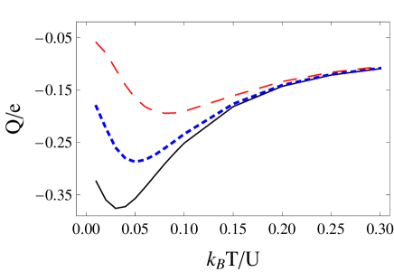
Figure 9: Charge pumped per cycle as a function of temperature for $\varepsilon_{0}/U=0.075$ (full black curve), $\varepsilon_{0}/U=0.1$ (dotted blue curve), and $\varepsilon_{0}/U=0.15$ (dashed red curve). For all curves $\varepsilon_{1}/U=0.05$, $\Gamma_{0}/U=0.1$, $\Delta\Gamma/U=0.1$, and $\phi_{L}=-\phi_{R}=\pi/2$.

Finally, let us address the dependence of $Q$ on the charging energy $U$. Our results are summarized in Fig. 10. A large interval range for $U$ is displayed to best illustrate the pumped charge dependence on this parameter. We observe that pumping is largely enhanced for small values of $U$. When $U$ becomes comparable to $\Gamma$ the system departs from the Coulomb blockade regime.

Figure 10: Charge pumped per cycle as a function of $U/\Gamma_{0}$ for $\varepsilon_{0}=\Gamma_{0}$, $\varepsilon_{1}=\Gamma_{0}/2$, and $k_{B}T=\Delta\Gamma=\Gamma_{0}$.

VI Conclusions

In conclusion, we have investigated adiabatic charge pumping through quantum dots in the Coulomb blockade regime. We specifically studied the impact of Coulomb interaction on the pumping current amplitude for the finite-U Anderson model, in contrast to previous works that treated the infinite-$U$ case.Splettstoesser05

We have derived a general expression for the adiabatic pumping current that is proportional to the instantaneous Green’s function of the dot. This formula was then applied to compute the time dependence of the total charge pumped per cycle through the dot. This allowed us to analyze several aspects of experimental relevance, such as the dependence of the pumped charge on temperature and on the phase difference between time-dependent perturbations.

We find that, within the adiabatic regime, there is a large range of parameters that can be used to maximize the charge pumped per cycle. For this purpose, we find that it is advantageous to: (i) Tune the back gate voltage to pump with the QD in resonance with the Fermi energy in the leads; (ii) maximize the pumping amplitude $\Delta\Gamma$ and, possibly, $\varepsilon_{1}$ as well; (iii) minimize temperature.

We were not able to find a set of parameter values that gives one unit of charge $e$ per pumping cycle within the parameter ranges allowed by our approximations. We do not discard such interesting possibility, but our investigations hint that it may only be possible for very particular pulse formats, not necessarily sinusoidal, and within a narrow parameter interval. The possibility of spin pumping and the consideration of the double-dot case are under investigation and will be reported soon.

References

- (1) D. J. Thouless, Phys. Rev. B 27, 6083 (1983).
- (2) P. W. Brouwer, Phys. Rev. B 58, R10135 (1998).
- (3) M. Büttiker, H. Thomas, and A. Prêtre, Z. Phys. B 94, 133 (1994).
- (4) I. L. Aleiner, B. L. Altshuler, and A. Kamenev, Phys. Rev. B 62, 10373 (2000).
- (5) M. Moskalets and M. Büttiker, Phys. Rev. B 64, 201305(R) (2001).
- (6) J. N. H. J. Cremers and P. W. Brouwer, Phys. Rev. B 65, 115333 (2002).
- (7) M. Moskalets and M. Büttiker, Phys. Rev. B 66, 035306 (2002).
- (8) F. Taddei, M. Governale, and R. Fazio, Phys. Rev. B 70, 052510 (2004).
- (9) M. Blaauboer, Phys. Rev. B 65, 235318 (2002).
- (10) E. R. Mucciolo, C. Chamon, and C. M. Marcus, Phys. Rev. Lett. 89, 146802 (2002).
- (11) M. Martinez-Mares, C. H. Lewenkopf, and E. R. Mucciolo, Phys. Rev. B 69, 085301 (2004).
- (12) E. R. Mucciolo and C. H. Lewenkopf, Int. J. Nanotechnol. 4, 482 (2007).
- (13) M. Governale, F. Taddei and R. Fazio, Phys. Rev. B 68, 155324 (2003).
- (14) O. Entin-Wohlman, A. Aharony, and Y. Levinson, Phys. Rev, B 65, 195411 (2002).
- (15) M. G. Vavilov, V. Ambegaokar, and I. L. Aleiner, Phys. Rev. B 63, 195313 (2001).
- (16) H. Pothier, P. Lafarge, C. Urbina, D. Esteve, and M. H. Devoret, Europhysics Lett. 17, 249 (1992).
- (17) M. Switkes, C. M. Marcus, K. Chapman, and A. C. Gossard, Science 283, 1905 (1999).
- (18) P. J. Leek, M. R. Buitelaar, V. I. Talyanskii, C. G. Smith, D. Anderson, G. A. C. Jones, J. Wei, and D. H. Cobden, Phys. Rev. Lett. 95, 256802 (2005).
- (19) M. R. Buitelaar et al., Phys. Rev. Lett. 101, 126803 (2008).
- (20) B. Kaestner et al., Appl. Phys. Lett. 92, 192106 (2008); B. Kaestner et al., Phys. Rev. B 77, 153301 (2008).
- (21) S. K. Watson, R. M. Potok, C. M. Marcus, and V. Umansky, Phys. Rev. Lett. 91, 258301 (2003).
- (22) T. Aono, Phys. Rev. Lett. 93, 116601 (2004).
- (23) A. Schiller and A. Silva, Phys. Rev. B 77, 045330 (2008).
- (24) L. Arrachea, A. Levy Yeyati, and A. Martin-Rodero, Phys. Rev. B 77, 165326 (2008).
- (25) P. W. Brouwer, A. Lamacraft, and K. Flensberg, Phys. Rev. B 72, 075316 (2005).
- (26) E. Cota, R. Aguado, and G. Platero, Phys. Rev. Lett. 94, 107202 (2005).
- (27) I. L. Aleiner and A. V. Andreev, Phys. Rev. Lett. 81, 1286 (1998).
- (28) J. Splettstoesser, M. Governale, J. König, and R. Fazio, Phys. Rev. Lett. 95, 246803 (2005).
- (29) E. Sela and Y. Oreg, Phys. Rev. Lett. 96, 166802 (2006).
- (30) J. Splettstoesser, M. Governale, J. König, and R. Fazio, Phys. Rev. B 74, 085305 (2006).
- (31) P. Devillard, V. Gasparian, and T. Martin, Phys. Rev. B 78, 085130 (2008).
- (32) D. Fioretto and A. Silva, Phys. Rev. Lett. 100, 236803 (2008).
- (33) M. Braun and G. Burkard, Phys. Rev. Lett. 101, 036802 (2008).
- (34) F. Cavaliere, M. Governale, J. König, arXiv:0904.1687 (2009).
- (35) J. Rammer and H. Smith, Rev. Mod. Phys. 58, 323 (1986).
- (36) H. Haug and A.-P. Jauho, Quantum Kinetics in Transport and Optics of Semiconductors (Springer-Verlag, Heidelberg, 1996).
- (37) A.-P. Jauho, N. S. Wingreen, and Y. Meir, Phys. Rev. B 50, 5528 (1994).
- (38) A. C. Hewson, The Kondo Problem to Heavy Fermions (Cambridge University Press, Cambridge, England, 1993).
- (39) Y. Meir, N. S. Wingreen, and P. A. Lee, Phys. Rev. Lett. 66, 3048 (1991).
- (40) D. C. Langreth, Phys. Rev. 148, 707 (1966).
- (41) A. Hernández, V. M. Apel, F. A. Pinheiro, and C. H. Lewenkopf, Physica A 385, 148 (2007).
- (42) Although this demonstration has been made for the retarded component, it also applies for the lesser and greater ones.
- (43) N. Winkler, M. Governale, and J. König, Phys. Rev. B 79, 235309 (2009).