Genuine tripartite entanglement in quantum brachistochrone evolution of a three-qubit system

Abstract

We explore the connection between quantum brachistochrone (time-optimal) evolution of a three-qubit system and its residual entanglement called three-tangle. The result shows that the entanglement between two qubits is not required for some brachistochrone evolutions of a three-qubit system. However, the evolution between two distinct states cannot be implemented without its three-tangle, except for the trivial cases in which less than three qubits attend evolution. Although both the probability density function of the time-averaged three-tangle and that of the time-averaged squared concurrence between two subsystems become more and more uniform with the decrease in angles of separation between an initial state and a final state, the features of their most probable values exhibit a different trend.

I introduction

The speed of the evolution of a quantum system governed by a given energy constraint is very important in quantum information as it provides a useful tool for people to estimate the fundamental limits that basic physical laws impose on how fast information can be processed or transmitted Margolus ; Levitin ; Zielinski ; Kosinski . Also, one can exploit the limit on the speed of quantum evolution to construct an optimal quantum gate with which the quantum time required for a system to evolve between two mutually orthogonal states is the shortest one bgate . However, two elementary relations limit the speed of quantum evolution. On the one hand, the time-energy uncertainty relation Anandan imposes a lower limit on the time interval $T$ taken by a quantum system to evolve from a given state to its orthogonal one. This bound on $T$ is related to the spread of energy of the system $\triangle E$, i.e., $T\geq\frac{h}{4\triangle E}$. On the other hand, Margolus and Levitin Margolus showed that such a quantity is also related to the fixed average energy of the system $E$, i.e., $T\geq\frac{h}{4E}$. These two relations together establish the limit time of quantum evolution speed, i.e., the minimum time $T(E,\triangle E)$ required for a system with the energy $E$ and the energy spread $\triangle E$ to evolve through two orthogonal states. Recently, Giovannetti, Lloyd and Maccone Giovannetti ; Giovannettipra ; GiovannettiJOB showed that there is an interesting connection between quantum entanglement and the evolution speed of quantum systems. Some groups Giovannetti ; Giovannettipra ; GiovannettiJOB ; Kupferman have studied the connection between entanglement and the speed of evolution in mixed states. This connection has been extensively studied for the evolution between orthogonal and nonorthogonal, pure and mixed, as well as bipartite and multipartite cases add1 ; add2 ; add3 ; add4 ; BorrasZander ; Borras .

Quantum brachistochrone evolution problem is used to deal with the Hamiltonian generating the optimal quantum evolution $|\psi(t)\rangle$ between two prescribed states $|\psi_{I}\rangle$ and $|\psi_{F}\rangle$ qbepprl . That is, it searches the shortest time interval $T$ taken by a quantum system for evolving from an original state to a final one. This problem attracts a lot of attention qbepprl ; qbep2 ; CarliniHosoya . For instance, Carlini et al. qbepprl presented a general framework for finding the time-optimal evolution and the optimal Hamiltonian for quantum system with a given set of initial and final states. Brody and Hook qbep2 established an elementary derivation of the optimum Hamiltonian, under constraints on its eigenvalues, that generates the unitary transformation $|\psi_{I}\rangle\rightarrow|\psi_{F}\rangle$ in the shortest duration. Carlini et al. CarliniHosoya investigated quantum brachistochrone evolution of mixed states.

Recently, Borras et al. BorrasZander investigated the role of entanglement in quantum brachistochrone evolution of quantum system in a pure state and found that ” brachistochrone quantum evolution between orthogonal states cannot be implemented without entanglement”. Moreover, they Borras discussed quantum brachistochrone evolution of systems of two identical particles and found that entanglement plays a fundamental role in the brachistochrone evolution of composite quantum systems. That is, quantum brachistochrone evolution of a composite quantum systems composed of distinguishable subsystems cannot be implemented without entanglement if there are at least two subsystems attending evolutions. In these two works BorrasZander ; Borras , they gave out the connection between the entanglement of two subsystems (i.e., the linear entropy of two subsystems BorrasZander or their squared concurrence C² Borras ) and time-optimal quantum evolutions in the cases of two-qubit systems, two-qutrit systems and three-qubit systems.

In three-qubit systems, there is another entanglement shared by all the three qubits, i.e., the so-called residual entanglement by Coffman, Kundu, and Wootters CKW . It is termed as three-tangle $\tau_{ABC}$ threetangle and can be expressed as CKW

$$\tau_{ABC}=C^{2}_{A(BC)}-C^{2}_{AB}-C^{2}_{AC},$$ (1)

where $C_{A(BC)}$ is the concurrence of the two subsystems $A$ and $BC$. In detail, concurrence is a useful tool for quantifying the entanglement of bipartite quantum systems and it is given by wotters

$$C_{AB}=max\{0,\lambda_{1}-\lambda_{2}-\lambda_{3}-\lambda_{4}\},$$ (2)

where $\lambda_{1}\geq\lambda_{2}\geq\lambda_{3}\geq\lambda_{4}$ are the square roots of the eigenvalues of the matrix $\rho_{AB}(\sigma^{A}_{y}\otimes\sigma^{B}_{y})\rho^{*}_{AB}(\sigma^{A}_{y}\otimes\sigma^{B}_{y})$. Here $\rho_{AB}$ is the matrix of the bipartite quantum system $AB$ and $\rho^{*}_{AB}$ is its complex conjugation. $\sigma^{A}_{y}$ is the Pauli matrix expressed in the same basis as

$$\sigma_{y}=\left(\begin{array}[]{cc}0&-i\\ i&0\end{array}\right).$$ (5)

Different from concurrence $C_{A(BC)}$ which is shared only by two subsystems $A$ and $BC$, $\tau_{ABC}$ is real entanglement shared among the three particles of the system. That is, it is invariant under permutations of the three qubits, i.e., $\tau_{ABC}=\tau_{BCA}=\tau_{CAB}$.

In this paper, we will explore the connection between three-tangle $\tau_{ABC}$ and quantum brachistochrone evolution of a three-qubit system. Our result shows that in some special cases of quantum brachistochrone evolution of a three-qubit system, the entanglement between two subsystems $C^{2}_{AB}$ ($C^{2}_{AC}$) is not required. However, the evolution between two distinct states cannot be implemented without three-tangle $\tau$, except for the trivial cases in which there are less than three qubits attending quantum brachistochrone evolution. Our result is tighter than that in Ref.BorrasZander for quantum brachistochrone evolution of a three-qubit system. Moreover, we find that both the probability density function of the time-averaged three-tangle and that of the time-averaged squared concurrence between two subsystems become more and more uniform with the decrease in angles of separation between an initial state and a final state, but the features of their most probable values exhibit a different trend.

The paper is organized as follows. In Sec. II A, we describe the way for the calculation of time averaged three-tangle in quantum brachistochrone evolution. In Sec. II B, we discuss the role of three-tangle $\tau_{ABC}$ in quantum brachistochrone evolution and find that brachistochrone evolutions cannot be implemented without $\tau_{ABC}$. However, the entanglement of each two qubits is not necessary in some brachistochrone evolutions. In Secs. III A and III B, we give the probability density of $\langle\tau\rangle$ in quantum brachistochrone evolutions between two symmetric states with the different angles of separation ($\theta/2=\pi/8,\pi/4,3\pi/8,\pi/2$) and that between two general states, respectively. A brief discussion and summary are given in Sec. IV.

II time averaged entanglement during brachistochrone evolution

II.1 Time averaged three-tangle in quantum brachistochrone evolution

Quantum brachistochrone evolution problem means searching the shortest possible time for generating the optimal quantum evolution $|\psi(t)\rangle$ from an initial quantum state $|\Psi_{I}\rangle$ to a final quantum state $|\Psi_{F}\rangle$ under the constraint that the difference between the maximum eigenenergy and the minimum one of the Hamiltonians $H_{T}$ generating the unitary transformation $|\Psi_{I}\rangle\rightarrow|\Psi_{F}\rangle=e^{\frac{iH_{T}}{\hbar}}|\Psi_{I}\rangle$ is not more than a given constant energy 2$\omega$. This constraint is necessary as it is easy to implement a quantum evolution connecting the two alluded states and taking an arbitrarily small time $T$ if the differences between the eigenenergies of the Hamiltonians are arbitrarily large BorrasZander . The time-optimal evolution is given by qbepprl ; qbep2 ; BorrasZander

$$|\Psi(t)\rangle=[\text{cos}(\frac{\omega t}{\hbar})-\frac{\text{cos}\frac{1}{2}\theta}{\text{sin}\frac{1}{2}\theta}\text{sin}(\frac{\omega t}{\hbar})]|\Psi_{I}\rangle$$

$$+\frac{1}{\text{sin}\frac{1}{2}\theta}\text{sin}(\frac{\omega t}{\hbar})|\Psi_{F}\rangle.$$ (6)

Here $|\psi(0)\rangle=|\Psi_{I}\rangle$ and $|\psi(T)\rangle=|\Psi_{F}\rangle$ represent the initial state and the final one, respectively, and

$$T=\frac{\hbar\theta}{2\omega}.$$ (7)

$\theta$ can be regarded as the angle of separation of the initial and the final states. If this pair of states are orthogonal, i.e., $\langle\Psi_{I}|\Psi_{F}\rangle=0$ ($\theta=\pi$), then

$$T = \frac{\pi\hbar}{2\omega},$$ (8)

$$|\Psi(t)\rangle = \text{cos}(\frac{\omega t}{\hbar})|\Psi_{I}\rangle+\text{sin}(\frac{\omega t}{\hbar})|\Psi_{F}\rangle.$$ (9)

During the time-optimal evolution, the time averaged three-tangle can be calculated as follows

$$\langle\tau(\Psi(t))\rangle = \frac{1}{T}\int_{0}^{T}\tau(\Psi(t))dt,$$ (10)

where $\tau(\Psi(t))$ is the three-tangle of a three-qubit system in the state $\Psi_{ABC}(t)$. For an arbitrary three-qubit pure state

$$|\Psi\rangle_{ABC}=\sum a_{ijk}|ijk\rangle_{ABC},\;\;\;\;(i,j,k\in\{0,1\}),$$ (11)

its three-tangle $\tau_{ABC}(\Psi)$ can be calculated as follows: CKW

$$\tau_{ABC}(\Psi)=4|d_{1}-2d_{2}+4d_{3}|,$$ (12)

where

$$d_{1} = a_{000}^{2}a_{111}^{2}+a_{001}^{2}a_{110}^{2}+a_{010}^{2}a_{101}^{2}+a_{100}^{2}a_{011}^{2},$$

$$d_{2} = a_{000}a_{111}a_{100}a_{011}+a_{000}a_{111}a_{101}a_{010}$$

$$+ a_{000}a_{111}a_{110}a_{001}+a_{011}a_{100}a_{101}a_{010}$$

$$+ a_{011}a_{100}a_{110}a_{001}+a_{010}a_{101}a_{110}a_{001},$$

$$d_{3} = a_{000}a_{110}a_{101}a_{011}+a_{111}a_{001}a_{010}a_{100}.$$ (13)

For example, the three-tangle $\tau$ in a standard Greenberger-Horne-Zeilinger (GHZ) state $|GHZ\rangle=\frac{1}{\sqrt{2}}(|000\rangle+|111\rangle)$ is 1 and that in a W state $|W\rangle=\frac{1}{\sqrt{3}}(|001\rangle+|010\rangle+|100\rangle)$ is 0.

II.2 Role of three-tangle in quantum brachistochrone evolution

Borras et al. BorrasZander ; Borras showed that quantum brachistochrone evolution between orthogonal states cannot be implemented without the typical entanglement of two subsystems (such as linear entropy or concurrence). For a three-qubit entangled quantum system, its concurrence satisfies the following relation,

$$C^{2}_{A(BC)}=C^{2}_{AB}+C^{2}_{AC}+\tau_{ABC}.$$ (14)

That is, $C^{2}_{A(BC)}$ includes three parts. Our question is, is each term of the three parts in $C^{2}_{A(BC)}$ necessary in a quantum brachistochrone evolution?

Let us consider two specific cases of time-optimal evolution of three-qubit symmetric states with the following two pairs of initial and final states to analyze the role of the three terms $C^{2}_{AB}$, $C^{2}_{AC}$, and $\tau_{ABC}$.

$$(i)\;\;|\Psi^{1}_{I}\rangle = \frac{1}{\sqrt{3}}(|110\rangle+|101\rangle+|011\rangle)\rightarrow|\Psi^{1}_{F}\rangle$$ (15)

$$= \frac{\text{cos}\alpha}{\sqrt{2}}(|000\rangle+|111\rangle)+\frac{\text{sin}\alpha}{\sqrt{3}}(|001\rangle$$

$$+ |010\rangle+|100\rangle),$$

$$(ii)\;\;|\Psi^{2}_{I}\rangle = \frac{1}{\sqrt{2}}(|000\rangle-i|111\rangle)\rightarrow|\Psi^{2}_{F}\rangle$$ (16)

$$= \frac{1}{\sqrt{2}}(i|000\rangle-|111\rangle).$$

Here $\langle\Psi^{j}_{I}|\Psi^{j}_{F}\rangle=0$ ($j=1,2$).

In the case ($i$), the three-tangle $\tau_{ABC}$ in the initial state $|\Psi^{1}_{I}\rangle$ is 0. The final state $|\Psi^{1}_{F}\rangle$ is a superposition of $|GHZ\rangle$ and $|W\rangle$ and its three-tangle is determined by the coefficient $\alpha$. When $\alpha=0$ the final state is a $|GHZ\rangle$ state and its three-tangle is 1. When $\alpha=\frac{\pi}{2}$ the final state is a $|W\rangle$ state and its three-tangle is 0. During the time-optimal evolution, the state of the three-qubit system $ABC$ at the time $t$ is described by Eq.(9). Let $\xi=\frac{\omega t}{\hbar}$, the state can be written as

$$|\Psi(\xi,\alpha)\rangle_{ABC} = \text{cos}\xi\frac{1}{\sqrt{3}}(|110\rangle+|101\rangle+|011\rangle)_{ABC}$$

$$+ \text{sin}\xi[\frac{\text{cos}\alpha}{\sqrt{2}}(|000\rangle+|111\rangle)_{ABC}$$

$$+ \frac{\text{sin}\alpha}{\sqrt{3}}(|100\rangle+|010\rangle+|001\rangle)_{ABC}].$$

The three-tangle in the state $|\Psi(\xi,\alpha)\rangle_{ABC}$ is given by

$$\tau(\xi,\alpha)_{ABC} = 4|\frac{1}{4}\text{sin}^{4}\xi\text{cos}^{4}\alpha-\frac{1}{3}\text{sin}^{2}\xi\text{cos}^{2}\xi\text{sin}^{2}\alpha$$ (18)

$$-\text{sin}^{3}\xi\text{cos}\xi\text{sin}\alpha\text{cos}^{2}\alpha$$

$$+\frac{4}{3\sqrt{6}}\text{sin}\xi\text{cos}^{3}\xi\text{cos}\alpha$$

$$+\frac{4}{3\sqrt{6}}\text{sin}^{4}\xi\text{sin}^{3}\alpha cos\alpha|.$$

The time average three-tangle can be calculated by

$$\langle\tau(\alpha)\rangle_{ABC} = \frac{2}{\pi}\int_{0}^{\frac{\pi}{2}}\tau(\xi,\alpha)_{ABC}d\xi.$$ (19)

Figure 1: Plot of $\langle\tau(\alpha)\rangle$ as a function of $\alpha$ ($\alpha\in[0,\frac{\pi}{2}]$) for the time-optimal evolutions from $|\Psi_{I}\rangle_{1}$ to $|\Psi_{F}\rangle_{1}$.

The relation between the time averaged three-tangle $\langle\tau(\alpha)\rangle$ and the parameter $\alpha$ is shown in Fig.1. For $|\Psi^{1}_{I}\rangle=|\widetilde{W}\rangle=\frac{1}{\sqrt{3}}(|110\rangle+|101\rangle+|011\rangle)\rightarrow|\Psi^{1}_{F}\rangle=|GHZ\rangle=\frac{1}{\sqrt{2}}(|000\rangle+|111\rangle)$ ($\alpha=0$), $\langle\tau(0)\rangle=0.7215$; for $|\Psi^{1}_{I}\rangle=\frac{1}{\sqrt{3}}(|110\rangle+|101\rangle+|011\rangle)\rightarrow|\Psi^{1}_{F}\rangle=\frac{1}{\sqrt{3}}(|001\rangle+|010\rangle+|100\rangle)$ ($\alpha=\pi/2$), $\langle\tau(\pi/2)\rangle=0.1667$. From Fig.1, one can see that the time averaged three-tangle is maximal when the three-qubit quantum system evolves from the state $|\widetilde{W}\rangle=\frac{1}{\sqrt{3}}(|110\rangle+|101\rangle+|011\rangle)$ to the state $|GHZ\rangle=\frac{1}{\sqrt{2}}(|000\rangle+|111\rangle)$. Moreover, the time averaged three-tangle is larger than zero, which means the three-tangle $\tau_{ABC}=1$ is necessary in these evolutions.

In the case ($ii$), the state of the three-qubit system at the time $t$ is

$$|\Psi(t)\rangle=\frac{1}{\sqrt{2}}(e^{i\frac{\omega t}{\hbar}}|000\rangle-ie^{-i\frac{\omega t}{\hbar}}|111\rangle).$$ (20)

The three-tangle of the three-qubit system during the time-optimal evolution is $\tau_{ABC}=C^{2}_{A(BC)}=1$, i.e., $C^{2}_{AB}=C^{2}_{AC}=0$, which means the entanglement of each two qubits $C_{AB}$ ($C_{AC}$ or $C_{BC}$) is not required in this time-optimal evolution. However, it requires the three-tangle $\tau_{ABC}$. In other words, this time-optimal evolution cannot be implemented without the three-tangle $\tau_{ABC}$.

Certainly, there is at least a class of initial states and final states making the three-tangle be $\tau_{ABC}=C^{2}_{A(BC)}=1$ during the time-optimal evolution. That is, the initial state is

$$|\Psi^{2^{\prime}}_{I}\rangle=\frac{1}{\sqrt{2}}(e^{i\phi_{A}}|klm\rangle-e^{i\phi_{B}}|\bar{k}\bar{l}\bar{m}\rangle),$$ (21)

the final state is

$$|\Psi^{2^{\prime}}_{F}\rangle=\frac{i}{\sqrt{2}}(e^{i\phi_{A}}|klm\rangle+e^{i\phi_{B}}|\bar{k}\bar{l}\bar{m}\rangle),$$ (22)

and the state at the time $t$ during the time-optimal evolution is

$$|\Psi^{\prime}(t)\rangle=\frac{1}{\sqrt{2}}(e^{i\frac{\omega t}{\hbar}+i\phi_{A}}|klm\rangle-e^{-i\frac{\omega t}{\hbar}+i\phi_{B}}|\bar{k}\bar{l}\bar{m}\rangle).$$ (23)

Here $\phi_{A}$ and $\phi_{B}$ are two arbitrary real numbers. $k,l,m\in\{0,1\}$ and $\bar{k}=1-k$.

From these two special cases of time-optimal evolutions of three-qubit symmetric states, one can see that the entanglement of each two qubits $C_{AB}$ ($C_{AC}$ or $C_{BC}$) is not necessary in some brachistochrone evolutions. However, the brachistochrone evolutions cannot be implemented without the three-tangle $\tau$.

III three-tangle in quantum brachistochrone evolution

III.1 Three-tangle in quantum brachistochrone evolution between two symmetric states

In order to explore the typical features of $\langle\tau\rangle$ in all possible brachistochrone evolutions of a three-qubit system $ABC$ between a pair of symmetric states, we are going to sample systematically the aforementioned set of time-optimal evolutions by generating randomly pairs of symmetric states $|\Psi_{I}\rangle_{ABC}$ and $|\Psi_{F}\rangle_{ABC}$ with a given overlap $\langle\Psi_{I}|\Psi_{F}\rangle=cos(\theta/2)$, i.e.,

$$|\Psi_{I}\rangle_{ABC}=c_{1}|000\rangle+c_{2}\frac{1}{\sqrt{3}}\{|001\rangle+|010\rangle+|100\rangle\}$$

$$+c_{3}\frac{1}{\sqrt{3}}\{|110\rangle+|101\rangle+|011\rangle\}+c_{4}|111\rangle,$$ (24)

$$|\Psi_{F}\rangle_{ABC}=d_{1}|000\rangle+d_{2}\frac{1}{\sqrt{3}}\{|001\rangle+|010\rangle+|100\rangle\}$$

$$+d_{3}\frac{1}{\sqrt{3}}\{|110\rangle+|101\rangle+|011\rangle\}+d_{4}|111\rangle,$$ (25)

where

$$\sum_{k=1}^{4}|c_{k}^{2}| = \sum_{k}^{4}|d_{k}^{2}|=1,$$ (26)

$$\sum_{k=1}^{4}c_{k}d_{k}^{\ast} = cos(\theta/2).$$ (27)

It is easy to see that the three qubits $A$, $B$, and $C$ are symmetric (uniform) in the initial state $|\Psi_{I}\rangle_{ABC}$ and the final state $|\Psi_{F}\rangle_{ABC}$.

We use the same way as Refs.BorrasZander ; Borras to generate randomly these pairs of states. In detail, let us use $|\Psi\rangle=\sum_{k=1}^{4}c_{k}|k\rangle$ to describe a general state of a three-qubit system. Here $\{|k\rangle\}$ ($k=1,2,3,4$) is a set of basis states for the three-qubit system $ABC$, i.e, $\{|k\rangle\}=\{|000\rangle,\frac{1}{\sqrt{3}}\{|001\rangle+|010\rangle+|100\rangle\},\frac{1}{\sqrt{3}}\{|110\rangle+|101\rangle+|011\rangle\},|111\rangle\}$, and $\sum_{k=1}^{4}|c_{k}|^{2}=1$. Each pair of states $|\Psi_{I}\rangle$ and $|\Psi_{F}\rangle$ can be generated with the Haar measure Zyczkowski by random $4\times 4$ unitary matrices $M_{4\times 4}$ uniformly distributed upon the vectors $|\Psi_{I0}\rangle=(1,0,0,0)^{\dagger}$ and $|\Psi_{F0}\rangle=(cos\frac{\theta}{2},sin\frac{\theta}{2},0,0)^{\dagger}$, i.e., $|\Psi_{I}\rangle=M_{4\times 4}|\Psi_{I0}\rangle$ and $|\Psi_{F}\rangle=M_{4\times 4}|\Psi_{F0}\rangle$. For each rotation matrix $M_{4\times 4}$, the pair of symmetric states $|\Psi_{I}\rangle_{ABC}$ and $|\Psi_{F}\rangle_{ABC}$ have an overlap $\langle\Psi_{I}|\Psi_{F}\rangle=cos(\theta/2)$. As the matrix $M_{4\times 4}$ is a random unitary one, the initial state $|\Psi_{I}\rangle$ and the final state $|\Psi_{F}\rangle$ generated by this matrix are a random pair with an overlap $\langle\Psi_{I}|\Psi_{F}\rangle=cos(\theta/2)$. For each of these pairs of states, we calculate the time averaged three-tangle $\langle\tau\rangle$ in the quantum brachistochrone evolution connecting the initial state $|\Psi_{I}\rangle_{ABC}$ and the final state $|\Psi_{F}\rangle_{ABC}$.

The probability densities of $\langle\tau\rangle$ and $P(\langle C^{2}_{A(BC)}\rangle)$ in quantum brachistochrone evolutions between two symmetric states with the different angles of separation ($\theta/2=\pi/8,\pi/4,3\pi/8,\pi/2$) are shown in Fig.2(a) and Fig.2(b), respectively. From this figure, one can see that both $P(\langle\tau\rangle)$ and $P(\langle C^{2}_{A(BC)}\rangle)$ become more uniform when the angle becomes smaller. The smaller the angle $\theta/2$, the larger the most probable values of the time averaged entanglement $\langle C^{2}_{A(BC)}\rangle$. On the contrary, the smaller the angle $\theta/2$, the smaller the most probable values of the time averaged entanglement $\langle\tau\rangle$. Except for the trivial evolution between $|\Psi_{I}\rangle$ and $|\Psi_{F}\rangle=|\Psi_{I}\rangle$, the time-optimal evolution between two symmetric states cannot be implemented without the three-tangle $\tau$.

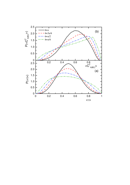
Figure 2: (Color online) (a) Probability density functions $P(\langle\tau\rangle)$ of the three-tangle $\langle\tau\rangle$ corresponding to quantum brachistochrone evolutions of a three-qubit system between two symmetric states with different angles of separation ($\theta/2=\pi/8,\pi/4,3\pi/8,\pi/2$); (b) probability density functions $P(\langle C^{2}_{A(BC)}\rangle)$ of the time averaged squared concurrence $\langle C^{2}_{A(BC)}\rangle$ corresponding to the same evolutions.

III.2 Three-tangle in quantum brachistochrone evolution between two general states

Two general states with a given overlap $cos(\theta/2)$ for a three-qubit system can be described as follows:

$$|\Psi_{I}\rangle = c_{1}|000\rangle+c_{2}|001\rangle+c_{3}|010\rangle+c_{4}|100\rangle$$ (28)

$$+ c_{5}|110\rangle+c_{6}|101\rangle+c_{7}|011\rangle\}+c_{8}|111\rangle,$$

$$|\Psi_{F}\rangle = d_{1}|000\rangle+d_{2}|001\rangle+d_{3}|010\rangle+d_{4}|100\rangle$$ (29)

$$+ d_{5}|110\rangle+d_{6}|101\rangle+d_{7}|011\rangle+d_{8}|111\rangle,$$

where

$$\sum_{k}^{8}|c_{k}|^{2} = \sum_{k}^{8}|d_{k}|^{2}=1,$$ (30)

$$\sum_{k}^{8}c_{k}d_{k}^{\ast} = cos(\theta/2).$$ (31)

Similar to the case with quantum brachistochrone evolution between two symmetric states, we can also calculate the probability density functions $P(\langle\tau\rangle)$ of the time averaged three-tangle $\langle\tau\rangle$ and the probability density functions $P(\langle C^{2}_{A(BC)}\rangle)$ of the time averaged squared concurrence $\langle C^{2}_{A(BC)}\rangle$ corresponding to the same evolutions for $\theta/2=\pi/8,\pi/4,3\pi/8,\pi/2$, shown in Figs.3(a) and 3(b), respectively. From Fig.3, one can get the similar result for the case with two symmetric states in this time.

Compared with the case between two symmetric states, the most probable values of the time averaged entanglement $\langle\tau\rangle$ is smaller with the same angle of separation.

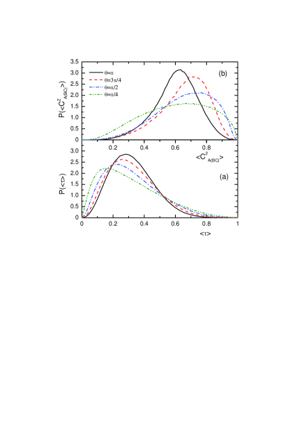
Figure 3: (Color online) (a) Probability density functions $P(\langle\tau\rangle)$ of the three-tangle $\langle\tau\rangle$ corresponding to quantum brachistochrone evolutions of a three-qubit system between two general states with different angles of separation ($\theta/2=\pi/8,\pi/4,3\pi/8,\pi/2$); (b) probability density functions $P(\langle C^{2}_{A(BC)}\rangle)$ of the time averaged squared concurrence $\langle C^{2}_{A(BC)}\rangle$ corresponding to the same evolutions.

IV discussion and summary

There are two classes of trivial evolutions in a three-qubit system. One is the evolution between two same states and the other is that for less than three subsystems. In the first case, the three-qubit system does not evolute as $|\Psi_{I}\rangle=|\Psi(t)\rangle=|\Psi_{F}\rangle$. In the second case, the initial state is $|\Psi_{I}\rangle=|\phi\rangle_{i}\otimes|\psi\rangle_{jk}$ and the final state is $|\Psi_{F}\rangle=|\phi\rangle_{i}\otimes|\psi^{\prime}\rangle_{jk}$ (here $i\neq j\neq k\in\{A,B,C\}$). That is, the qubit $i$ is a stationary particle and it is not correlated with the qubits $j$ and $k$ in the evolution. Similar to the case for the system composed of two identical particles discussed in Ref.Borras , the time-averaged three-tangle required for these trivial quantum brachistochrone evolutions need not be greater than zero. As these evolutions are not genuine three-qubit quantum brachistochrone evolutions, they do not affect our result.

In summary, we have explored the connection between three-tangle and quantum brachistochrone evolution of a three-qubit system. We have shown that the evolution between two distinct states cannot be implemented without three-tangle, except for the trivial cases in which there are less than three qubits attending in quantum brachistochrone evolution or the final state and the initial state are the same one. However, the entanglement between two qubits is not required in some quantum brachistochrone evolutions. Moreover, we have found that both the probability density function of the time-averaged three-tangle $\langle\tau\rangle$ and that of the time-averaged squared concurrence $\langle C^{2}_{A(BC)}\rangle$ between two subsystems become more and more uniform with the decrease in angles of separation $\theta/2$ between an initial state and a final state. However, the features of their most probable values exhibit a different trend. The result between two symmetric states agrees with that between two general states.

References

- (1) N. Margolus and L. B. Levitin, Physica D 120, 188 (1998).
- (2) L. B. Levitin and T. Toffoli, Phys. Rev. Lett. 99, 110502 (2007).
- (3) B. Zielinski and M. Zych, Phys. Rev. A 74, 034301 (2006).
- (4) P. Kosinski and M. Zych, Phys. Rev. A 73, 024303 (2006).
- (5) A. Carlini, A. Hosoya, T. Koike, and Y. Okudaira, Phys. Rev. A 75, 042308 (2007).
- (6) J. Anandan and Y. Aharonov, Phys. Rev. Lett. 65, 1697 (1990).
- (7) V. Giovannetti, S. Lloyd, and L. Maccone, EPL 62, 615 (2003).
- (8) V. Giovannetti, S. Lloyd, and L. Maccone, Phys. Rev. A 67, 052109 (2003).
- (9) V. Giovannetti, S. Lloyd, and L. Maccone, J. Opt. Soc. Am. B 6, S807 (2004).
- (10) J. Kupferman and B. Reznik, Phys. Rev. A 78, 042305 (2008).
- (11) J. Batle, M. Casas, A. Plastino, and A. R. Plastino, Phys. Rev. A 72, 032337 (2005); 73, 049904(E) (2006).
- (12) A. Borras, M. Casas, A. R. Plastino, and A. Plastino, Phys. Rev. A 74, 022326 (2006).
- (13) C. Zander, A. R. Plastino, A. Plastino, and M. Casas, J. Phys. A 40, 2861 (2007).
- (14) V. C. G. Oliveira, H. A. B. Santos, L. A. M. Torres, and A. M. C. Souza, int. J. Quantum Inf. 6, 379 (2008).
- (15) A. Borras, C. Zander, A. R. Plastino, M. Casas, and A. Plastino, Europhys. Lett. 81, 30007 (2008).
- (16) A. Borras, A. R. Plastino, M. Casas, and A. Plastino, Phys. Rev. A 78, 052104 (2008).
- (17) A. Carlini, A. Hosoya, T. Koike, and Y. Okudaira, Phys. Rev. Lett. 96, 060503 (2006).
- (18) D. C. Brody and D. W. Hook, J. Phys. A: Math. Gen. 39, L167 (2006); ibid, 40, 10949 (2007).
- (19) A. Carlini, A. Hosoya, T. Koike and Y. Okudaira, J. Phys. A: Math. Theor. 41, 045303 (2008)
- (20) V. Coffman, J. Kundu, and W. K. Wootters, Phys. Rev. A 61, 052306 (2000).
- (21) A. Wong and N. Christensen, Phys. Rev. A 63, 044301 (2001).
- (22) W. K. Wootters, Phys. Rev. Lett. 80, 2245 (1998).
- (23) I. Bengtsson and K. Życzkowski, Geometry of Quantum States: An Introduction to Quantum Entanglement (Cambridge University Press, Cambridge, 2006); K. Życzkowski and M. Kuś, J. Phys. A: Math. Gen. 27, 4235 (1994).