Proper motions of cool and ultracool candidate members in the Upper Scorpius OB association

Abstract

Aims. Proper motion measurements of the cool and ultracool populations in the Upper Scorpius OB association are crucial to confirm membership and to identify possible run-away objects.

Methods. We cross-match samples of photometrically selected and spectroscopically confirmed cool and ultracool (K5$<$SpT$<$M8.5) candidate members in the Upper Scorpius OB association using the literature and the USNO-B and the UCAC2 catalogues. 251 of these objects have a USNO-B and/or UCAC2 counterpart with proper motion measurements.

Results. A significant fraction (19 objects, 7.6$\pm$1.8%) of spectroscopically confirmed young objects show discrepant proper motion. They must either belong to unidentified coincident foreground associations, or originate from neighboring star forming regions or have recently experienced dynamical interactions within the association. The observed accretor and disc frequencies are lower among outliers, but with only 19 objects it is unreliable to draw firm statistical conclusions. Finally, we note that transverse velocities of very low mass members are indistinguishable from those of low mass members within $\approx$4 km s^-1.

1 Introduction

The galaxy is made of a number of large scale stellar structures such as clusters, star forming regions, and OB associations. Kinematics has been successfully used to identify these associations (e.g Torres et al., 2008; Zuckerman et al., 2004, 2006). The kinematic properties of the different classes of objects in a given association additionally hold important clues about its members history. Some models of formation predict that the early dynamical evolution of the parent proto-stellar cluster should lead to mass-dependent kinematic distributions (Kroupa & Bouvier, 2003) while other numerical simulations predict on the contrary similar kinematic properties over the whole mass spectrum (Bate et al., 2003; Bate, 2009). The kinematic study of low mass stars (LMSs, defined here as objects with spectral type M0$<$SpT$<$K5), very low mass stars (VLMSs, M0$<$SpT$<$M5) and brown dwarfs (BDs, SpT$>$M6) in young associations offers a unique opportunity to test these predictions and the corresponding models of formation.

A number of surveys have used proper motions to identify and confirm new VLMS and BD members in young associations and clusters (see e.g Moraux et al., 2001; Casewell et al., 2007; Kraus & Hillenbrand, 2007b; Cruz et al., 2007; Lodieu et al., 2007a, b), and various authors used radial velocity measurements to study the kinematic properties of young LMS, VLMS and BD (Joergens & Guenther, 2001; Joergens, 2006; Jeffries et al., 2006; Maxted et al., 2008). In this paper, we make use of the USNO-B and UCAC2 catalogues of transverse velocity measurements to study the kinematic properties of LMS, VLMS and BD in the Upper Scorpius association.

2 The USNO-B and UCAC2 catalogues

The USNO-B catalogue (Monet et al., 2003) is made from a compilation of photographic plates taken from various sky surveys performed over the last 50 years. It provides positions, proper motions and magnitudes in several photographic passbands over the entire sky. The catalogue claims to be complete up to V=21 mag, and to have an astrometric accuracy better than 0$\aas@@fstack{\prime\prime}$2 at J2000. It therefore provides a unique database of multi-epochs photometric and astrometric measurements. The oldest images were obtained as early as 1949, while the latest were obtained in 2002, offering a time-base as long as 53 yr in some cases. Uncertainties on the proper motion measurements are typically of the order of 1–5 mas yr^-1.

The second US Naval Observatory CCD Astrograph Catalog (UCAC2, Zacharias et al., 2004) provides astrometry, photometry and proper motion measurements over a sky area between -90°  to +40°  declination, thus including Upper Scorpius. The survey was conducted between 1997 and 2004, and used a single bandpass intermediate between V and R (579–642 nm, hereafter UCmag) reaching a limiting magnitude UCmag$\approx$16 mag. The UCAC2 catalogue provides proper motion measurements based on the combination of the UCAC measurements and older catalogues. For stars fainter than V$\approx$12.5 mag, the Yellow Sky 3.0 catalogue was used as first epoch and proper motion measurements were made using these 2 epochs only. In the case of our study, uncertainties are typically of the order or 8–10 mas yr^-1, thus significantly larger than the USNO-B ones. All stars with high proper motions ($\geq$200 mas yr^-1) have been excluded from the UCAC2 catalogue (Zacharias et al., 2004).

3 The Upper Scorpius low and very low mass population and the USNO-B.1 and UCAC2 catalogues

Over the last decade, Upper Scorpius has been one of the most targeted star forming regions for the search and study of LMS, VLMS and BD. In the present article, we combine samples from Ardila et al. (2000); Preibisch et al. (2002); Martín et al. (2004); Slesnick et al. (2008) and Martín et al. (2009). These five samples were selected in color-magnitude and color-color diagrams and confirmed with spectroscopy. Objects of these samples without spectroscopic confirmation were discarded. Other surveys discovered additional samples of Upper Scorpius low and very low mass members (e.g Lodieu et al., 2007b) but used different selection criterion (photometry and kinematics) and did not include spectroscopic confirmation. For consistency we do not include them in our study. Upper Scorpius was recently resolved in two distinct populations (Brandner et al., 1996; Köhler et al., 2000; Kraus & Hillenbrand, 2007a). The original surveys used in our study were all performed in Upper Scorpius A (located east of 16^h and north of -28°following the definition of the above mentioned authors).

Table 1 gives an overview of the completeness limits of the five surveys. Even though a direct comparison is not possible since they used different photometric systems, Table 1 suggests that there is an overlap between the USNO-B catalogue (complete up to V=21 mag, corresponding to R$\sim$19 mag for an M8 dwarf member in Upper Scorpius) and these surveys. Similarly, the shallower (UCmag$\lesssim$16 mag) UCAC2 catalogue is expected to be sensitive to Upper Scorpius members with spectral classes $\lesssim$M4.

The two catalogues provide relative proper motion measurements and a direct comparison between the UCAC2 and USNO-B measurements is therefore not possible. The two catalogues have some remaining unknown systematic errors that can be significant for faint objects such as the ones in the combined sample. These errors are mostly related to the technology (a combination of CCD and Schmidt plates in the case of UCAC2 and Schmidt plates only in the case of USNO-B) and algorithms used to compute the proper motions. In the current state of the two catalogues, one cannot expect a very good agreement (Zacharias, private communication). We therefore chose to perform two independent analyses of the proper motion of the combined sample with each of the two catalogues. This approach offers the additonal advantage of providing an independent check for the objects in common in the two catalogues.

3.1 USNO-B

We cross-matched the lists of spectroscopically confirmed members found in the above mentioned surveys with the USNO-B.1 catalogue within a radius of 10″. Figure 1 shows the distribution of separation between the objects and their USNO-B closest match within 10″. It appears to be roughly normal at short distances with a peak around 0$\aas@@fstack{\prime\prime}$7 and a standard deviation of 0$\aas@@fstack{\prime\prime}$5. Allowing a large search radius greatly increases the probability of spurious matches, but limiting the search radius to a small value would prevent us from detecting real high proper motion objects. As a compromise, we limit the search to within 3″, corresponding to 4$\sim$5-$\sigma$ with respect to the peak in the separation distribution.

The vast majority of the objects (476 out of 515) have a counterpart for at least one of the 5 epochs of the USNO-B catalogue. The USNO-B catalogue being a compilation of several photographic surveys with distinct sensitivities and resolutions, not all the sources have been detected at several epochs and therefore only a fraction of them (227 out of 476) have proper motion measurements available. The other are in general too faint or too red to have been detected in the early surveys. Table 2 gives an overview of the fraction of sources with proper motion measurements for the different surveys and for the combined sample.

3.2 UCAC2

The same analysis was made for the UCAC2 catalogue. Figure 1 shows the distribution of separation between the objects and their UCAC2 closest match within 10″. As in the case of the USNO-B catalogue, the distribution is roughly normal at short distances, and peaks around 0$\aas@@fstack{\prime\prime}$9 with a standard deviation of 0$\aas@@fstack{\prime\prime}$5. We use the same 3″  search radius, corresponding to 4$\sim$5-$\sigma$. A total of 90 objects among the 515 of the combined samples have a UCAC2 counterpart with a proper motion measurement within 3″. Table 2 gives the fraction of sources with UCAC2 counterparts for each surveys and for the combined sample. The mean epoch of the UCAC2 CCD observations ranges between 1996.0 and 1999.8. A total of 66 objects of the combined sample have a counterpart within 3″  and with a proper motion measurement in both the USNO-B and UCAC2 catalogues.

Table 1: Completeness limits and epochs of the different surveys

Reference	R	I	Epoch Range
	[mag]	[mag]	[yr]
Preibisch et al. (2002)	16.5		2000.4-2001.4
Ardila et al. (2000)	19.0	18.5	1998.2-1991.4
Martín et al. (2004)		18.0	1996.2-2000.1
Martín et al. (2009)		18.0	1996.2-2000.1
Slesnick et al. (2008)	19.0	18.0	2004.4

Note – The surveys used different R and I-band photometric systems. Slesnick et al. (2008) survey used $r$ and $i$ rather than R and I. Refer to the corresponding articles for more details on each photometric system.

Table 2: Number of objects with a USNO-B and UCAC2 counterpart

Survey	Number of	Total USNO-B	USNO-B counterparts	UCAC2
	objects	counterparts	with proper motion	counterparts
Preibisch et al. (2002)	166	166	123	87
Ardila et al. (2000)	20	20	12	1
Martín et al. (2004)	28	23	14	0
Martín et al. (2009)	7	6	3	0
Slesnick et al. (2008)	127	121	93	2
Total	515	476	227	90

Note – All UCAC2 sources have a proper motion measurement.

Figure 1: Distribution of separation between the closest USNO-B (top panel) or UCAC2 (bottom panel) match and our targets within 10″. The two distributions are roughly normal at short distances, and are well fitted by a Gaussian (dashed line) centered at 0$\aas@@fstack{\prime\prime}$7 and with $\sigma=$0$\aas@@fstack{\prime\prime}$5 in the case of USNO-B and centered at 0$\aas@@fstack{\prime\prime}$9 and with $\sigma$=0$\aas@@fstack{\prime\prime}$5 in the case of UCAC2. The distributions were computed using the kernel density estimation method with a Gaussian kernel and an optimized bandwidth of 0$\aas@@fstack{\prime\prime}$16 (Venables & Ripley, 2002).

4 Reliability of the cross-identification

Because of their size, all-sky catalogues necessarily contains errors and problems. In the following section, we refine the cross-matching analysis in order to reject problematic sources.

In the current release of the USNO-B catalogue, the combination of five independent photographic surveys into a single catalogue was based only on astrometric coincidence with no reference to the photometry, and the final catalogue is known to contain a number of spurious merges with erroneous proper motion measurements. Monet et al. (2003) recommend to use the multi-epoch photometry to identify erroneous combinations in the catalogue. The catalogue provides photometric measurements in 5 photographic passbands: the 2 epoch blue magnitudes B1 and B2 (400–500 nm), the 2 epoch red magnitudes R1 and R2 (600–750 nm), and one epoch infrared magnitude I (750–1000 nm). The cool objects in our samples are detected in the reddest of these passbands (R1, R2 and I) and we check the consistency of the 2 epoch R1 and R2 to ensure that each USNO-B entry corresponds to a valid source. Figure 2 shows the difference (R1-R2) as a function of R1. The distribution is normal, centered on (R1-R2)=-0.04 mag and with $\sigma$=0.26 mag. A total of 14 sources with a second epoch R2 magnitude inconsistent with the first epoch R1 magnitude within 3-$\sigma$ were flagged as suspicious and discarded for the rest of the study. We also reject the one USNO-B counterpart flagged as an object on a diffraction spike.

The UCAC2 catalogue was built using only 2 epochs and 2 different passbands: the UCmag (intermediate between conventional V and R filters) in one case and the yellow Schmidt plates of the YS3 survey (similar to V-band) in the other case. It is therefore not possible to check the consistency of the photometry of the sources as in the case of USNO-B.

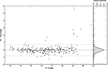
Figure 2: Difference between the R1 and R2 magnitudes as a function of the R1 magnitude for the USNO-B matches of the combined sample. The density estimate is also represented (grey). It is roughly normal (dashed curve), centered around -0.04 mag and with a width of $\sigma$=0.26 mag. Any USNO-B source outside the $\pm$3-$\sigma$ limits was discarded.

5 Membership

Figure 3 shows the vector point diagrams obtained with USNO-B and UCAC2 proper motion measurements for the combined sample. A clustering appears clearly around ($\mu_{\alpha}\cos{\delta},\mu_{\delta}$) = (-6.7,-19.3) mas yr^-1 (USNO-B) and ($\mu_{\alpha}\cos{\delta},\mu_{\delta}$) = (-9.1,-24.7) mas yr^-1 (UCAC2) and we associate it with the Upper Scorpius co-moving group. A significant number of objects fall far away from the co-moving group.

Proper motion can be used to quantitatively assess the membership of objects in a co-moving group. As described in Sanders (1971), the distribution of proper motion in a vector point diagram can be modeled by two independent overlapping distributions of member and interloper stars. In this model, the proper motion dispersion of members is assumed to be caused by observational and measurement errors normally distributed, so that the distribution of member stars is represented by a bivariate normal distribution. Unlike in the cases described by Sanders (1971), all the objects of our sample have been selected based on their spectroscopic characteristics, so that the contribution of non-members to the vector point diagram is mainly due to coincident young sources. We consider that their distribution in the vector point diagram is constant over the parameter space probed by our analysis and model it with a uniform function. A 2-D Gaussian + constant function is thus fitted to the 2-D kernel density estimate of the vector point diagram and we obtain:

$$f_{m\,\rm USNO}(\mu_{\alpha}\cos{\delta},\mu_{\delta}) = 0.0061\exp\Bigg{\{}-\frac{1}{2}\Biggl{[}\Bigg{(}\frac{\mu_{\alpha}\cos{\delta}+6.7}{5.0}\Bigg{)}^{2}$$

$$+ \Bigg{(}\frac{\mu_{\delta}+19.3}{5.2}\Bigg{)}^{2}\Biggl{]}\Bigg{\}}$$

$$f_{m\,\rm UCAC2}(\mu_{\alpha}\cos{\delta},\mu_{\delta}) = 0.0022\exp\Bigg{\{}-\frac{1}{2}\Biggl{[}\Bigg{(}\frac{\mu_{\alpha}\cos{\delta}+9.1}{8.7}\Bigg{)}^{2}$$

$$+ \Bigg{(}\frac{\mu_{\delta}+24.7}{8.1}\Bigg{)}^{2}\Biggl{]}\Bigg{\}}$$

and

$$f_{i\,\rm USNO}(\mu_{\alpha}\cos{\delta},\mu_{\delta})=2.9\times 10^{-6}$$

$$f_{i\,\rm UCAC2}(\mu_{\alpha}\cos{\delta},\mu_{\delta})=1.5\times 10^{-6}$$

where $f_{m}(\mu_{\alpha}\cos{\delta},\mu_{\delta})$ and $f_{i}(\mu_{\alpha}\cos{\delta},\mu_{\delta})$ are the vector point distributions of respectively the members and interlopers. The membership probability can then be computed as:

$$\mathcal{P}=\frac{f_{m}(\mu_{\alpha}\cos{\delta},\mu_{\delta})}{f_{m}(\mu_{\alpha}\cos{\delta},\mu_{\delta})+f_{i}(\mu_{\alpha}\cos{\delta},\mu_{\delta})}$$

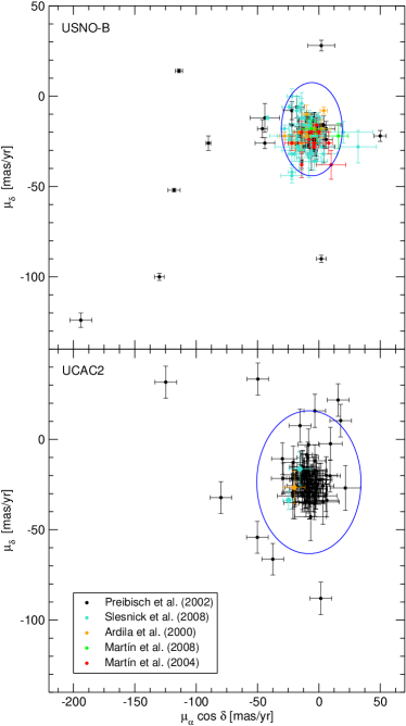
Figure 3: Vector point diagrams for the spectroscopically confirmed members of Upper Scorpius with USNO-B (upper panel) and UCAC2 (lower panel) counterparts. Blue ellipses represent the $\mathcal{P}=$0.1% membership probability level used to select outliers candidates.

For the rest of the discussion we classify as highly probable members objects that are located inside the $\mathcal{P}=$0.1% (3-$\sigma$) membership probability ellipse within the uncertainties, and as candidate outliers objects outside the $\mathcal{P}=$0.1% membership probability ellipse. Even though this arbitrary threshold probably misses a number of outliers, it offers the advantage of separating obvious outliers from the overall co-moving group. The main goal for the rest of this paper is to confirm, identify and characterize the properties of these obvious outliers. The task of drawing firmer statistical conclusions regarding their frequency is left to more detailed studies of complete samples using higher proper motion accuracy. A total of 16 outliers are found in the USNO-B analysis and 9 in the UCAC2 analysis. We note that 3 objects (UScoCTIO-101, SCHJ16162599-21122315 and SCHJ16211564-24361173) have a probability membership less than 30%. We classify them as likely outliers, but do not include them in the rest of our analysis for consistency.

6 Reality of the outliers

Because of the sample size, a human inspection of each USNO-B and UCAC2 counterpart is not possible. The rejection of doubtful objects described in section 4 is purely statistical. Problematic sources might remain in the final sample. Outliers are of course suspicious in nature and deserve a more careful inspection before any further discussion can be made.

6.1 Overlap between USNO-B and UCAC2

A total of 66 objects of the combined sample have a counterpart in both the USNO-B and UCAC2 catalogues (see Table 6). As mentioned above, the systematic errors of each catalogues prevent us from making a direct comparison between the USNO-B and UCAC2 proper motion measurements. On the other hand, the consistency of the membership probability for the 66 sources in common provides an important check of the reliability of the two analyses. Table 6 shows that the membership probabilities derived independently using USNO-B and UCAC2 indeed agree well within $\pm$2% for all 66 objects in common except for one (USco-161437.52-185824.0). With a membership probability of 80% in USNO-B, and 99.2% in UCAC2, we nevertheless classify this latter source as a highly probable member. Moreover, four of the 16 outliers found in the USNO-B analysis have a UCAC2 counterpart. All four are independently classified as outliers by the UCAC2 analysis as well. The two surveys being based on completely independent datasets, this comparison demonstrates the reliability and robustness of our membership analysis and classification criterion.

6.2 Probability estimator (USNO-B)

Proper motions in the USNO-B catalogue are given with their uncertainties as well as a probability estimator for the likelihood that the proper motion is correct. This estimator ranges between 0.1 and 0.9, a larger value corresponding to a higher probability of being correct. It is a measurement of the goodness of fit between the observed motion over N_obs epochs reported in the catalogue and the linear motion fit. It is computed from the integral probability that the sample of N_obs random observations would yield an experimental linear-correlation as large or larger than the observed one (as described in Bevington & Robinson, 1992, D. Monet, private communication).

For equal values of the probability estimator, sources with N_obs=3 have a less believable proper motion measurements than sources with N${}_{\rm obs}\geq$4. The probability estimator is therefore not enough in itself to assess the reliability of the proper motion measurements. We note that at least 3 epochs have been used for all the USNO-B counterparts in our analysis. In fact, 69% of the sources in our study have been reported 5 times out of 5 epochs, and 26% of them have been reported 4 times out of 5 epochs (see Table 6) while only 5% have been reported 3 times only out of 5 epochs. Only 1 out of the 16 outliers identified in the USNO-B survey has been reported 3 times only out of 5 epochs (SCHJ16162599-21122315). The probability estimator are therefore believed to be reliable for the 15 others. All 15 have a probability estimator of 0.9 estimated over 4 epochs or more (see Table 6).

6.3 Visual inspection

False detections as well as multiple systems are the main source of error for the USNO-B proper motion measurements (D. Monet, private communication). The USNO-B Schmidt plate 5 epoch images are available on-line. We retrieved the data for all 16 outliers identified in the USNO-B analysis as well as the corresponding 2MASS (Skrutskie et al., 2006), DENIS (Fouqué et al., 2000) and UKIDSS (Lawrence et al., 2007) images of both USNO-B and UCAC2 outliers when available to check the quality of the multi-epoch detections and the eventual presence of blended companions. Two objects are resolved as multiple systems and are discarded for the rest of the analysis.

USco-160726.8-185521 is resolved as a binary in Bouy et al. (2006) adaptive optics images with a separation of 3$\aas@@fstack{\prime\prime}$191, a position angle of 353.1°  and a difference of magnitude in Ks of $\Delta m$=2.0 mag. It is also clearly elongated in the 2MASS images. The UCAC2 proper motion measurement is therefore suspicious and this object is removed from the list of outlier candidates.

SCH J16202523-23160347 is elongated or resolved as a close blended visual binary in most USNO-B images. It is also elongated in the 2MASS images and detected but unresolved in the DENIS images. The source is clearly resolved in the UKIDSS images as a visual triple system. This interesting object is discussed in more detail in Appendix A, and is removed from the list of outlier candidates for the rest of the discussion as the presence of visual companions might have affected the USNO-B proper motion measurement.

A total of 19 outliers (15 identified in USNO-B and 4 in UCAC2) remain after the visual inspection.

7 Kinematic properties of the Upper Scorpius population

Figure 4 shows the distribution of transverse velocities as a function of spectral type. No significant dependence on the spectral type can be seen for co-moving members within the relatively large individual uncertainties and overall dispersion. These uncertainties ($\approx$6 mas yr^-1 in average for USNO-B, corresponding to $\approx$4 km s^-1 at the distance of Upper Scorpius) are larger than the difference in dispersion velocities between stars and VLM objects expected from dynamical interactions in the early stages of young proto-stellar clusters ($\approx$2 km s^-1, Kroupa & Bouvier, 2003; Sterzik & Durisen, 2003; Bate, 2009). More accurate measurements are therefore required to improve this upper limit and make a detailed comparison of the kinematics of stellar and substellar members. Finally, we note that the spectral type distributions among outliers and members are indistinguishable at the 83% confidence level as established by a Kolmogorov-Smirnov test.

Figure 4: Transverse velocities as a function of spectral type for the USNO-B (left) and UCAC2 (right) analysis. Co-moving members are represented with grey dots, and outliers with red dots. The mean velocities (solid line) and the $\pm$3-$\sigma$ dispersion (dashed lines) of the association computed in section 5 are also represented. There is no difference between early and late spectral types members within the individual uncertainties and overall dispersion.

8 Nature of the contaminants

All the objects in the initial sample were confirmed as members of the association based on spectroscopic characteristics unambiguously associated with youth (atomic and/or molecular age diagnostics such as the presence and strength of Li and Na I absorption, or H$\alpha$ emission). These different diagnostics correspond to different limits on the age of these objects. Preibisch et al. (2002) Li selection criterion places an upper limit on the age at $\lesssim$30 Myr. Slesnick et al. (2008) Na I criterion (which is similar to that of Martín et al., 2004, 2009) is less restrictive and places an upper limit at about $\lesssim$100 Myr. The H$\alpha$ criterion of Ardila et al. (2000) was defined to select candidate in the range $\approx$5–50 Myr. The 21 outliers are therefore young ($\lesssim$100 Myr) free floating objects that could either have been ejected from neighboring associations, belong to unknown coincident foreground associations, or have recently experienced dynamical interactions within the Upper Scorpius association. Figure 5 shows a map of the Upper Scorpius region with the sample over-plotted.

Figure 5: Spatial distribution of LMSs, VLMSs and BDs in our sample over-plotted on an IRAS 12 $\mu$m image for the USNO-B analysis (left) and UCAC2 analysis (right). Spectroscopically confirmed members with proper motion consistent with the co-moving group are represented by black dots. Candidate outliers are represented with red dots. Hipparcos members from de Zeeuw et al. (1999) are represented with blue stars with sizes proportional to their V-band luminosities. The segments represent the objects motions over the past 100 000 yr, assuming constant proper motions and null radial velocities. The densest nebulosity in the lower left quadrant are part of the $\rho-$Oph molecular cloud.

8.1 Accretor frequency among outliers and members

Low resolution optical spectra have been obtained for all the objects, and measurements of H$\alpha$ equivalent width have been published. Our outlier selection criterion based on the proper motion membership probability is completely independent from the H$\alpha$ equivalent width, and hence we can use H$\alpha$ to make an unbiased comparison between the accretor frequency among kinematic outliers and members in the co-moving group. Figure 6 shows the H$\alpha$ equivalent width as a function of spectral type, and the chromospheric criterion defined by Barrado y Navascués & Martín (2003) to distinguish between chromospheric activity and accretion induced H$\alpha$ emission. According to this criterion, a total of 25 of the 229 co-moving members found in the combined USNO-B and UCAC2 samples are accretors, while none of the 19 outlier candidates is accreting. The accretor frequency for members (11%) is higher than the upper limit observed for outliers ($<$5%), but only at the 77% confidence level, as determined from the two-tailed Fisher’s Exact Test (Fisher, 1922). The difference between the outliers and members accretor frequencies is not statistically conclusive.

Figure 6: H$\alpha$ equivalent width (in Å) versus spectral type. Co-moving objects are represented with grey diamonds, and candidate outlier with red dots. Upper limits are represented with triangles and the same color code. The chromospheric criterion of Barrado y Navascués & Martín (2003) is represented with a dashed line. According to this criterion, none of the outliers is accreting.

8.2 Disk frequency among outliers: mid-infrared observations

We searched the Spitzer Space Telescope public archive for images of the sample of 19 outliers. We found that 9 of them fall in the field of view of IRAC and/or MIPS observations as part of programs 148 (P.I. Meyer), 177 (P.I. Evans), 20069 (P.I. Carpenter) and 58 (P.I. Rieke). We retrieved the pipeline processed data and extracted PSF photometry of the outliers when detected, and flux upper limits when undetected. The photometry was extracted using standard PSF photometry procedures within the Interactive Data Language. Uncertainties were estimated from the Poisson noise weighted by the coverage maps of the mosaics, but are in general dominated by the flux calibration uncertainties. Upper limits were estimated by adding artificial stars of decreasing luminosity until the 3-$\sigma$ detection algorithm misses it. The results are given in Table 3 and Fig. 7. The mid-infrared (mid-IR) observations allow us to put constraints on the presence of hot circumstellar inner disks around these outliers. The single flux upper limit at 24 $\mu$m available for USco-160028.5 does not allow us to conclude on the presence of mid-IR excess. None of the other nine outliers display mid-IR excess. Recent studies based on similar analyses found a mid-IR excess fraction of 22% among Upper Scorpius K0–M9 members (37 out of 162 members for the combined surveys of Carpenter et al., 2006; Scholz et al., 2007), larger than that for outliers (0 out of 9) but at the 63% confidence level only (as determined from the two-tailed Fisher’s Exact Test). The difference is therefore statistically inconclusive.

8.3 Photometric distances

We use the spectral energy distribution (SED) to estimate the photometric distances to the outliers. The SED are unreddened using the extinction measurements provided by the different discoverers, or assuming an average A_V=1.4 mag as reported in Preibisch et al. (2002) when no measurement is available. The spectral types are translated into effective temperatures using the temperature scale given in Luhman et al. (2003). Considering the age limit given in section 8, we derive the photometric distance by fitting the unreddened SED with the corresponding NextGen photospheric SED (Baraffe et al., 1998) for ages of 5, 50 and 100 Myr. In each case the best fit is obtained using a $\chi^{2}$ minimization with the distance being the only free parameter. The results are displayed in Table 4. Using Hipparcos, de Zeeuw et al. (1999) estimated an average distance to the association of 145 pc, while Martín (1998) suggested the presence of some LMS members as close as 80 pc from the Sun. In order to be conservative, we hereafter consider that any object within 145$\pm$65 pc is in the distance range of the association. If 5 Myr old, the outliers must be located approximately within 99–443 pc and 11 of them have photometric distances consistent with the association. The remaining eight all have distances greater than that of the association, and are therefore most likely background coindicences. If 100 Myr old, the outliers must be located approximately within 33–131, and 8 of them have photometric distances consistent with the boundaries of the association.

Table 3: Spitzer IRAC and MIPS photometry of the outliers

Objects	3.6 $\mu$m	4.5 $\mu$m	5.8 $\mu$m	8.0 $\mu$m	24 $\mu$m
	[mJy]	[mJy]	[mJy]	[mJy]	[mJy]
SCHJ16324224					0.74$\pm$0.14
Usco-155744.9	18.6$\pm$1.9		8.9$\pm$0.9
USco-160028.5					$<$0.9
USco-160325.6					$<$0.3
USco-160407.7	4.1$\pm$0.4		2.3$\pm$0.2
USco-160745.8	2.9$\pm$0.3		1.3$\pm$0.2
USco-160926.7					0.3$\pm$0.03
USco-161021.5		30.0$\pm$0.3		12.3$\pm$0.1	0.5$\pm$0.05
SCHJ162215.8	3.3$\pm$0.3	2.2$\pm$0.2	1.6$\pm$0.2	0.9$\pm$0.1

Table 4: Photometric distances to the outliers assuming various ages

Objects	SpT	d (5 Myr)	d (100 Myr)
		[pc]	[pc]
SCHJ15582566-18260865	M6	115	44
SCHJ16084058-22255726	M4	439	130
SCHJ16221577-23134936	M6	176	68
SCHJ16324224-23165644	M5.5	99	33
USco-155744.89-222351.1	M2	294	85
USco-155848.44-224658.4	M0	443	131
USco-155930.21-225126.2	M4	293	87
USco-160017.34-221811.1	M6	148	57
USco-160028.47-220922.6	M6	170	66
USco-160054.45-224908.9	M3	195	62
USco-160142.6-222923	M0	270	81
USco-160236.21-191732.5	M3	346	109
USco-160325.6-194438	M2	379	108
USco-160407.73-194857.9	M5	186	69
USco-160522.69-205112.1	M4	159	47
USco-160745.74-203055.7	M3	422	134
USco-160845.6-182443	M3	150	48
USco-160926.71-192502.5	M3	210	67
USco-161021.5-194132	M3	107	34

Figure 7: Spectral energy distributions of the 9 outliers with available Spitzer photometry (black dots). The NextGen theoretical spectra of the corresponding effective temperature are over-plotted as dashed lines. The single flux upper limit at 24 $\mu$m available for USco-160028.5 does not allow to conclude on the presence of mid-IR excess. None of the other nine outliers display mid-IR excess.

9 Origin of the outliers

Proper motions only are not enough to trace back the origin of objects, as the age, distance and radial velocities would be required to fully understand where they come from. Over long timescales (typically greater than $\approx$10 000 yr), the radial motion will cause a significant change in the distance and therefore in the apparent transverse velocity. Associations might also be rotating, adding another unknown to the equation. With these limitations in mind, we try to discuss the origin of the outlier candidates identified in our analysis.

9.1 Ejected members of Upper Scorpius

Using the current proper motions we can tentatively trace back the location of the outliers and check whether they could originate from the Upper Scorpius association. Outliers identified in our study have proper motion amplitudes in the range 25$\sim$230 mas yr^-1. For them to remain in the field of the discovery surveys ($\approx$15°$\times$15°at most, see Fig 5), the interactions should have occurred less than 0.25–2.2 Myr ago (assuming a null radial velocity and constant proper motion). The probability for dynamical interactions to occur decreases rapidly with time after the first few 0.1 Myr of the formation of the parent proto-stellar cores (Bate, 2009). Dynamical interactions within the loose Upper Scorpius association are therefore extremely unlikely within the past 2.2 Myr. These simple statistical considerations suggest that the fastest outlier candidates are most likely not ejected members of the Upper Scorpius association itself.

9.2 Upper Scorpius A and B

Even though the original surveys used in our study were all performed in Upper Scorpius A, some spatial overlap with Upper Scorpius B (USco B) cannot be ruled out. Some of the outliers candidates identified in our study could be either coincident USco B members or ejected USco B members. Kraus & Hillenbrand (2007a) assigned a mean proper motion of (-10,-25) mas yr^-1 for USco A and (-21.3,-25.5) mas yr^-1 for USco B. The difference between the two subgroups mean proper motions is of the same order or smaller than the uncertainties on the USNO-B and UCAC2 measurements, so that an USco B members would most likely fall within the selection criterion defined in section 5. While the age and distance of USco A are well constrained thanks to the presence of high-mass members with Hipparcos measurements, the properties and history of USco B are poorly known, making it difficult to test whether some of the outliers could be USco B members.

9.3 Neighboring associations

Upper Scorpius is part of the Sco-Cen complex (de Geus et al., 1989) and is surrounded by the Upper Centaurus Lupus (13 Myr at 160 pc) and Lower Centaurus Crux (10 Myr at 118 pc) associations. Comparing the outliers proper motions to the mean proper motion of these loose associations would be meaningless given the distances between these associations and the corresponding large projection effects. Improved proper motion measurements as well as distance and radial velocity measurements will be required to perform a detailed comparison in the $(U,V,W)$ plane.

The 1 Myr old $\rho-$Oph association is located on the south-eastern part of Upper Scorpius (see Fig. 5) and is sufficiently close that projection effects on the proper motions are smaller than the typical uncertainties of the USNO-B and UCAC2 measurements. Mamajek (2008) recently estimated its distance to be 139$\pm$6 pc. Assuming that they are young, a number of outliers have photometric distances in the range 100–170 pc and could possibly originate from $\rho-$Oph.

9.4 Nearby coincident associations

Even within their large uncertainties, the photometric distances indicate that a number of outliers are nearby and cannot belong to the more distant Upper Scorpius association. These objects could be members of coincident young nearby associations such as AB Dor or $\beta-$Pic (Torres et al., 2008). Membership of these associations can only be inferred in the $(U,V,W)$ plane and therefore requires accurate radial velocity and distance measurements.

10 Discussion

Our study shows that 19 objects out of the combined sample of 251 objects (USNO-B+UCAC2) selected photometrically and confirmed spectroscopically have proper motion inconsistent with that of the Upper Scorpius association. If these outliers have the same age as the Upper Scorpius assocition, then 11 of them have photometric distances consistent with that of the association and could be genuine members having recently experienced dynamical interactions. Although this latter hypothesis cannot be rules out, the low probability for such interactions to have occured within the loose Upper Scorpius association nevertheless suggests that most of these outliers are background or foreground coincidences. Such contaminants are a well known problem that plagues the study of the initial mass function low mass end based on photometric surveys only. Kirkpatrick et al. (2008) and Valdivielso et al. (2009) have recently reported a number of young free floating very low mass objects in the field, suggesting that the contamination of photometrically selected samples of young associations could remain significant even after spectroscopic confirmation.

With 19 outliers among a total sample of 251 objects, we derive an observed outlier frequency of 7.6$\pm$1.8%. The current statistics has several limitations and this value should be considered with caution. As previously mentioned, our membership criterion was not meant to derive a statistically complete sample of outliers. Instead it was defined conservatively to separate the most obvious outliers from the association members. It therefore probably misses a number of contaminants. Moreover limiting the search radius to 3″  additionally introduces a bias toward smaller proper motions, but increasing it also considerably increases the number of erroneous sources as objects with greater proper motions have a higher probability of being spurious entries in the catalogues. UCAC2 sources with proper motion greater than 0$\aas@@fstack{\prime\prime}$2 yr^-1 were systematically rejected from the catalogue. The outlier frequency derived from the current analysis should be regarded as a preliminary lower limit.

11 Conclusions and future prospects

We have cross-matched catalogues of low, very low mass and substellar objects classified as members of the Upper Scorpius association based on their photometric and spectroscopic characteristics with the USNO-B and UCAC2 catalogues. Our conclusions are threefold:

• a significant fraction of them have proper motion measurements reported in the USNO-B and UCAC2 catalogues. We find an observed frequency of 7.6$\pm$1.8 (19 out of 251) of objects with proper motions inconsistent with that of the co-moving group. This value is only a preliminary lower limit since our analysis suffers from a number of biases and incompleteness. Improved studies based on statistically complete samples and using more accurate proper motion measurements are required to derive accurate values of the outlier frequency.

• The outliers must be either free-floating young objects wandering after being ejected from a neighboring association, members of coincident foreground associations, or members of the association having experienced dynamical interactions within the past 0.2–2.2 Myr. The observed accretor and disc frequencies are lower among outliers than among members, but the current small-number statistics does not allow us to draw firm conclusions.

• to minimize this source of contamination, comprehensive surveys should be based on photometrically, spectroscopically and kinematically confirmed members.

Follow-up observations of the non-members are required to understand their origin. In particular, the study of their multiplicity and how it compares to Upper Scorpius members could provide hints on whether these objects went through ejection events. Only short separation multiple systems are expected to survive the dynamical interactions responsible for the ejection. These processes are also expected to imprint a distinct secondary mass function on multiple systems. Finally, radial velocity and parallax measurements could help trace back their origin and whether they simply belong to unknown foreground associations or were ejected from the association or from a neighboring association. In the latter cases, kinematics offers a unique opportunity to identify ejected young low and very low mass objects. Understanding their origin and history holds important clues on the contribution of ejection phenomenons to the formation of low and very low mass objects. Kinematics will thus certainly play a key role to identify objects having experienced dynamical interactions, to quantify the contribution of ejection to the formation of very low mass objects, and understand the consequences of dynamical ejection on the formation and evolution of very low mass objects.

Appendix A SCH J16202523-23160347

Figure 8 shows that SCH J16202523-23160347 is either resolved or elongated in most USNO-B images as well as in the 2MASS images. It is clearly resolved as a visual triple system in the H and K-band UKIDSS images. Unfortunetaly, the current UKIDSS data release does not include Z, Y or J band images of this field. Whereas at optical wavelengths the southern component is more luminous, the northern component is significantly brighter from 1.6 $\mu$m to longer wavelengths. We call the brightest optical component in the following the primary. The UKIDSS catalogue reports detection of only the primary (blended with the tertiary) and the secondary. In order to measure the astrometry and photometry of all three components, we retrieved the H and K band images from the UKIDSS server and extracted the photometry using PSF photometry with the Starfinder code (Diolaiti et al. 2000). The zeropoints were computed using the UKIDSS photometry of component B. The results are given in Table 5

The quality of the USNO-B images does not allow to measure useful relative astrometry of the components to check common proper motion. Assuming that the system is member of Upper Scorpius and shares the mean proper motion of the association, a background source would have moved by $\approx$0$\aas@@fstack{\prime\prime}$6 between these 2 epochs. Such a motion is unfortunately smaller than the relative astrometric accuracy achievable in the USNO-B images.

The unresolved system was classified as M5.5 by Slesnick et al. (2008), but their spectrum might have been affected by the dominating contribution of the blue primary. The H and K band photometry corresponds to a spectral type of $\approx$M8. SCH J16202523-23160347A is therefore very likely a brown dwarf. Figure 9 shows a color-magnitude diagram of known members from the literature with the three components over-plotted. While B has colors and luminosities consistent with those of very low mass members of the association, A and C lie far off the tracks. They are therefore most likely not members of the association but coincident sources.

Figure 8: AAO-R (1991.23) and UKIDSS-Ks (2005.46) images of SCH J16202523-23160347. The source is clearly elongated in the AAO image, and resolved as a triple system in the UKIDSS image. North is up and east is left, and the scale is indicated.

Figure 9: H vs H-K color-magnitude diagram for SCH J16202523-23160347 and compared to Upper Scorpius very low mass members from the literature including 2 very low mass multiple systems (Béjar et al. 2008; Kraus & Hillenbrand 2007c). The B component has luminosities and colors consistent with those of very low mass members. The A et B components luminosities and colors are inconsistent with those of very low mass members. The DUSTY (Baraffe et al. 2002) and COND (Baraffe et al. 2003) isochrones at the distance of Upper Sco are over-plotted.

Table 5: Photometric and astrometric properties of the visual triple system SCH J16202523-23160347

Component	H	K	Sep.	P.A
B	13.711$\pm$0.002	13.213$\pm$0.003	2$\aas@@fstack{\prime\prime}$618$\pm$0.003	8.68°$\pm$0.09°
A	16.33$\pm$0.02	16.12$\pm$0.03
C	18.05$\pm$0.09	17.39$\pm$0.09	0$\aas@@fstack{\prime\prime}$915$\pm$0.015	245°$\pm$4°

3

Table 6: Sample of Upper Scorpius objects with a counterpart in the USNO-B only or USNO-B and UCAC2 catalogues

Literature							USNO-B										UCAC2
Name	R.A	Dec.	SpT	R	I	$W(\rm H\alpha)$	$r$	Mean	Nobs	R1	R2	I	$\mu_{\alpha}\cos\delta$	$\mu_{\delta}$	$\mu_{\rm Prob}$	Prob.	$r$	$\mu_{\alpha}\cos\delta$	$\mu_{\delta}$	Prob.
	(J2000)	(J2000)		[mag]	[mag]	[Å]	[″]	Epoch		[mag]	[mag]	[mag]	[mas yr-1]	[mas yr-1]	[0.1]	[%]	[″]	[mas yr-1]	[mas yr-1]	[%]
Preibisch et al. (2002)
USco-155625.64-224027.0	15 56 25.6	-22 40 27.0	M3	14.6		-4.2	0.812	1972.3	5	14.85	14.64	13.17	-8$\pm$3	-18$\pm$4	9	99.9	0.236	-9.9$\pm$8.9	-18.9$\pm$8.9	99.9
USco-155629.51-225657.7	15 56 29.5	-22 56 57.7	M3	14.3		-3.1	0.680	1972.3	5	14.52	14.35	13.03	-4$\pm$4	-12$\pm$3	9	99.9
USco-155706.41-220605.7	15 57 06.4	-22 06 05.7	M4	16.2		-3.6	0.298	1972.3	5	16.44	16.25	14.30	-18$\pm$6	-6$\pm$6	9	85.9
USco-155728.49-221905.1	15 57 28.4	-22 19 05.1	M5	16.7		-6.2	1.085	1972.3	5	16.78	16.83	14.64	-8$\pm$9	-26$\pm$4	9	99.9
USco-155729.87-225843.7	15 57 29.8	-22 58 43.7	M4	15.8		-7.0	0.832	1972.3	5	15.95	15.80	14.02	-6$\pm$0	-16$\pm$7	8	99.9
USco-155742.50-222605.3	15 57 42.5	-22 26 05.3	M3	15.7		-2.9	0.263	1972.3	5	15.98	15.73	14.01	-18$\pm$10	-22$\pm$5	9	99.3
USco-155744.89-222351.1	15 57 44.8	-22 23 51.1	M2	14.3		-0.9	0.178	1972.3	5	14.75	14.11	13.29	2$\pm$11	28$\pm$3	9	$\ll$0.1	0.617	17.8$\pm$8.8	10.4$\pm$9.0	0.1
USco-155746.63-222920.1	15 57 46.6	-22 29 20.1	M3	14.7		-2.1	1.147	1972.3	5	15.19	14.73	13.33	-8$\pm$3	-18$\pm$5	9	99.9	0.240	-9.4$\pm$8.8	-18.1$\pm$9.5	99.9
USco-155829.83-231007.4	15 58 29.8	-23 10 07.4	M3	15.4		-250.0	0.578	1972.3	5	14.72	14.61	14.19	-8$\pm$5	-18$\pm$3	9	99.9
USco-155848.44-224658.4	15 58 48.4	-22 46 58.4	M0	14.5		-0.5	2.645	1972.3	5	14.74	14.31	13.53	-194$\pm$9	-124$\pm$4	9	$\ll$0.1
USco-155912.51-223650.3	15 59 12.5	-22 36 50.3	M5	16.4		-10.5	0.280	1972.3	5	16.93	16.54	14.60	4$\pm$9	-28$\pm$9	8	98.1
USco-155918.38-221043.0	15 59 18.3	-22 10 43.0	M4	14.7		-1.0	1.010	1972.3	5	14.91	14.92	13.16	-14$\pm$4	-24$\pm$1	9	99.8	0.213	-0.6$\pm$9.1	-24.8$\pm$9.3	99.9
USco-155925.92-230508.1	15 59 25.9	-23 05 08.1	M6	17.0		-19.5	0.247	1972.3	5	17.22	17.24	14.73	-14$\pm$9	-26$\pm$5	9	99.7
USco-155930.21-225126.2	15 59 30.2	-22 51 26.2	M4	17.6		-5.0	1.917	1976.8	4	17.61	17.55	15.41	50$\pm$5	-22$\pm$3	9	$\ll$0.1
USco-160007.14-222406.6	16 00 07.1	-22 24 06.6	M4	16.8		-4.4	1.038	1972.3	5	16.54	16.79	15.01	-22$\pm$7	-8$\pm$5	9	65.1
USco-160017.34-221811.1	16 00 17.3	-22 18 11.1	M6	16.5		-3.9	1.415	1972.3	5	16.97	16.56	14.59	-130$\pm$4	-100$\pm$2	9	$\ll$0.1
USco-160018.46-223011.6	16 00 18.4	-22 30 11.6	M3	14.7		-150.0	1.009	1972.3	5	14.65	15.18	13.53	-2$\pm$5	-26$\pm$9	8	99.8	0.453	-10.4$\pm$4.6	-20.3$\pm$4.6	99.9
USco-160028.47-220922.6	16 00 28.4	-22 09 22.6	M6	16.8		$>$-0.04	0.734	1972.3	5	17.39	16.82	14.91	-44$\pm$12	-12$\pm$8	9	$\ll$0.1
USco-160030.24-233445.3	16 00 30.2	-23 34 45.3	M6	17.2		-15.8	0.663	1974.0	5	17.77	17.46	14.98	-16$\pm$5	-20$\pm$1	9	99.7
USco-160054.45-224908.9	16 00 54.4	-22 49 08.9	M3	14.7		$>$-0.04	1.138	1972.3	5	14.98	15.05	13.36	-118$\pm$5	-52$\pm$1	9	$\ll$0.1	0.143	-79.8$\pm$8.8	-32.2$\pm$8.8	$\ll$0.1
USco-160110.37-222227.7	16 01 10.3	-22 22 27.7	M4	14.2		-9.4	0.885	1972.3	5	14.78	14.63	12.80	-12$\pm$4	-28$\pm$3	9	99.7	0.098	-3.2$\pm$8.8	-33.7$\pm$8.9	99.8
USco-160121.56-223726.5	16 01 21.5	-22 37 26.5	M4	14.2		-8.4	1.009	1972.3	5	14.66	14.63	12.73	-10$\pm$3	-18$\pm$4	9	99.9	0.049	-11.1$\pm$9.7	-29.1$\pm$9.0	99.9
USco-160129.85-224838.6	16 01 29.8	-22 48 38.6	M4	14.9		-4.4	0.863	1972.3	5	15.51	15.57	13.26	-10$\pm$3	-28$\pm$1	9	99.8	0.183	-19.9$\pm$9.0	-28.9$\pm$8.6	99.8
USco-160140.87-225810.5	16 01 40.8	-22 58 10.5	M3	14.0		-120.0	1.119	1972.3	5	14.55	13.99	13.06	-8$\pm$1	-28$\pm$4	9	99.8	0.018	-18.9$\pm$8.7	-26.7$\pm$9.8	99.9
USco-160158.96-224036.6	16 01 58.9	-22 40 36.6	M4	14.4		-7.6	1.004	1972.3	5	15.10	14.81	13.09	-14$\pm$3	-20$\pm$0	9	99.9	0.413	-19.6$\pm$8.8	-35.1$\pm$8.8	99.7
USco-160202.90-223613.9	16 02 02.9	-22 36 13.9	M0	14.7		-1.5	0.883	1972.3	5	14.95	14.88	13.50	-8$\pm$5	-26$\pm$3	9	99.9	0.770	-29.1$\pm$9.6	-21.6$\pm$8.6	99.0
USco-160207.57-225746.7	16 02 07.5	-22 57 46.7	M1	13.7		-3.2	1.249	1972.3	5	14.36	13.69	12.66	-16$\pm$1	-20$\pm$6	9	99.7	0.203	-13.5$\pm$8.7	-20.0$\pm$8.8	99.9
USco-160210.95-200749.7	16 02 10.9	-20 07 49.7	M5	16.4		-3.5	0.961	1970.8	5	16.55	16.54	14.35	-6$\pm$5	-22$\pm$5	9	99.9
USco-160222.43-195653.8	16 02 22.4	-19 56 53.8	M3	14.7		-6.6	0.897	1970.8	5	14.72	14.63	13.14	-22$\pm$2	-16$\pm$9	9	94.4
USco-160236.21-191732.5	16 02 36.2	-19 17 32.5	M3	17.3		-0.7	0.531	1970.8	5	16.71	17.00	15.31	-44$\pm$8	-26$\pm$3	9	$\ll$0.1
USco-160245.45-193038.1	16 02 45.4	-19 30 38.1	M5	16.4		-1.1	1.327	1970.8	5	16.16	16.69	14.28	-4$\pm$1	-24$\pm$1	9	99.9
USco-160245.75-230450.6	16 02 45.7	-23 04 50.6	M6	16.7		-100.0	0.935	1972.3	5	16.92	16.91	14.55	-20$\pm$4	-26$\pm$4	9	96.5
USco-160258.56-225649.5	16 02 58.5	-22 56 49.5	M2	13.9		-9.4	0.962	1972.3	5	14.21	14.02	12.74	-4$\pm$3	-24$\pm$3	9	99.9	0.087	-7.4$\pm$4.5	-19.9$\pm$4.5	99.9
USco-160329.40-195503.8	16 03 29.4	-19 55 03.8	M5	15.7		-4.9	0.754	1970.8	5	15.85	15.93	13.97	-8$\pm$2	-14$\pm$6	8	99.9
USco-160341.87-200557.8	16 03 41.8	-20 05 57.8	M2	13.5		-2.2	1.318	1970.8	5	13.79	13.56	12.45	-8$\pm$1	-22$\pm$5	9	99.9	0.101	-8.4$\pm$8.7	-29.7$\pm$8.7	99.9
USco-160343.34-201531.6	16 03 43.3	-20 15 31.6	M2	13.6		-3.5	0.778	1970.8	5	13.69	13.68	12.58	-12$\pm$2	-18$\pm$2	9	99.9	0.149	-10.3$\pm$8.7	-29.2$\pm$8.6	99.9
USco-160350.47-194121.6	16 03 50.4	-19 41 21.6	M5	15.0		-4.9	1.180	1970.8	5	14.90	15.23	13.41	-2$\pm$1	-12$\pm$2	9	99.8	0.034	-8.4$\pm$8.7	-31.9$\pm$8.8	99.9
USco-160357.93-194211.0	16 03 57.9	-19 42 11.0	M2	14.5		-3.0	1.076	1970.8	5	14.67	14.63	13.14	-8$\pm$6	-20$\pm$2	9	99.9	0.098	-10.2$\pm$8.7	-25.2$\pm$8.7	99.9
USco-160407.73-194857.9	16 04 07.7	-19 48 57.9	M5	16.8		-4.0	1.041	1970.8	5	16.77	16.73	14.74	-46$\pm$4	-18$\pm$5	9	$\ll$0.1
USco-160418.20-191055.7	16 04 18.2	-19 10 55.7	M4	15.4		-0.5	0.736	1970.8	5	15.65	15.72	13.69	-8$\pm$4	-12$\pm$2	9	99.9	0.270	9.1$\pm$8.5	-20.2$\pm$8.9	99.3
USco-160435.64-194830.3	16 04 35.6	-19 48 30.3	M5	16.1		-7.2	0.670	1970.8	5	16.32	17.11	14.68	-10$\pm$4	-20$\pm$2	9	99.9
USco-160439.17-194245.9	16 04 39.1	-19 42 45.9	M4	15.1		-3.8	1.285	1970.8	5	15.18	15.45	13.46	-8$\pm$3	-12$\pm$2	9	99.9	0.041	-9.0$\pm$8.8	-10.1$\pm$8.6	99.7
USco-160449.96-203835.5	16 04 49.9	-20 38 35.5	M5	16.0		-7.8	1.004	1970.8	5	16.25	16.36	14.19	-10$\pm$6	-18$\pm$6	9	99.9
USco-160456.44-194045.3	16 04 56.4	-19 40 45.3	M4	15.0		-5.2	0.667	1970.8	5	15.21	15.39	13.81	-6$\pm$2	-16$\pm$2	9	99.9	0.105	-15.3$\pm$9.0	7.6$\pm$9.2	30.4
USco-160502.13-203507.2	16 05 02.1	-20 35 07.2	M2	13.6		-5.9	0.477	1970.8	5	14.01	14.09	12.50	-8$\pm$2	-16$\pm$3	9	99.9	0.099	-17.7$\pm$8.6	-21.6$\pm$8.7	99.9
USco-160508.46-201532.4	16 05 08.4	-20 15 32.4	M4	13.3		-5.5	2.599	1970.8	5	14.28	14.29	12.74	-6$\pm$0	-28$\pm$4	9	99.8	0.219	-1.6$\pm$8.6	-27.4$\pm$8.6	99.9
USco-160517.93-202420.3	16 05 17.9	-20 24 20.3	M3	12.9		-5.2	0.509	1970.8	5	13.37	13.23	11.42	-4$\pm$3	-30$\pm$3	9	99.5	0.689	-3.6$\pm$8.6	-31.7$\pm$8.6	99.9
USco-160522.69-205112.1	16 05 22.6	-20 51 12.1	M4	14.8		-4.5	1.105	1970.8	5	15.10	15.07	13.38	2$\pm$4	-90$\pm$2	9	$\ll$0.1	0.077	1.6$\pm$8.9	-88.0$\pm$9.0	$\ll$0.1
USco-160521.94-193602.9	16 05 21.9	-19 36 02.9	M1	13.9		-1.9	1.109	1970.8	5	14.12	14.02	12.71	0$\pm$3	-16$\pm$3	9	99.9	0.336	-9.3$\pm$8.6	-26.3$\pm$8.8	99.9
USco-160525.57-203540.0	16 05 25.5	-20 35 40.0	M5	16.1		-6.1	1.372	1970.8	5	16.37	16.70	14.09	-2$\pm$2	-26$\pm$7	9	99.8
USco-160531.30-192624.0	16 05 31.3	-19 26 24.0	M5	16.7		-8.8	0.993	1970.8	5	16.46	16.96	14.64	-4$\pm$4	-16$\pm$2	9	99.9
USco-160532.15-193316.0	16 05 32.1	-19 33 16.0	M5	16.5		-26.0	1.275	1970.8	5	16.68	16.43	14.69	-4$\pm$4	-18$\pm$6	9	99.9
USco-160619.36-192332.7	16 06 19.3	-19 23 32.7	M5	16.4		-5.5	1.063	1970.8	5	16.71	16.70	14.44	-8$\pm$2	-16$\pm$2	9	99.9
USco-160622.78-201124.4	16 06 22.7	-20 11 24.4	M5	15.4		-6.0	0.468	1970.8	5	15.85	15.79	13.82	-14$\pm$3	-12$\pm$5	8	99.6	0.119	-4.4$\pm$9.5	-18.9$\pm$9.2	99.9
USco-160628.72-200357.3	16 06 28.7	-20 03 57.3	M5	15.0		-30.0	0.432	1970.8	5	15.24	15.38	13.32	-16$\pm$3	-30$\pm$4	9	97.8	0.220	5.7$\pm$9.0	-31.2$\pm$8.8	99.6
USco-160628.99-205216.9	16 06 28.9	-20 52 16.9	M5	15.1		-6.2	0.929	1970.8	5	15.51	15.62	13.40	-4$\pm$9	-22$\pm$3	9	99.9
USco-160632.09-202054.0	16 06 32.0	-20 20 54.0	M5	17.3		-5.1	0.967	1975.9	4	17.29	17.47	15.09	-16$\pm$2	-20$\pm$7	9	99.7
USco-160643.86-190805.4	16 06 43.8	-19 08 05.4	K6	12.7		-3.8	0.924	1970.8	5	13.04	12.54	11.37	-4$\pm$1	-14$\pm$5	8	99.9	0.163	-13.2$\pm$8.7	-15.1$\pm$8.7	99.9
USco-160700.14-203309.2	16 07 00.1	-20 33 09.2	M2	14.1		-0.6	0.548	1970.8	5	14.43	14.41	12.78	-10$\pm$7	-14$\pm$3	9	99.9	0.116	-20.1$\pm$8.9	-19.6$\pm$8.9	99.8
USco-160702.13-201938.7	16 07 02.1	-20 19 38.7	M5	16.3		-30.0	0.835	1970.8	5	16.53	16.50	14.28	6$\pm$7	-18$\pm$4	9	98.8
USco-160704.74-201555.9	16 07 04.7	-20 15 55.9	M4	16.2		-4.2	1.085	1970.8	5	16.39	16.41	14.30	-10$\pm$2	-24$\pm$4	9	99.9
USco-160708.73-192734.3	16 07 08.7	-19 27 34.3	M4	15.8		-4.0	1.387	1970.8	5	16.00	16.07	14.12	-10$\pm$5	-20$\pm$5	9	99.9
USco-160716.07-204443.9	16 07 16.0	-20 44 43.9	M4	14.7		-3.6	1.292	1970.8	5	15.11	15.27	13.21	-6$\pm$3	-22$\pm$1	9	99.9	0.145	-13.2$\pm$8.7	-15.2$\pm$9.1	99.9
USco-160719.72-202055.6	16 07 19.7	-20 20 55.6	M3	15.3		-2.3	0.704	1970.8	5	15.35	15.73	13.66	-6$\pm$2	-16$\pm$3	9	99.9	0.078	-8.3$\pm$9.0	-17.6$\pm$9.1	99.9
USco-160722.40-201158.4	16 07 22.4	-20 11 58.4	M5	17.2		-14.0	0.425	1975.9	4	17.33	17.57	14.77	-6$\pm$3	-32$\pm$9	9	99.0
USco-160735.58-202713.5	16 07 35.5	-20 27 13.5	M5	17.2		-4.9	1.240	1975.9	4	17.34	17.50	14.93	6$\pm$5	-24$\pm$5	9	98.3
USco-160739.40-191747.2	16 07 39.4	-19 17 47.2	M2	14.0		-2.3	0.248	1970.8	5	14.15	14.16	12.79	-8$\pm$1	-18$\pm$6	9	99.9	0.060	-11.4$\pm$8.7	-20.7$\pm$8.7	99.9
USco-160744.49-203602.9	16 07 44.4	-20 36 02.9	M4	13.6		-4.8	0.912	1970.8	5	14.27	14.05	12.19	-6$\pm$2	-16$\pm$5	8	99.9	0.017	-15.2$\pm$8.8	-21.7$\pm$8.9	99.9
USco-160745.74-203055.7	16 07 45.7	-20 30 55.7	M3	17.3		-2.0	1.047	1970.8	5	17.18	17.17	15.24	-90$\pm$2	-26$\pm$4	9	$\ll$0.1
USco-160800.51-204028.9	16 08 00.5	-20 40 28.9	M5	16.3		-5.2	0.888	1970.8	5	16.35	16.68	14.19	-8$\pm$4	-18$\pm$2	9	99.9
USco-160815.35-203811.3	16 08 15.3	-20 38 11.3	M3	15.1		-1.9	0.776	1970.8	5	15.37	15.40	13.54	-6$\pm$4	-22$\pm$2	9	99.9	0.168	0.3$\pm$9.3	-22.5$\pm$9.1	99.9
USco-160822.37-193004.9	16 08 22.3	-19 30 04.9	M1	12.9		-3.0	1.004	1970.8	5	13.07	12.80	11.30	-4$\pm$5	-12$\pm$2	8	99.9	0.537	-21.5$\pm$8.8	-21.7$\pm$8.8	99.8
USco-160823.22-193001.3	16 08 23.2	-19 30 01.3	K9	13.1		-6.0	0.413	1970.8	5	13.30	13.10	12.06	-18$\pm$7	-26$\pm$2	9	98.7	0.498	-11.8$\pm$8.8	-26.9$\pm$8.8	99.9
USco-160823.58-191131.6	16 08 23.5	-19 11 31.6	M2	14.1		-4.1	1.230	1970.8	5	14.33	14.40	12.94	-4$\pm$2	-18$\pm$2	9	99.9	0.144	-13.0$\pm$8.8	-16.8$\pm$8.8	99.9
USco-160823.85-193551.9	16 08 23.8	-19 35 51.9	M1	13.2		-2.1	1.149	1970.8	5	13.25	13.33	11.36	-4$\pm$9	-18$\pm$3	9	99.9	0.327	-5.7$\pm$8.8	-22.5$\pm$8.8	99.9
USco-160825.11-201224.7	16 08 25.1	-20 12 24.7	M1	13.7		-2.0	0.717	1970.8	5	13.79	13.97	12.78	-8$\pm$1	-18$\pm$3	9	99.9	0.095	-14.9$\pm$8.8	-22.8$\pm$8.8	99.9
USco-160827.52-194904.6	16 08 27.5	-19 49 04.6	M5	15.6		-12.3	0.710	1970.8	5	15.98	16.03	13.64	-2$\pm$3	-18$\pm$3	9	99.9
USco-160843.09-190051.8	16 08 43.0	-19 00 51.8	M4	14.9		-5.8	0.807	1970.8	5	15.18	15.34	13.37	-8$\pm$5	-16$\pm$5	9	99.9	0.165	6.1$\pm$9.0	-19.9$\pm$10.3	99.6
USco-160854.07-203418.3	16 08 54.0	-20 34 18.3	M4	14.8		-3.4	1.612	1970.8	5	15.10	15.29	13.22	-14$\pm$2	-22$\pm$3	9	99.8	0.232	-2.2$\pm$8.8	-21.8$\pm$8.9	99.9
USco-160900.02-190836.9	16 09 00.0	-19 08 36.9	M5	15.9		-15.4	0.974	1970.8	5	16.10	16.05	14.11	-4$\pm$1	-24$\pm$2	9	99.9
USco-160900.72-190852.5	16 09 00.7	-19 08 52.5	K9	12.8		-12.7	0.597	1970.8	5	13.24	12.87	12.14	-10$\pm$6	-12$\pm$1	9	99.8	0.604	-8.8$\pm$8.8	-31.1$\pm$8.8	99.9
USco-160904.04-193400.0	16 09 04.0	-19 34 00.0	M4	15.5		-4.0	1.122	1970.8	5	15.95	16.00	13.73	-10$\pm$2	-18$\pm$4	9	99.9
USco-160908.45-200928.1	16 09 08.4	-20 09 28.1	M4	13.4		-2.2	0.732	1970.8	5	13.77	13.81	12.14	-10$\pm$0	-14$\pm$6	8	99.9
USco-160915.82-193706.3	16 09 15.8	-19 37 06.3	M5	16.1		-4.4	0.364	1970.8	5	16.42	16.50	14.21	-2$\pm$8	-20$\pm$2	9	99.9
USco-160916.85-183522.6	16 09 16.8	-18 35 22.6	M2	13.8		-3.0	0.904	1970.8	5	13.92	14.16	12.65	-6$\pm$3	-18$\pm$1	9	99.9	0.163	-3.6$\pm$9.2	-35.5$\pm$8.8	99.8
USco-160926.71-192502.5	16 09 26.7	-19 25 02.5	M3	14.9		$>$-0.04	0.545	1970.8	5	14.97	15.18	13.50	-114$\pm$3	14$\pm$1	9	$\ll$0.1	0.150	-124.8$\pm$8.9	31.7$\pm$8.9	$\ll$0.1
USco-160933.79-190456.1	16 09 33.7	-19 04 56.1	M2	14.1		-3.5	0.206	1970.8	5	14.07	14.45	12.84	-6$\pm$3	-18$\pm$1	9	99.9	0.091	-8.5$\pm$8.8	-24.2$\pm$8.9	99.9
USco-160935.60-182823.0	16 09 35.6	-18 28 23.0	M3	15.5		-4.2	0.951	1970.8	5	15.57	15.77	13.78	-4$\pm$2	-14$\pm$5	8	99.9
USco-160943.84-182303.0	16 09 43.8	-18 23 03.0	M4	15.0		-5.8	1.169	1970.8	5	15.31	15.43	12.77	-6$\pm$1	-16$\pm$4	9	99.9	0.141	6.5$\pm$9.0	-33.7$\pm$9.2	99.4
USco-160946.46-193736.3	16 09 46.4	-19 37 36.3	M1	13.5		-1.6	1.526	1970.8	5	13.80	13.74	12.46	-2$\pm$5	-24$\pm$3	9	99.9	0.291	-3.3$\pm$8.8	-23.9$\pm$8.8	99.9
USco-160959.34-180009.1	16 09 59.3	-18 00 09.1	M4	14.7		-4.0	0.817	1974.0	5	14.96	14.99	13.41	-6$\pm$6	-22$\pm$2	9	99.9	0.026	1.8$\pm$9.0	-22.2$\pm$9.0	99.8
USco-161007.54-181056.7	16 10 07.5	-18 10 56.7	M6	17.8		-13.3	0.928	1980.2	4	18.06	18.03	15.39	-4$\pm$1	-26$\pm$2	9	99.9
USco-161010.41-194539.8	16 10 10.4	-19 45 39.8	M3	14.7		-5.6	0.847	1970.8	5	14.95	15.05	13.32	-14$\pm$3	-18$\pm$1	9	99.9	0.067	-5.6$\pm$8.8	-27.0$\pm$8.9	99.9
USco-161011.00-194604.0	16 10 11.0	-19 46 04.0	M5	16.2		-4.4	1.013	1970.8	5	16.41	16.49	14.29	-16$\pm$0	-22$\pm$4	9	99.7
USco-161014.75-191909.3	16 10 14.7	-19 19 09.3	M3	14.4		-2.3	0.702	1970.8	5	14.52	14.56	13.09	-4$\pm$2	-18$\pm$2	9	99.9	0.230	-17.2$\pm$8.9	-25.6$\pm$8.9	99.9
USco-161026.39-193951.2	16 10 26.3	-19 39 51.2	M4	15.0		-4.4	1.171	1970.8	5	15.22	15.57	13.34	-6$\pm$3	-20$\pm$2	9	99.9	0.103	-5.7$\pm$8.8	-24.8$\pm$10.1	99.9
USco-161028.18-191044.0	16 10 28.1	-19 10 44.0	M4	17.3		-11.4	1.499	1975.9	4	17.51	17.35	15.01	-14$\pm$3	-18$\pm$4	9	99.9
USco-161030.07-183906.5	16 10 30.0	-18 39 06.5	M4	16.1		-6.5	1.096	1970.8	5	16.30	16.48	14.14	-10$\pm$7	-22$\pm$1	9	99.9
USco-161031.97-191306.1	16 10 31.9	-19 13 06.1	K7	12.6		-2.3	1.454	1970.8	5	13.01	12.96	11.32	-2$\pm$3	-16$\pm$4	9	99.9	0.270	-10.5$\pm$8.7	-34.2$\pm$8.7	99.9
USco-161039.57-191652.4	16 10 39.5	-19 16 52.4	M2	14.5		-4.3	1.045	1970.8	5	14.66	15.00	13.25	-10$\pm$2	-14$\pm$5	9	99.9	0.124	-11.8$\pm$9.0	-18.8$\pm$8.7	99.9
USco-161046.37-184059.7	16 10 46.3	-18 40 59.7	M4	16.8		-7.2	1.192	1975.9	4	16.65	17.18	14.69	-6$\pm$7	-20$\pm$5	9	99.9
USco-161052.41-193734.5	16 10 52.4	-19 37 34.5	M3	15.4		-3.9	0.570	1970.8	5	15.70	15.89	13.66	-6$\pm$2	-24$\pm$4	9	99.9
USco-161110.95-193331.8	16 11 10.9	-19 33 31.8	M5	16.2		-6.3	1.087	1970.8	5	16.12	16.49	14.33	4$\pm$14	-16$\pm$5	8	99.4
USco-161112.38-192737.4	16 11 12.3	-19 27 37.4	M5	17.3		-50.0	1.174	1975.9	4	17.42	17.38	15.12	-6$\pm$8	-18$\pm$5	9	99.9
USco-161115.35-175721.5	16 11 15.3	-17 57 21.5	M1	13.1		-2.4	0.817	1974.0	5	13.25	13.18	12.36	-6$\pm$3	-20$\pm$1	9	99.9	0.118	-21.3$\pm$8.7	-29.7$\pm$8.7	99.8
USco-161116.63-193910.4	16 11 16.6	-19 39 10.4	M4	13.9		-3.4	0.544	1970.8	5	14.20	14.40	12.77	-6$\pm$1	-18$\pm$3	9	99.9	0.031	-2.8$\pm$8.8	-29.8$\pm$8.8	99.9
USco-161118.15-175728.7	16 11 18.1	-17 57 28.7	M4	13.9		-4.8	0.974	1974.0	5	14.14	14.27	12.77	2$\pm$2	-16$\pm$1	9	99.7	0.320	-21.1$\pm$12.6	-31.3$\pm$12.5	99.8
USco-161118.21-180358.5	16 11 18.2	-18 03 58.5	M6	17.5		-20.0	0.554	1979.8	4	17.80	17.65	15.34	-4$\pm$4	-22$\pm$4	9	99.9
USco-161120.45-191937.0	16 11 20.4	-19 19 37.0	M2	14.1		-5.5	0.700	1970.8	5	14.45	14.36	13.09	-2$\pm$2	-18$\pm$1	9	99.9	0.061	-2.0$\pm$9.0	-17.4$\pm$8.7	99.9
USco-161123.05-190523.0	16 11 23.0	-19 05 23.0	M3	14.4		-6.9	1.202	1970.8	5	14.68	14.92	12.92	-8$\pm$2	-16$\pm$4	9	99.9	0.171	-9.9$\pm$8.7	-25.6$\pm$8.9	99.9
USco-161129.41-194224.7	16 11 29.4	-19 42 24.7	M6	16.4		-13.0	0.721	1970.8	5	16.73	16.68	14.31	-4$\pm$5	-18$\pm$5	8	99.9
USco-161133.64-191400.5	16 11 33.6	-19 14 00.5	M3	14.4		-3.7	0.791	1970.8	5	14.83	14.82	13.13	-2$\pm$2	-22$\pm$3	9	99.9	0.035	-3.3$\pm$8.8	-11.8$\pm$8.7	99.7
USco-161146.13-190743.0	16 11 46.1	-19 07 43.0	M5	16.2		-6.3	1.091	1970.8	5	16.65	16.59	14.33	-2$\pm$5	-20$\pm$3	9	99.9
USco-161156.28-194323.0	16 11 56.2	-19 43 23.0	M3	14.1		-6.3	1.113	1970.8	5	14.42	14.39	12.87	-2$\pm$4	-22$\pm$2	9	99.9	0.244	-7.6$\pm$8.8	-35.3$\pm$8.8	99.8
USco-161247.25-190353.4	16 12 47.2	-19 03 53.4	M6	17.4		-10.6	0.856	1970.8	5	17.27	17.69	14.95	-4$\pm$1	-24$\pm$8	8	99.9
USco-161248.93-180052.5	16 12 48.9	-18 00 52.5	M3	14.6		-3.8	0.643	1974.0	5	14.57	14.69	13.41	-6$\pm$1	-16$\pm$6	8	99.9
USco-161328.09-192452.5	16 13 28.0	-19 24 52.5	M5	17.8		-17.0	1.381	1975.9	4	17.91	17.79	15.33	-6$\pm$5	-26$\pm$8	9	99.9
USco-161358.16-184829.0	16 13 58.1	-18 48 29.0	M2	13.7		-1.9	1.271	1970.8	5	14.07	14.02	12.61	-2$\pm$3	-18$\pm$3	9	99.9	0.113	-11.4$\pm$12.5	-27.5$\pm$12.6	99.9
USco-161433.67-190013.4	16 14 33.6	-19 00 13.4	M2	14.2		-26.0	1.125	1970.8	5	14.25	14.59	12.72	-4$\pm$3	-16$\pm$2	9	99.9	0.140	21.6$\pm$12.3	-26.9$\pm$12.4	73.8
USco-161437.52-185824.0	16 14 37.5	-18 58 24.0	M3	15.7		-3.6	1.056	1970.8	5	15.67	15.90	14.11	-14$\pm$1	-36$\pm$4	9	80.0	0.210	-6.7$\pm$12.9	-42.8$\pm$13.2	99.2
Ardila et al. (2000)
UScoCTIO-5	15 59 50.4	-19 44 35.8	M4	15.42	13.65	-2.7	2.341	1970.8	5	14.85	14.90	13.32	-10$\pm$3	-22$\pm$4	9	99.9	2.263	-20.0$\pm$8.8	-26.6$\pm$9.0	99.9
UScoCTIO-55	16 02 45.6	-23 04 49.8	M5.5	16.7	14.58	-9.5	2.231	1972.3	5	16.92	16.91	14.55	-20$\pm$4	-26$\pm$4	9	96.5
UScoCTIO-56	16 01 40.9	-20 22 08.1	M5	16.65	14.62	-9.1	0.311	1970.8	5	16.18	16.54	13.99	-10$\pm$4	-20$\pm$3	9	99.9
UScoCTIO-60	16 02 09.5	-23 02 27.0	M4	16.79	14.71	-6.2	0.845	1972.3	5	17.09	17.03	14.96	-10$\pm$3	-10$\pm$5	8	99.7
UScoCTIO-66	16 01 49.7	-23 51 07.4	M6	17.03	14.85	-7.4	1.427	1974.0	5	17.04	17.07	14.89	2$\pm$8	-18$\pm$5	8	99.8
UScoCTIO-67	15 59 25.9	-23 05 08.1	M5.5	16.99	14.87	-16.0	0.320	1972.3	5	17.22	17.24	14.73	-14$\pm$9	-26$\pm$5	9	99.7
UScoCTIO-75	16 00 30.2	-23 34 44.7	M6	17.25	15.08	-12.6	1.171	1974.0	5	17.77	17.46	14.98	-16$\pm$5	-20$\pm$1	9	99.7
UScoCTIO-100	16 02 04.1	-20 50 41.5	M7	17.95	15.62	-16.1	2.709	1975.9	4	17.85	17.85	15.05	-2$\pm$2	-20$\pm$6	9	99.9
UScoCTIO-101	15 57 51.9	-20 12 32.3	M5	17.69	15.64	-6.9	1.546	1975.8	4	17.54	17.35	14.89	-28$\pm$4	-22$\pm$2	9	18.6
UScoCTIO-109	16 01 19.1	-23 06 38.6	M6	18.21	16.06	-19.0	0.940	1976.8	4	18.90	18.80	15.74	-4$\pm$9	-18$\pm$3	9	99.9
UScoCTIO-112	16 00 26.6	-20 56 32.0	M5.5	18.22	16.14	-12.2	2.025	1975.9	4	17.92	18.16	15.46	4$\pm$3	-8$\pm$2	9	95.1
Martín et al. (2004)
DENIS-PJ155555.9-204518	15 55 56.0	-20 45 18.5	M6.5		16.10	-11	0.571	1975.8	4	19.11	18.82	16.27	-22$\pm$6	-26$\pm$4	9	89.9
DENIS-PJ155601.0-233808	15 56 01.0	-23 38 08.1	M6.5		13.32	-20	0.792	1979.6	3	18.69	19.00	16.22	-14$\pm$0	-38$\pm$7	8	51.4
DENIS-PJ160334.7-182930	16 03 34.7	-18 29 30.4	M5.5		14.84	-19	0.054	1970.8	5	16.97	17.19	14.75	-2$\pm$3	-16$\pm$4	9	99.9
DENIS-PJ160440.7-193652	16 04 40.8	-19 36 52.8	M6.5		16.09	-16	0.688	1975.9	4	18.88	18.53	15.87	8$\pm$3	-26$\pm$6	9	92.5
DENIS-PJ160455.7-230743	16 04 55.8	-23 07 43.8	M6.5		16.38	-25	0.604	1976.8	4	18.91	19.06	16.52	10$\pm$12	-38$\pm$8	9	1.1
DENIS-PJ160951.0-272242	16 09 51.1	-27 22 42.2	M6		15.67	-22	0.504	1979.0	4	18.33	18.74	15.78	-4$\pm$7	-26$\pm$3	9	99.9
DENIS-PJ160958.5-234518	16 09 58.5	-23 45 18.6	M6.5		15.10	-20	0.451	1979.0	4	18.50	18.12	15.09	-6$\pm$2	-20$\pm$1	9	99.9
DENIS-PJ161007.5-181056	16 10 07.5	-18 10 56.4	M6		15.11	-19	0.725	1980.2	4	18.06	18.03	15.39	-4$\pm$1	-26$\pm$2	9	99.9
DENIS-PJ161050.0-221252	16 10 50.0	-22 12 51.8	M5.5		15.05	-23	0.579	1976.8	4	17.81	17.76	14.92	-8$\pm$4	-24$\pm$4	9	99.9
DENIS-PJ161624.0-240830	16 16 24.0	-24 08 30.2	M5.5		15.51	-13	0.258	1979.0	4	17.64	17.71	15.28	-4$\pm$4	-28$\pm$1	9	99.8
DENIS-PJ161632.2-220519	16 16 32.2	-22 05 20.2	M6		15.94	-12	0.878	1980.8	4	18.14	18.68	15.95	-14$\pm$6	-20$\pm$6	9	99.9
DENIS-PJ161816.1-261908	16 18 16.2	-26 19 8.10	M5.5		14.60	-9	0.194	1979.0	4	17.09	17.05	14.68	0$\pm$8	-20$\pm$1	9	99.9
Martín et al. (2009)
DENIS-PJ160204.2-205042	16 02 04.3	-20 50 42.7	M6.5		15.156	-20.	0.000	1975.9	4	17.85	17.85	15.05	-2$\pm$2	-20$\pm$6	9	99.9
DENIS-PJ161112.3-192737	16 11 12.4	-19 27 37.4	M6		15.197	-50.1	0.274	1975.9	4	17.42	17.38	15.12	-6$\pm$8	-18$\pm$5	9	99.9
DENIS-PJ161129.5-190029	16 11 29.6	-19 00 29.3	M7		16.462	-12.2	0.054	1975.9	4	19.25	19.23	16.49	16$\pm$8	-22$\pm$7	9	6.0
Slesnick et al. (2008)
SCHJ15561978-24232936	15 56 19.7	-24 23 29.3	M4.5	18.17	16.18	-9.2	0.709	1978.8	4	17.74	18.16	15.37	-10$\pm$1	-22$\pm$7	9	99.9
SCHJ15574757-24441236	15 57 47.5	-24 44 12.3	M4	17.37	15.81	-8.8	0.645	1974.0	5	17.04	16.91	14.72	-12$\pm$8	-16$\pm$4	9	99.9
SCHJ15582337-21515908	15 58 23.3	-21 51 59.0	M4.75			-9.4	0.188	1972.3	5	16.14	16.65	14.36	-22$\pm$12	-22$\pm$3	9	94.7
SCHJ15582566-18260865	15 58 25.6	-18 26 08.6	M6	18.17	16.03	-20.2	1.328	1975.9	4	16.21	16.72	14.53	32$\pm$15	-28$\pm$9	9	$\ll$0.1
SCHJ15583162-24025411	15 58 31.6	-24 02 54.1	M4.5	18.05	16.02	-7.6	0.668	1973.9	3	17.89	17.75		-2$\pm$0	-16$\pm$0	9	99.9
SCHJ15584812-21413426	15 58 48.1	-21 41 34.2	M5.5	18.53	16.50	-10.8	0.454	1972.3	5	17.77	18.06	15.53	-12$\pm$11	-24$\pm$5	8	99.9
SCHJ15595868-18365205	15 59 58.6	-18 36 52.0	M5.5	19.15	16.76	-14.8	0.087	1975.8	4	18.41	18.81	15.86	-14$\pm$4	-16$\pm$3	9	99.8
SCHJ16034029-23352386	16 03 40.2	-23 35 23.8	M4	16.39	14.74	-5.3	0.506	1974.0	5	16.10	15.88	14.15	-4$\pm$0	-20$\pm$3	9	99.9
SCHJ16035651-23572517	16 03 56.5	-23 57 25.1	M4.5	18.43	16.49	-10.3	0.812	1979.0	4	18.31	17.99	15.61	-2$\pm$5	-12$\pm$1	9	99.8
SCHJ16040453-23463795	16 04 04.5	-23 46 37.9	M4	15.76	14.15	-4.0	0.485	1974.0	5	15.40	15.40	13.68	-4$\pm$3	-20$\pm$1	9	99.9
SCHJ16051829-17562092	16 05 18.2	-17 56 20.9	M4	15.65	14.04	-5.4	0.450	1973.9	5	14.99	15.00	13.57	-2$\pm$2	-16$\pm$4	9	99.9	0.239	-15.6$\pm$8.8	-16.3$\pm$9.2	99.9
SCHJ16054416-21550566	16 05 44.1	-21 55 05.6	M5	16.79	14.80	-9.4	0.262	1972.3	5	16.30	16.58	14.02	-8$\pm$2	-22$\pm$3	9	99.9
SCHJ16072640-21441727	16 07 26.4	-21 44 17.2	M6	20.21	17.95	-10.7	0.286	1976.9	3	19.05	19.53	17.30	-24$\pm$4	-22$\pm$1	9	83.1
SCHJ16075565-24432714	16 07 55.6	-24 43 27.1	M5.5	18.68	16.66	-47.3	0.610	1979.0	4	18.47	18.55	16.06	-10$\pm$3	-24$\pm$5	9	99.9
SCHJ16081081-22294303	16 08 10.8	-22 29 43.0	M5	17.55	15.61	-49.0	0.473	1972.3	5	16.30	17.09	14.59	-6$\pm$7	-20$\pm$3	9	99.9
SCHJ16083646-24453053	16 08 36.4	-24 45 30.5	M3.5	15.32	13.79	-12.0	1.083	1974.0	5	14.62	14.82	13.43	-14$\pm$6	-20$\pm$5	8	99.9	0.405	-24.7$\pm$4.6	-33.7$\pm$5.1	99.4
SCHJ16083658-18024994	16 08 36.5	-18 02 49.9	M6.5	18.41	16.14	-16.6	0.360	1980.1	4	18.13	18.09	15.49	-2$\pm$5	-22$\pm$7	9	99.9
SCHJ16084058-22255726	16 08 40.5	-22 25 57.2	M4	18.29	16.52	-2.6	0.431	1976.8	4	17.61	17.72	15.75	-42$\pm$1	-12$\pm$1	9	$\ll$0.1
SCHJ16085870-24493641	16 08 58.7	-24 49 36.4	M4	16.54	14.86	-7.1	0.430	1974.0	5	15.92	16.24	14.37	-6$\pm$4	-28$\pm$4	9	99.8
SCHJ16090451-22245259	16 09 04.5	-22 24 52.5	M7	19.03	16.49	-17.1	0.398	1976.8	4	18.79	18.60	15.72	-4$\pm$7	-26$\pm$2	9	99.9
SCHJ16090511-24262843	16 09 05.1	-24 26 28.4	M4	15.87	14.29	-5.9	0.631	1974.0	5	15.28	15.70	13.91	-6$\pm$2	-18$\pm$5	9	99.9
SCHJ16090883-22174699	16 09 08.8	-22 17 46.9	M5	17.71	15.64	-14.4	0.523	1972.3	5	17.04	17.39	14.89	-4$\pm$11	-36$\pm$5	9	90.8
SCHJ16093018-20595409	16 09 30.1	-20 59 54.0	M6	19.41	17.30	-11.1	0.681	1975.9	4	19.08	19.21	16.52	-16$\pm$1	-6$\pm$6	9	93.3
SCHJ16095217-21362826	16 09 52.1	-21 36 28.2	M7	18.33	16.05	-26.2	0.408	1976.8	4	18.03	17.98	15.18	0$\pm$4	-26$\pm$2	9	99.7
SCHJ16095307-19481704	16 09 53.0	-19 48 17.0	M6	18.12	16.00	-21.7	0.077	1975.9	4	17.65	18.01	15.07	-6$\pm$5	-32$\pm$2	9	99.0
SCHJ16095695-22120300	16 09 56.9	-22 12 03.0	M5.5	18.72	16.49	-8.9	0.451	1976.8	4	18.65	18.39	15.75	-10$\pm$5	-16$\pm$3	9	99.9
SCHJ16100129-21522466	16 10 01.2	-21 52 24.6	M5.5			-12.0	0.326	1972.3	5	17.79	17.57	14.96	-22$\pm$18	-22$\pm$7	8	94.7
SCHJ16101190-21015540	16 10 11.9	-21 01 55.4	M5.5	18.80	16.77	-14.6	0.638	1975.9	4	18.64	18.50	16.07	-6$\pm$4	-18$\pm$4	9	99.9
SCHJ16102990-24035024	16 10 29.9	-24 03 50.2	M4.5	17.42	15.59	-10.0	0.649	1974.0	5	17.01	17.28	14.92	-12$\pm$3	-16$\pm$2	9	99.9
SCHJ16103525-20291714	16 10 35.2	-20 29 17.1	M5	17.77	15.77	-12.5	0.347	1975.9	4	17.03	17.37	14.73	-8$\pm$3	-18$\pm$2	9	99.9
SCHJ16103876-18292353	16 10 38.7	-18 29 23.5	M6	19.87	17.63	-80.3	0.366	1975.7	3	19.17	19.49	16.99	-8$\pm$0	-14$\pm$6	7	99.9
SCHJ16110739-22285027	16 11 07.3	-22 28 50.2	M6.25	17.64	15.44	-139.1	0.076	1972.3	5	16.42	17.03	14.67	-2$\pm$5	-36$\pm$2	9	88.0
SCHJ16112629-23400611	16 11 26.2	-23 40 06.1	M5.5	18.33	16.42	-7.1	0.546	1979.0	4	17.73	17.32	15.44	-18$\pm$18	-28$\pm$8	8	97.6
SCHJ16112959-19002921	16 11 29.5	-19 00 29.2	M6	19.76	17.35	-20.4	0.308	1975.9	4	19.25	19.23	16.49	16$\pm$8	-22$\pm$7	9	6.0
SCHJ16114735-22420649	16 11 47.3	-22 42 06.4	M5	18.46	16.41	-13.1	0.576	1972.3	5	17.77	18.20	15.57	20$\pm$24	-20$\pm$6	7	0.1
SCHJ16121188-20472698	16 12 11.8	-20 47 26.9	M6.5	19.39	17.09	-8.1	0.413	1975.9	4	19.34	19.16	16.14	4$\pm$2	-20$\pm$2	9	99.5
SCHJ16122764-24064850	16 12 27.6	-24 06 48.5	M7	17.85	15.88	-13.5	0.710	1979.0	4	17.97	17.61	15.13	-12$\pm$1	-12$\pm$4	9	99.8
SCHJ16123459-24583447	16 12 34.5	-24 58 34.4	M4.75	16.87	14.83	-13.5	0.298	1974.0	5	16.49	16.36	13.74	-18$\pm$5	-24$\pm$5	9	99.1
SCHJ16123758-23492340	16 12 37.5	-23 49 23.4	M6	19.10	17.00	-15.8	0.338	1979.9	3	18.45	18.84	16.21	-6$\pm$3	-20$\pm$4	9	99.9
SCHJ16130306-19293234	16 13 03.0	-19 29 32.3	M5.5	18.85	16.75	-7.3	0.541	1975.9	4	18.43	18.50	15.71	-22$\pm$3	-32$\pm$6	9	50.0
SCHJ16131857-15293460	16 13 18.5	-15 29 34.6	M4.75	16.50	14.49	-14.4	0.170	1975.0	5	15.04	15.64	13.68	-8$\pm$4	-16$\pm$3	9	99.9
SCHJ16132576-17373542	16 13 25.7	-17 37 35.4	M4	16.48	14.83	-5.3	0.379	1974.0	5	15.57	15.33	14.07	-18$\pm$7	-22$\pm$0	9	99.3
SCHJ16141351-22445788	16 14 13.5	-22 44 57.8	M4	16.76	15.02	-5.4	0.266	1972.3	5	16.19	16.27	14.25	-4$\pm$2	-18$\pm$3	9	99.9
SCHJ16141484-24270844	16 14 14.8	-24 27 08.4	M7	17.83	15.60	-17.6	0.613	1974.0	5	17.18	17.19	14.80	2$\pm$10	-28$\pm$10	8	99.1
SCHJ16153915-19170073	16 15 39.1	-19 17 00.7	M4.75	17.32	15.09	-9.3	0.537	1970.8	5	16.68	16.53	14.08	-14$\pm$3	-30$\pm$5	9	98.9
SCHJ16155508-24443677	16 15 55.0	-24 44 36.7	M6	19.18	16.81	-15.8	0.732	1979.9	3	18.65	19.17	15.97	-14$\pm$0	-4$\pm$3	9	90.1
SCHJ16162599-21122315	16 16 25.9	-21 12 23.1	M5	19.42	17.34	-11.3	0.187	1980.6	3	18.95	19.04	16.92	-22$\pm$4	0$\pm$4	8	1.8
SCHJ16163504-20575551	16 16 35.0	-20 57 55.5	M5.5	17.26	15.29	-17.6	0.079	1974.0	5	16.88	16.92	14.54	4$\pm$11	-32$\pm$4	9	91.3
SCHJ16164538-23334143	16 16 45.3	-23 33 41.4	M5	18.79	16.77	-17.1	0.299	1979.0	4	18.71	18.56	15.93	-14$\pm$9	-30$\pm$11	9	98.9
SCHJ16165160-20485398	16 16 51.6	-20 48 53.9	M4	16.49	14.78	-5.0	0.095	1974.0	5	16.38	16.24	13.96	-4$\pm$2	-26$\pm$2	9	99.9
SCHJ16173788-21191618	16 17 37.8	-21 19 16.1	M4	16.84	14.93	-8.7	0.328	1974.0	5	16.53	16.50	14.21	-14$\pm$6	-20$\pm$2	9	99.9
SCHJ16181567-23470847	16 18 15.6	-23 47 08.4	M5.5	18.55	16.18	-16.3	0.101	1979.0	4	18.18	18.22	15.17	-12$\pm$8	-20$\pm$5	9	99.9
SCHJ16181906-20284815	16 18 19.0	-20 28 48.1	M4.75	17.36	15.38	-11.3	0.559	1974.0	5	16.64	16.86	14.32	-8$\pm$5	-22$\pm$2	9	99.9
SCHJ16183620-24253332	16 18 36.2	-24 25 33.3	M4	16.60	14.75	-7.5	0.321	1974.0	5	16.29	16.31	14.24	-6$\pm$3	-12$\pm$3	9	99.9
SCHJ16185038-24243205	16 18 50.3	-24 24 32.0	M5	18.97	16.79	-6.5	0.258	1979.0	4	18.70	18.90	15.97	-4$\pm$4	-18$\pm$6	9	99.9
SCHJ16190473-23075283	16 19 04.7	-23 07 52.8	M5.5	18.50	16.30	-12.1	0.255	1980.8	4	18.16	18.40	15.53	-8$\pm$7	-24$\pm$7	9	99.9
SCHJ16191521-24172429	16 19 15.2	-24 17 24.2	M4	17.23	15.19	-13.3	0.300	1972.1	5	16.56	17.15	14.32	-16$\pm$2	-20$\pm$1	9	99.7
SCHJ16192994-24255414	16 19 29.9	-24 25 54.1	M4	16.41	14.53	-6.5	0.568	1972.1	5	15.87	16.24	13.80	-18$\pm$3	-8$\pm$8	9	93.9
SCHJ16200756-23591522	16 20 07.5	-23 59 15.2	M6	19.14	16.75	-24.2	0.523	1976.6	4	19.10	19.25	16.25	-4$\pm$13	-18$\pm$6	9	99.9
SCHJ16202523-23160347	16 20 25.2	-23 16 03.4	M5.5	19.47	17.59	-9.50	0.248	1988.6	3	16.94	16.81	16.81	78$\pm$4	26$\pm$9	9	$\ll$0.1
SCHJ16202127-21202923	16 20 21.2	-21 20 29.2	M6	19.14	16.61	-23.9	0.440	1979.8	4	18.96	18.54	15.73	-4$\pm$3	-22$\pm$7	9	99.9
SCHJ16211564-24361173	16 21 15.6	-24 36 11.7	M3.5	15.86	14.50	-5.0	0.157	1972.1	5	15.24	15.73	13.93	-28$\pm$3	-18$\pm$2	9	20.2
SCHJ16212490-24261446	16 21 24.9	-24 26 14.4	M3.5	18.24	16.14	-6.8	0.227	1976.6	4	17.85	17.90	15.46	-2$\pm$4	-14$\pm$4	9	99.9
SCHJ16221577-23134936	16 22 15.7	-23 13 49.3	M6	18.87	16.80	-9.2	0.316	1980.8	4	19.00	18.80	16.01	-22$\pm$9	-44$\pm$4	9	$\ll$0.1
SCHJ16222156-22173094	16 22 21.5	-22 17 30.9	M5	18.63	16.52	-60.3	0.620	1975.5	5	18.33	18.51	15.72	-14$\pm$3	-12$\pm$14	7	99.6
SCHJ16235158-23172740	16 23 51.5	-23 17 27.4	M8	19.86	17.40	-76.8	0.446	1977.7	3	18.92	18.23	16.68	-10$\pm$0	-18$\pm$2	9	99.9
SCHJ16252862-16585055	16 25 28.6	-16 58 50.5	M8	19.95	17.47	-23.3	0.363	1981.5	3	19.42	19.68	16.70	0$\pm$0	-12$\pm$3	7	99.7
SCHJ16254319-22300300	16 25 43.1	-22 30 03.0	M5	17.22	15.84	-9.2	0.547	1981.6	4	17.73	17.74	15.24	-16$\pm$6	-20$\pm$1	9	99.7
SCHJ16255064-21554577	16 25 50.6	-21 55 45.7	M4.75	19.28	17.20	-8.9	0.351	1982.3	3	19.40	18.82	16.37	-20$\pm$4	-32$\pm$4	8	75.7
SCHJ16263026-23365552	16 26 30.2	-23 36 55.5	M6	19.51	17.48	-32.1	0.441	1976.7	3	19.49	20.13	17.07	-8$\pm$2	-32$\pm$8	8	99.0
SCHJ16265619-22135224	16 26 56.1	-22 13 52.2	M6	19.14	16.76	-28.4	0.289	1981.6	4	18.89	18.74	15.93	-8$\pm$10	-34$\pm$11	9	97.3
SCHJ16270940-21484591	16 27 09.4	-21 48 45.9	M4.5	18.39	16.29	-11.1	0.424	1981.6	4	17.79	18.02	15.52	-6$\pm$1	-22$\pm$5	9	99.9
SCHJ16292211-17420937	16 29 22.1	-17 42 09.3	M4.75	17.48	15.46	-13.0	0.149	1976.6	5	16.79	16.94	14.63	-16$\pm$2	-28$\pm$1	9	98.9
SCHJ16293664-17084094	16 29 36.6	-17 08 40.9	M4.75	16.74	14.82	-11.3	0.441	1976.5	5	16.30	16.23	14.12	-2$\pm$4	-20$\pm$4	9	99.9
SCHJ16293934-16145647	16 29 39.3	-16 14 56.4	M3	15.90	14.51	-3.1	0.654	1976.5	5	15.55	15.39	13.77	-24$\pm$6	-6$\pm$1	9	16.8
SCHJ16294877-21370914	16 29 48.7	-21 37 09.1	M5	17.38	15.45	-9.2	0.402	1981.6	4	17.58	17.04	14.66	-10$\pm$5	-18$\pm$2	9	99.9
SCHJ16302675-23590905	16 30 26.7	-23 59 09.0	M6	18.26	16.02	-34.7	0.407	1972.6	5	17.29	17.98	15.07	-16$\pm$14	-30$\pm$11	8	97.8
SCHJ16303392-24280657	16 30 33.9	-24 28 06.5	M4	16.67	14.67	-5.3	0.209	1972.6	5	16.17	16.33	13.91	-6$\pm$4	-26$\pm$5	9	99.9
SCHJ16305349-24245439	16 30 53.4	-24 24 54.3	M5.5	17.51	15.51	-34.8	0.578	1972.6	5	16.72	17.41	14.81	-6$\pm$7	-16$\pm$5	8	99.9
SCHJ16324224-23165644	16 32 42.2	-23 16 56.4	M5.5	16.77	14.70	-12.9	0.235	1976.0	5	16.62	16.25	13.99	-22$\pm$3	-42$\pm$4	9	0.1
SCHJ16324726-20593771	16 32 47.2	-20 59 37.7	M6	18.49	16.55	-25.2	0.122	1981.6	4	18.24	18.29	15.75	-24$\pm$3	-24$\pm$8	9	78.8

Note. — The R and I photometric systems used by the various authors are different. A direct comparison between the surveys is therefore not possible. $r$ is the distance between the object and its closest USNO-B/UCAC2 counterpart. $\mu_{\rm Prob}$. is the probability estimator for the likelihood that the proper motion is correct as defined in the USNO-B catalogue. This latter estimator ranges between 0.1 and 0.9, a larger value corresponding to a higher probability of being correct. N_obs is the number of epochs used for the proper motion measurement in the USNO-B catalogue. The membership probability are indicated in columns 17 and 21 for the USNO-B and UCAC2 catalogues respectively.

4

Table 7: Sample of Upper Scorpius objects with a counterpart in the UCAC2 catalogue only

Name	R.A	Dec.	SpT	R	$W(\rm H\alpha)$	$r$	$\mu_{\alpha}\cos\delta$	$\mu_{\delta}$	Prob.
	(J2000)	(J2000)		[mag]	[Å]	[″]	[mas yr-1]	[mas yr-1]	[%]
USco-155655.5-225839	15 56 55.5	-22 58 39	M0	13.1	-1.9	1.533	-11.8$\pm$4.6	-21.5$\pm$4.6	99.9
USco-160132.9-224231	16 01 32.9	-22 42 31	M0	14.6	-1.4	0.957	-9.9$\pm$4.6	-8.5$\pm$4.6	99.5
USco-160142.6-222923	16 01 42.6	-22 29 23	M0	13.5	-0.6	1.332	-50.1$\pm$8.8	-54.2$\pm$8.8	$\ll$0.1
USco-160325.6-194438	16 03 25.6	-19 44 38	M2	15.4	-1.4	0.578	-49.7$\pm$8.8	33.4$\pm$8.9	$\ll$0.1
USco-160428.4-190441	16 04 28.4	-19 04 41	M3	13.5	-5.0	0.567	-3.1$\pm$8.7	-17.2$\pm$8.8	99.8
USco-160528.5-201037	16 05 28.5	-20 10 37	M1	14.1	-1.9	0.915	-6.9$\pm$8.7	-24.0$\pm$8.6	99.9
USco-160545.4-202308	16 05 45.4	-20 23 08	M2	14.4	-35.0	1.033	9.5$\pm$9.6	-2.4$\pm$9.1	77.9
USco-160647.5-202232	16 06 47.5	-20 22 32	M2	13.9	-3.2	0.212	-29.7$\pm$8.8	-10.7$\pm$8.8	95.4
USco-160707.7-192715	16 07 07.7	-19 27 15	M2	14.0	-5.0	1.268	-7.3$\pm$8.6	-28.7$\pm$8.6	99.9
USco-160726.8-185521	16 07 26.8	-18 55 21	M1	14.1	-1.9	0.128	-3.3$\pm$8.8	15.8$\pm$9.2	0.4
USco-160801.4-202741	16 08 01.4	-20 27 41	K8	12.8	-2.3	0.667	-13.2$\pm$8.8	-31.3$\pm$8.8	99.8
USco-160801.5-192757	16 08 01.5	-19 27 57	M4	14.0	-3.6	1.234	-20.9$\pm$8.7	-12.8$\pm$9.1	99.5
USco-160804.3-194712	16 08 04.3	-19 47 12	M4	14.0	-5.2	0.647	-8.4$\pm$8.8	-3.0$\pm$8.8	97.7
USco-160818.4-190059	16 08 18.4	-19 00 59	M3	14.1	-3.7	0.644	3.3$\pm$9.0	-25.8$\pm$8.8	99.8
USco-160845.6-182443	16 08 45.6	-18 24 43	M3	13.7	0.5	1.780	-37.5$\pm$8.9	-66.3$\pm$8.7	$\ll$0.1
USco-160903.9-193944	16 09 03.9	-19 39 44	M4	14.6	-7.2	1.891	-7.6$\pm$8.9	-34.8$\pm$9.0	99.8
USco-160913.4-194328	16 09 13.4	-19 43 28	M3	14.9	-1.6	0.183	-2.4$\pm$9.1	-29.4$\pm$9.0	99.8
USco-160954.4-190654	16 09 54.4	-19 06 54	M1	13.5	-3.1	1.051	-15.0$\pm$8.8	-15.3$\pm$8.8	99.8
USco-161021.5-194132	16 10 21.5	-19 41 32	M3	14.0	-4.3	0.386	15.7$\pm$8.9	21.8$\pm$9.0	$\ll$0.1
USco-161024.7-191407	16 10 24.7	-19 14 07	M3	14.9	-3.7	0.678	-13.5$\pm$8.7	-29.9$\pm$8.9	99.9
USco-161043.9-192225	16 10 43.9	-19 22 25	M3	14.0	-2.3	0.906	-4.5$\pm$8.7	-31.2$\pm$8.7	99.8
USco-161420.2-190648	16 14 20.2	-19 06 48	K5	13.2	-52.0	1.462	3.4$\pm$13.4	-34.6$\pm$12.4	99.6

Note. — All the objects come from Preibisch et al. (2002) sample. $r$ is the distance between the object and its closest UCAC2 counterpart. The membership probability is indicated in the last column.

References

- Ardila et al. (2000) Ardila, D., Martín, E., & Basri, G. 2000, AJ, 120, 479
- Baraffe et al. (1998) Baraffe, I., Chabrier, G., Allard, F., & Hauschildt, P. H. 1998, A&A, 337, 403
- Baraffe et al. (2002) Baraffe, I., Chabrier, G., Allard, F., & Hauschildt, P. H. 2002, A&A, 382, 563
- Baraffe et al. (2003) Baraffe, I., Chabrier, G., Barman, T. S., Allard, F., & Hauschildt, P. H. 2003, A&A, 402, 701
- Barrado y Navascués & Martín (2003) Barrado y Navascués, D. & Martín, E. L. 2003, AJ, 126, 2997
- Bate (2009) Bate, M. R. 2009, MNRAS, 392, 590
- Bate et al. (2003) Bate, M. R., Bonnell, I. A., & Bromm, V. 2003, MNRAS, 339, 577
- Béjar et al. (2008) Béjar, V. J. S., Zapatero Osorio, M. R., Pérez-Garrido, A., et al. 2008, ApJ, 673, L185
- Bevington & Robinson (1992) Bevington, P. R. & Robinson, D. K. 1992, Data reduction and error analysis for the physical sciences (New York: McGraw-Hill, —c1992, 2nd ed.)
- Bouy et al. (2006) Bouy, H., Martín, E. L., Brandner, W., et al. 2006, A&A, 451, 177
- Brandner et al. (1996) Brandner, W., Alcala, J. M., Kunkel, M., Moneti, A., & Zinnecker, H. 1996, A&A, 307, 121
- Carpenter et al. (2006) Carpenter, J. M., Mamajek, E. E., Hillenbrand, L. A., & Meyer, M. R. 2006, ApJ, 651, L49
- Casewell et al. (2007) Casewell, S. L., Dobbie, P. D., Hodgkin, S. T., et al. 2007, MNRAS, 378, 1131
- Cruz et al. (2007) Cruz, K. L., Faherty, J., Kirkpatrick, D., & Burgasser, A. J. 2007, in Bulletin of the American Astronomical Society, Vol. 38, Bulletin of the American Astronomical Society, 225–+
- de Geus et al. (1989) de Geus, E. J., de Zeeuw, P. T., & Lub, J. 1989, A&A, 216, 44
- de Zeeuw et al. (1999) de Zeeuw, P. T., Hoogerwerf, R., de Bruijne, J. H. J., Brown, A. G. A., & Blaauw, A. 1999, AJ, 117, 354
- Diolaiti et al. (2000) Diolaiti, E., Bendinelli, O., Bonaccini, D., et al. 2000, in Presented at the Society of Photo-Optical Instrumentation Engineers (SPIE) Conference, Vol. 4007, Proc. SPIE Vol. 4007, p. 879-888, Adaptive Optical Systems Technology, Peter L. Wizinowich; Ed., ed. P. L. Wizinowich, 879–888
- Fisher (1922) Fisher, R. A. 1922, Journal of the Royal Statistical Society, 85, 87
- Fouqué et al. (2000) Fouqué, P., Chevallier, L., Cohen, M., et al. 2000, A&AS, 141, 313
- Jeffries et al. (2006) Jeffries, R. D., Maxted, P. F. L., Oliveira, J. M., & Naylor, T. 2006, MNRAS, 371, L6
- Joergens (2006) Joergens, V. 2006, A&A, 448, 655
- Joergens & Guenther (2001) Joergens, V. & Guenther, E. 2001, A&A, 379, L9
- Kirkpatrick et al. (2008) Kirkpatrick, J. D., Cruz, K. L., Barman, T. S., et al. 2008, ApJ, 689, 1295
- Köhler et al. (2000) Köhler, R., Kunkel, M., Leinert, C., & Zinnecker, H. 2000, A&A, 356, 541
- Kraus & Hillenbrand (2007a) Kraus, A. L. & Hillenbrand, L. A. 2007a, ApJ, 662, 413
- Kraus & Hillenbrand (2007b) Kraus, A. L. & Hillenbrand, L. A. 2007b, AJ, 134, 2340
- Kraus & Hillenbrand (2007c) Kraus, A. L. & Hillenbrand, L. A. 2007c, ApJ, 664, 1167
- Kroupa & Bouvier (2003) Kroupa, P. & Bouvier, J. 2003, MNRAS, 346, 369
- Lawrence et al. (2007) Lawrence, A., Warren, S. J., Almaini, O., et al. 2007, MNRAS, 379, 1599
- Lodieu et al. (2007a) Lodieu, N., Dobbie, P. D., Deacon, N. R., et al. 2007a, MNRAS, 380, 712
- Lodieu et al. (2007b) Lodieu, N., Hambly, N. C., Jameson, R. F., et al. 2007b, MNRAS, 374, 372
- Luhman et al. (2003) Luhman, K. L., Stauffer, J. R., Muench, A. A., et al. 2003, ApJ, 593, 1093
- Mamajek (2008) Mamajek, E. E. 2008, Astronomische Nachrichten, 329, 10
- Martín (1998) Martín, E. L. 1998, AJ, 115, 351
- Martín et al. (2004) Martín, E. L., Delfosse, X., & Guieu, S. 2004, AJ, 127, 449
- Martín et al. (2009) Martín, E. L., Phan-Bao, N., Bessell, M., et al. 2009, submitted to A&A
- Maxted et al. (2008) Maxted, P. F. L., Jeffries, R. D., Oliveira, J. M., Naylor, T., & Jackson, R. J. 2008, MNRAS, 385, 2210
- Monet et al. (2003) Monet, D. G., Levine, S. E., Canzian, B., et al. 2003, AJ, 125, 984
- Moraux et al. (2001) Moraux, E., Bouvier, J., & Stauffer, J. R. 2001, A&A, 367, 211
- Ochsenbein et al. (2000) Ochsenbein, F., Bauer, P., & Marcout, J. 2000, A&AS, 143, 23
- Preibisch et al. (2002) Preibisch, T., Brown, A. G. A., Bridges, T., Guenther, E., & Zinnecker, H. 2002, AJ, 124, 404
- Sanders (1971) Sanders, W. L. 1971, A&A, 14, 226
- Scholz et al. (2007) Scholz, A., Jayawardhana, R., Wood, K., et al. 2007, ApJ, 660, 1517
- Skrutskie et al. (2006) Skrutskie, M. F., Cutri, R. M., Stiening, R., et al. 2006, AJ, 131, 1163
- Slesnick et al. (2008) Slesnick, C. L., Hillenbrand, L. A., & Carpenter, J. M. 2008, ApJ, 688, 377
- Sterzik & Durisen (2003) Sterzik, M. F. & Durisen, R. H. 2003, A&A, 400, 1031
- Torres et al. (2008) Torres, C. A. O., Quast, G. R., Melo, C. H. F., & Sterzik, M. F. 2008, ArXiv e-prints, 808
- Valdivielso et al. (2009) Valdivielso, L., Martín, E. L., Bouy, H., et al. 2009, A&A, 497, 973
- Venables & Ripley (2002) Venables, W. N. & Ripley, B. D. 2002, Modern Applied Statistics with S., 4th edition
- Zacharias et al. (2004) Zacharias, N., Urban, S. E., Zacharias, M. I., et al. 2004, AJ, 127, 3043
- Zuckerman et al. (2006) Zuckerman, B., Bessell, M. S., Song, I., & Kim, S. 2006, ApJ, 649, L115
- Zuckerman et al. (2004) Zuckerman, B., Song, I., & Bessell, M. S. 2004, ApJ, 613, L65