Magnet TDR, Feb. 2009 Technical Design Report – Magnets

Editorial Board:
Inti Lehmann (chair) Email: I.Lehmann@physics.gla.ac.uk Andrea Bersani Email: Andrea.Bersani@ge.infn.it Yuri Lobanov Email: Lobanov@jinr.ru Jost Lühning Email: J.Luehning@gsi.de Jerzy Smyrski Email: Jerzy.Smyrski@uj.edu.pl Technical Coordinator: Lars Schmitt Email: L.Schmitt@gsi.de Deputy: Bernd Lewandowski Email: B.Lewandowski@gsi.de Spokesperson: Ulrich Wiedner Email: Ulrich.Wiedner@ruhr-uni-bochum.de Deputy: Paola Gianotti Email: Paola.Gianotti@lnf.infn.it

Preface
This document is the Technical Design Report covering the two large spectrometer magnets of the detector set-up. It shows the conceptual design of the magnets and their anticipated performance. It precedes the tender and procurement of the magnets and, hence, is subject to possible modifications arising during this process.

The use of registered names, trademarks, in this publication does not imply, even in the absence of specific statement, that such names are exempt from the relevant laws and regulations and therefore free for general use.

Executive Summary

G. Rosner

Physics Case

The microscopic structure of dense matter is governed by one of the four fundamental forces in nature, the strong force. This force dominates the interaction between nucleons (protons and neutrons) in atomic nuclei, as it determines the interaction between quarks and gluons inside nucleons and other hadrons. Achieving a quantitative understanding of matter at this microscopic level is one of the exciting challenges of modern physics. The underlying fundamental theory, Quantum Chromo Dynamics (QCD), is elegant and deceptively simple. It generates a remarkable richness and complexity of phenomena, which are far from being completely understood.

The fundamental building blocks of QCD are point-like quarks, which interact by exchanging gluons, the messenger particles (intermediate bosons) of QCD. At very high energies, or distances much smaller than 1 fm, quarks interact only weakly. Hence, QCD offers simple perturbative solutions. At nuclear energy scales, or distances of about the size of a nucleon, 1 fm, the interaction between quarks becomes very strong and a perturbative approach is no longer applicable. Solving QCD becomes very involved, and is either done by formulating effective field theories that preserve certain features of QCD, or solving QCD on the lattice.

At larger distances, the attractive force between quarks becomes so strong, that it is impossible to separate them - free quarks have never been observed. Rather they are confined to “their” hadron. This very unusual behaviour of the strong force, as compared to other fundamental forces like gravity or electromagnetism, is attributed to the self-interaction of gluons. Not only do gluons mediate the force between quarks, they also interact among themselves, thus forming “strings” or “flux tubes”. Consequently, the strongly interacting particles we observe in nature, such as baryons and mesons, are complex systems of confined quarks and gluons.

Quarkonia, which are states of a quark and an antiquark of the same flavour, are among the simplest QCD states and therefore well suited to study confinement. The charmonium system offers a unique opportunity to study quarkonia, since the low density of states and their narrowness reduces mixing among them. The best understanding has so far been achieved for the charmonium states with $J^{PC}=1^{--}$, because they can be directly formed at electron-positron colliders. The big advantage of using antiproton beams is that charmonium states of all quantum numbers (not only $J^{PC}=1^{--}$ as at $e^{+}e^{-}$ colliders) can be formed directly and that the precision of the mass and width measurement only depends on the beam quality. (For these so-called formation processes, the detector resolution is less important. Still, the detector response needs be optimised to reject background efficiently for rare events.) Data on the excited non-$\psi$ states, the $D$ states of charmonium, will be very instrumental to improve our theoretical understanding further. ’s $\bar{p}p$ scans of charmonium states will be much superior to the experiments performed at $e^{+}e^{-}$ colliders, because of much smaller statistical and systematic errors. Hence, ’s discovery potential will be significantly higher.

An important consequence of the gluon self-interaction is the predicted existence of particles with gluonic degrees of freedom. These particles would be so-called hybrids consisting of quarks, antiquarks and gluons, or may even consist of pure “glue”. Their discovery would provide another highly relevant test of QCD in the non-perturbative regime. The additional degrees of freedom carried by gluons would allow glueballs and hybrids to have spin-exotic quantum numbers $J^{PC}$ that are forbidden for normal mesons, by which they could then be identified uniquely.

The properties of glueballs and hybrids are determined by the long-distance (low-energy) features of QCD, and their study will yield fundamental insight into the structure of the QCD vacuum. The most promising results regarding gluonic hadrons have come from antiproton annihilation experiments. Two particles, first seen in $\pi$N scattering with exotic $J^{PC}=1^{-+}$ quantum numbers, the $\pi_{1}(1400)$ and $\pi_{1}(1600)$, are clearly seen in annihilation at rest. The search for glueballs and hybrids has so far been restricted mainly to the mass region below 2.2 GeV/c², where the density of ordinary quark-antiquark states is high. Experimentally, it will be very rewarding to go to higher masses, because above 2.5 GeV/c², heavy quark states are few in number and hence can easily be resolved. (The light quark states form a structureless continuum.) This is particularly true for the charmonium region. It is expected that there are a number of exotic charmonia in the 3 to 5.5 GeV/c² mass region, which is accessible to , and where they could be resolved and unambiguously identified.

The current quarks inside the nucleon are very light point-like particles, which contribute only a few percent to the mass of the nucleon or nucleus/universe. Nearly all of the mass is thought to be generated dynamically, the mechanism being related to the spontaneous breaking of chiral symmetry, one of the fundamental symmetries of QCD in the limit of massless quarks, or confinement. However, up to now the detailed structure of hadrons such as protons and neutrons is far from being understood quantitatively. Antiproton annihilations leading to electromagnetic final states will provide new information, complementary to the classical approach of elastic lepton scattering. There are several ways in which will be able to investigate the structure of the proton. The most promising approaches are the measurements of time-like form factors and of time-like Compton Scattering, crossed channel Deeply Virtual Compton Scattering (DVCS), and the extraction of the Boer-Mulders structure function from Drell-Yan data. The proton time-like form factors have previously been measured in several experiments in the low four-momentum-transfer, $Q^{2}$, region down to threshold. At high $Q^{2}$, the only measurements are those performed by E760 and E835 at Fermilab up to $Q^{2}$ values of about 15 GeV${}^{2}/c^{2}$. However, the magnetic and electric form factors $|G_{M}|$ and $|G_{E}|$ could not be measured separately, due to limited statistics. This will be possible at .

The phenomenon of confinement, the existence or non-existence of hybrids and glueballs, the origin of hadron masses and the structure of the nucleon are long-standing puzzles in contemporary physics. They will be addressed by the experiment at the Facility for Antiproton and Ion Research, .

The Experiment

The collaboration proposes to build a state-of-the-art universal detector system to study reactions of anti-protons impinging on a proton or nuclear target internal to the High Energy Storage Ring () at the planned facility at , Darmstadt, Germany. The detector aims at taking advantage of the extraordinary physics potential offered by a high-intensity, phase-space cooled anti-proton beam colliding with a flexible arrangement of targets.

The detector (see Fig. 1) will consist of a 4 m long, 2 T superconducting target solenoid spectrometer and a 2 Tm resistive dipole magnetic spectrometer at forward angles. will incorporate the latest detector technology to achieve excellent mass, momentum, energy and position resolution, superior particle identification and large solid angle coverage.

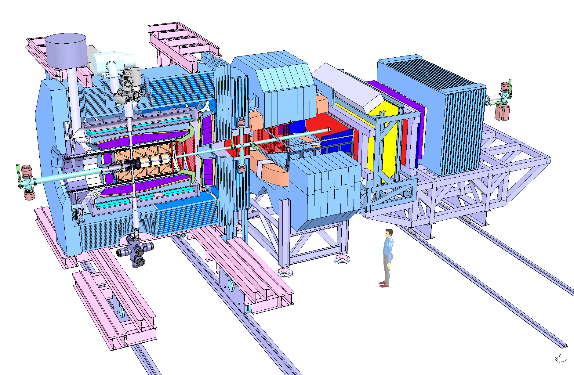
Figure 1: Schematic layout of the proposed Experiment at . The antiproton beam enters the detector from the left. The Target Spectrometer is complemented by a Forward Spectrometer to ensure full phase space coverage.

One obtains the maximum acceptance for the physics channels of interest when placing the detector system around a target internal to the ring that stores the antiprotons. Experimentally, this is a challenge. Antiproton beams of superior quality and intensity are difficult to produce. Although will provide the best anti-proton beams worldwide, its intensity will still be low compared to conventional particle beams. An appropriate target technology has to be developed to achieve high luminosity. Studying the decay of charmed particles requires a precise micro-vertex tracking detector system close to the interaction region as well as a powerful particle identification system. The latter should be able to discriminate hadron species as well as providing an excellent hadron/electron separation and muon identification. A central tracker will provide charged particle tracking. The Target Spectrometer detector system will be completed by a high-resolution electromagnetic calorimeter. A large solid angle coverage will be achieved by adding a Forward Spectrometer of similar capabilities. This complex detector arrangement will ensure the measurement of complete sets of observables, thus enabling to reach its physics goals.

Large Aperture Magnetic Spectrometers

The detection concept for the experiment is based on the reconstruction of charged particle tracks in magnetic fields in conjunction with calorimetry for neutral particles and muons. Only with this combination it will be possible to identify the reaction channels of interest unambiguously. The Target Spectro meter (TS) will consist of a superconducting solenoid, which will feature a 1.9 m free inner diameter to house a variety of tracking, particle identification and calorimetric detectors. The large-aperture resistive dipole magnet plus a set of analogous detectors will constitute the Forward Spectrometer (FS).

The Target Spectrometer will be the central part of the detector, and will enclose the interaction point. The solenoid magnet must provide a field of 2 T in the central region, where the trackers will be located, with a homogeneity of $\pm 2$% and very small radial field components, so that a 1.5 m long Time Projection Chamber (TPC) can be operated reliably. This translates to the requirement that the integral of the radial component along the $z$ axis $\int B_{r}(z)/B_{0}dz$ from any point inside the tracker to the read-out plane of the TPC must be less than 2 mm. At this level of precision the field is strongly dependent on many parameters, like details of the yoke geometry and coil arrangement, which in turn influence the design of several critical detectors inside the solenoid. Above requirements called for an extensive optimisation process in designing the solenoid, with many iterations.

For the TS magnet we chose to use a superconducting coil. The TS design is based on an aluminium stabilised, indirectly cooled superconducting solenoid using internal winding in an aluminium alloy mandrel. Aluminium stabilised cables give high stability against quenches due to the large electrical conductivity of aluminium at low temperature. The coil cable will withstand large thermal perturbations (energy releases) before a normal conducting zone starts to grow, leading to a quench. In addition, when a quench occurs it spreads more evenly than in other cable types, thus reducing high thermal stresses which could potentially lead to damages to the magnet.

By using internal winding, the cable will be pressed against the outer mandrel keeping to a minimum the stress on the epoxy glass insulation. Internal winding and indirect cooling will greatly reduce the amount of liquid helium, the cryostat design will be simplified and, since there will be no liquid helium bath, no pressure vessel will be needed. The helium will be contained in standard aluminium pipes rated to the maximum pressure that occurs during a quench or a major failure of the refrigerator. The use of internal winding and aluminium stabilised cables has been the technology chosen for many 4$\pi$ spectrometer solenoids from Cello in the early 80s to CMS at LHC today.

All detectors of the Target Spectrometer will be accommodated inside the solenoid, most of them inside the bore of the cryostat. This is a challenge for the design of the detectors, of their supports and supplies, and the magnet itself. A particular challenge is the accommodation of the target, which requires a vertical pipe traversing the magnet upstream of its centre. Consequently, the coil will be divided into three sub-coils, which renders the design of the coil former and of the cryostat much more difficult than those of other solenoid magnets. The target pipe will pass in between the first two sub-coils through a warm bore in the cryostat. The iron of the flux return yoke of the solenoid will act as an active muon range system. This is to be achieved by segmenting the yoke into 13 iron layers in the barrel and 5 iron layers in the downstream end cap interleaved with Mini Drift Tubes (MDTs).

It will be possible to open the flux return yoke from both upstream and downstream sides by sliding doors to give access to all detectors inside the solenoid. The whole TS, with all detectors in place, was designed to be movable from the in-beam position to a maintenance position.

Extensive studies regarding the electrical and mechanical properties of the solenoid were performed. Stresses and temperature gradients in the coil were analysed in detail. A quench protection system was designed and the behaviour of the coil during a quench was evaluated. Detailed Finite Element Model (FEM) calculations for the coil, cryostat, flux return yoke and support structures showed that all parts can be safely operated. Field studies showed that all fields fulfil the given requirements; and a powering and emergency shut-down procedure was developed.

The main purpose of the Forward Spectrometer is to reconstruct particles emitted from the target at angles below $5^{\circ}$ vertically and $10^{\circ}$ degrees horizontally. The large aperture resistive dipole magnet will provide a field integral of 2 Tm, allowing for a momentum reconstruction of charged particles to a precision of better than 1%. The dipole will have an aperture of about $1\times 3\,$m² to cover the aforementioned angular acceptance at about 3.5 m downstream from the interaction point. Inside this gap, two large tracking chambers and scintillation counters will be housed on a dedicated support frame which will allow their retraction for maintenance. In addition, support structures were designed, which will allow to mount the drift chambers at the entrance and exit of the dipole. The remaining detectors of the FS will be mounted on a platform that can be moved by a drive system from the maintenance and assembly position in the hall to the in-beam position. Between the TS solenoid and the FS dipole 5 instrumented layers of iron will add to the muon detection system and will decouple the magnetic fields of the solenoid and the dipole.

The decision to use resistive race-track coils for the dipole magnet was taken after evaluating alternative options in great detail. This choice proved to be the safest and most economic option both with respect to the investment as well as the running costs. The design was optimised to satisfy the requirements concerning the bending power, field homogeneity and acceptance providing sufficient space for the tracking detectors in the gap. A thorough mechanical analysis of the coil and frame stability was carried out. Extensive field studies showed that the bending of tracks traversing the magnet on different trajectories will vary no more than 10%. This can easily be handled by the track reconstruction software of . Since the dipole magnet will be part of the HESR lattice, its current must increase during the acceleration of antiprotons. Therefore the magnet was designed to ramp the current from 25% to 100% of its maximum value within 60 s. It was shown that a lamination of 20 cm is enough to keep the eddy currents at an acceptable level.

The design of the two large spectrometer magnets plus their support structures has been performed in a collaborative effort by seven groups from Germany, Italy, Poland, Russia and the UK. In Table 5.1, the institutes leading the design of specific items are listed.

• Coil and cryostat of the TS solenoid – INFN, Genoa.

• Instrumented flux return yoke of the TS solenoid – JINR, Dubna.

• Large aperture FS dipole magnet – University of Glasgow.

• Support structures for the FS detectors – CUT and UJ, Krakow.

• Rail systems and movement of the TS and the FS detector platform – GSI, Darmstadt and CUT, Krakow.

The Forschungszentrum Jülich (FZJ) takes care of the spectrometers’ integration into the HESR, which is particularly important for the dipole, since it will be part of the accelerator/storage ring lattice. A detailed list of institutions and work packages can be found in Chapter 5.

Both spectrometer magnets will act as mounting structures for the detectors. Therefore the two magnets will need to be in place before any mounting of the detectors can be started. We have taken this into account regarding the timelines, which foresee that all magnet components will be shipped to Darmstadt in 2012.

Chapter 1 Introduction

I. Lehmann

The physics of strong interactions is undoubtedly one of the most challenging areas of modern science. Quantum Chromo Dynamics (QCD) is reproducing the physics phenomena only at distances much shorter than the size of the nucleon, where perturbation theory can be used yielding results of high precision and predictive power. As the coupling constant rises steeply at nuclear scales (see Fig. 1.1) perturbative expansions diverge and a different theoretical approach is required. However, the strong interaction keeps providing new experimental observations, which were not predicted by “effective” theories. The latter retain the fundamental symmetries of QCD, but have problems in describing all the observed phenomena simultaneously.

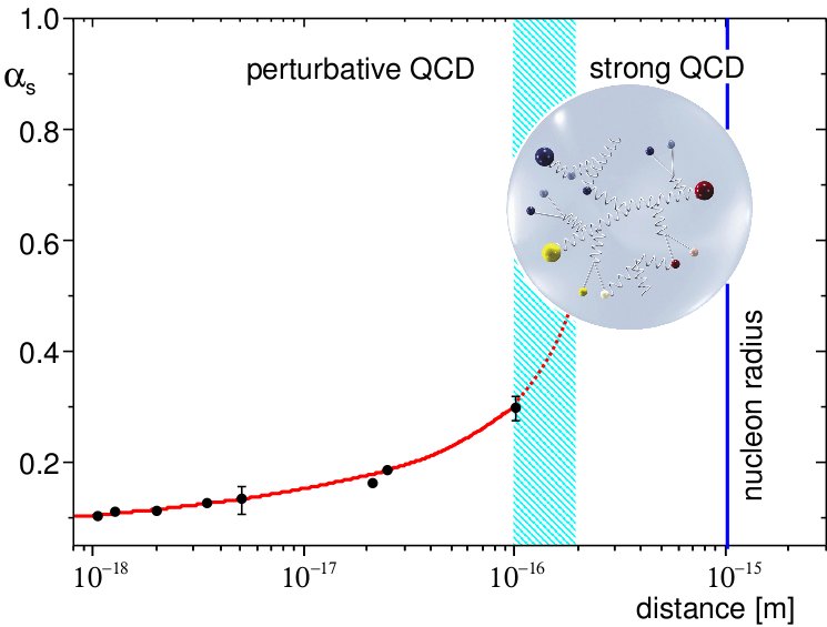
Figure 1.1: Coupling constant of the strong interaction as a function of distance. The data points represent experimental values [PDG2004]. For distances between quarks comparable to the nucleon size the interaction becomes so strong that quarks cannot be further separated (confinement) and hadrons are formed. will investigate the properties of the strong interaction in this key region for the understanding of matter.

The physics of strange and charmed quarks holds the potential to connect the two different energy domains interpolating between the limiting scales of QCD. In this regime only scarce experimental data are available, most of which have been obtained with electromagnetic probes.

One possible single issue that may greatly advance our understanding of hadronic structure is the predicted existence of states outside of the two- and three-quark classifications, which for example could arise from the excitation of gluonic degrees of freedom. Recent findings from running experiments at B-factories (see e.g. Refs [Acosta:2003zx, Choi:2003ue]) show that, indeed, unexpected narrow states unaccounted for in the naïve quark models exist. Experiments focused on the abundant production and systematic studies of these states are needed. Preferably, these should be performed using hadronic probes because the cross sections are expected to be very large in such systems. Results of high precision are a decisive element to be able to identify and extract features of these exotic states. Hadron beams are advantageous also for the production of hadrons with non-exotic quantum numbers, as these can be formed directly with high cross sections. Phase space cooling of the antiproton beam furthermore allows high precision determination of the mass and width of such states. Using heavier nuclei as targets enables us to investigate in-medium properties of hadrons and to produce hypernuclei, even those containing more than one strange quark, copiously.

The (Antiproton Annihilation at Darmstadt) experiment (see also Sec. 2 and Refs. [PANDA:TPR, PANDA:Intro]), which will be installed at the High Energy Storage Ring for antiprotons of the upcoming Facility for Antiproton and Ion Research (FAIR) [FAIR:BTR], features a scientific programme devoted to the following key areas.

• Charmonium spectroscopy.

• Search for gluonic excitations (hybrids and glueballs).

• Multi-quark states.

• Open and hidden charm in nuclei.

• Open charm spectroscopy.

• Hypernuclear physics.

• Electromagnetic processes.

These and selected further topics will be studied with unprecedented accuracy.

1.1 Topics Addressed at

Figure 1.2: Mass range of hadrons that will be accessible at PANDA. The upper scale indicates the corresponding antiproton momenta required in a fixed-target experiment. The HESR will provide 1.5 to 15 GeV/c antiprotons, which will allow charmonium spectroscopy, the search for charmed hybrids and glueballs, the production of D meson baryon pairs for pairs and the production of hypernuclear studies.

In the following major physics topics are briefly introduced. See also Fig. 1.2 for an overview. A detailed discussion and further references can be found in Ref. [PANDA:PhysBooklet].

Charmonium Spectroscopy.

The $\ccbar$ spectrum is often referred to as the positronium of QCD, because the properties of the states can be calculated precisely within the framework of non-relativistic potential models. More recently, results from quenched Lattice QCD emerged describing the known spectrum rather well. Recent findings of states around 4 $\gevc$ (X(3872), Z(3931), X(3940), Y(3940), Y(4260), Y(4320), to name only a few) [RBES1, RBES2, Z3931, X3940] show that the spectrum, which was believed to be well understood, in fact yields much more than has been expected.

will not only be able to measure those states in a different production channel, which may reveal more unexpected states, but also allow for scans over the width of those states with a precision of $10^{-5}$ relative to its mass. This is because one can produce these states directly in formation and make use of the precisely determined antiproton momenta in . At full luminosity will be able to collect several thousand $\ccbar$ states per day. Thus properties and branching ratios will be determined to a unprecedented precision.

Search for Gluonic Excitations (Hybrids and Glueballs).

One of the main challenges of hadron physics is the search for gluonic excitations, i.e. hadrons in which the gluons can act as principal components. In other words, the state cannot be fully described in terms of quantum numbers by solely taking its valence-quark content into account. These gluonic hadrons fall into two main categories described in the following. Glueballs are states where only gluons contribute to the overall quantum numbers while hybrids consist of a valence quarks as in ordinary hadrons plus one or more gluons which contribute to the overall quantum numbers.

The additional degrees of freedom carried by gluons allow these hybrids and glueballs to have $J^{PC}$ exotic quantum numbers. In this case mixing effects with nearby $\qqbar$ states are excluded and this makes their experimental identification easier. The properties of glueballs and hybrids are determined by the long-distance features of QCD and their study will yield fundamental insight into the structure of the QCD vacuum. Antiproton-proton annihilations provide a very favourable environment to search for gluonic hadrons.

Multi-Quark States.

These are states which cannot be assigned to an arrangement of tree quarks or a quark-antiquark pair as the classical baryons and mesons. Similarly to the gluonic excitations mentioned above they would show up as states outnumbering the multiplets and their clearest signature would be possible exotic quantum numbers. They could be interpreted as hadronic molecules or octet couplings. The well known states $a_{0}(980)$ and $f_{0}(975)$ are suspected to have admixtures of $K\bar{K}$ components. Here, however, mixing is large and clear statements on their nature are difficult to draw. In the charmonium region all states are narrower and positive identification is much more likely. This can also be seen from the current discussion on the nature of the X(3872) and other states recently found at the B-factories [RBES1, RBES2].

Open and Hidden Charm in Nuclei.

The study of medium modifications of hadrons embedded in hadronic matter is aimed at understanding the origin of hadron masses in the context of spontaneous chiral symmetry breaking in QCD and its partial restoration in a hadronic environment [Brown:1994cq]. So far experiments have been focused on the light quark sector. The high-intensity $\pbar$ beam of up to 15 GeV/c will allow an extension of this programme to the charm sector both for hadrons with hidden and open charm. The in-medium masses of these states are expected to be affected primarily by the gluon condensate.

Another study which can be carried out in PANDA is the measurement of $\jpsi$ and D meson production cross sections in $\pbar$ annihilation on a series of nuclear targets. The comparison of the resonant $\jpsi$ yield obtained from $\pbar$ annihilation on protons and different nuclear targets allows to deduce the $\jpsi$-nucleus dissociation cross section, a fundamental parameter to understand $\jpsi$ suppression in relativistic heavy ion collisions interpreted as a signal for quark-gluon plasma formation.

Open Charm Spectroscopy.

The HESR running at full luminosity and at $\pbar$ momenta larger than 6.4 GeV/c would produce a large number of $D$ meson pairs. The high yield (e.g. up to 100 charm pairs per second around the $\psi$(4040)) and the well defined production kinematics of $D$ meson pairs will allow to carry out a significant charmed meson spectroscopy programme which will include, for example, the rich $D$ and $D_{s}$ meson spectra.

Hypernuclear Physics.

Hypernuclei are systems in which up or down quarks are replaced by strange quarks. In this way a new quantum number, strangeness, is introduced into the nucleus. Although single and double $\Lambda$-hypernuclei were discovered many decades ago, only 6 events of double $\Lambda$-hypernuclei were observed up to now. The availability of $\pbar$ beams at FAIR will allow efficient production of hypernuclei with more than one strange hadron, making PANDA competitive with planned dedicated facilities. This will open new perspectives for nuclear structure spectroscopy and for studying the hyperon-nucleon and in particular the hyperon-hyperon interaction.

Electromagnetic Processes.

In addition to the spectroscopic studies described above, will be able to investigate the structure of the nucleon using electromagnetic processes, such as Wide Angle Compton Scattering (WACS) and the process $\pbarp\to\ee$, which will allow the determination of the electromagnetic form factors of the proton in the time-like region over an extended $q^{2}$ region. In addition the Drell-Yan process will allow to access the transverse nucleon spin structure.

1.2 Experimental Approach

Conventional as well as exotic hadrons can be produced by a range of different experimental means. Among these, hadronic annihilation processes, and in particular antiproton-nucleon and antiproton-nucleus annihilations, have proven to possess all the necessary ingredients for fruitful harvests in the hadron field.

• Hadron annihilations produce a gluon-rich environment, a fundamental prerequisite to copiously produce gluonic excitations.

• The use of antiprotons permits to directly form all states with non-exotic quantum numbers (formation experiments). Ambiguities in the reconstruction are reduced and cross sections are considerably higher compared to producing additional particles in the final state (production experiments). The appearance of states in production but not in formation is a clear sign of exotic physics.

• Narrow resonances, such as charmonium states, can be scanned with high precision in formation experiments using the small energy spread available with antiproton beams (cooled to $\Delta p/p=10^{-5}$).

• Since exotic systems will appear only in production experiments the physics analysis of Dalitz plots becomes important. This requires high-statistics data samples. Thus, high luminosity is a key requirement. This can be achieved using an internal target of high density, large numbers of projectiles and a high count-rate capability of the detector. The latter is mandatory since the overall cross sections of hadronic reactions are large while the cross sections of reaction channels of interest may be quite small.

• As reaction products are peaked around angles of $0^{\circ}$ a fixed-target experiment with a magnetic spectrometer is the ideal tool. At the same time a $4\pi$ coverage is mandatory to be able to study exclusive reactions with many decay particles. The physics topics as summarised in Fig. 1.2 confirm that the momentum range of the antiproton beam should extend up to 15 GeV/c with luminosities in the order of $10^{32}\,$cm^-2s^-1

To take full advantage of the HESR beam features, a compact, high resolution and high angular coverage spectrometer was designed. To cope with the need of $2\unit{Tm}$ bending power both at a very wide angular range in the laboratory reference frame, two magnets are necessary. A solenoid magnet provides the required bending power for particles exiting at $5-140^{\circ}$ in vertical direction and at $10-140^{\circ}$ in horizontal direction, whereas a dipole magnet provides bending power for particles exiting at angles smaller than $5^{\circ}$ in vertical direction and $10^{\circ}$ in horizontal direction. The requirements for both magnets are discussed in Sec. 2.4, the superconducting solenoid magnet is described in detail in Chapter 3 and the dipole magnet is described in Chapter 4.

Chapter 2 Spectrometer Overview

A. Bersani, I. Lehmann, R. Parodi, A. Vodopianov, G. Rosner

This chapter introduces the facility and the storage ring at which the experiment will be located. A brief overview over the detector and its components is given before concluding with the requirements which are imposed specifically to the two large spectrometer magnets in Sec. 2.4.

2.1 Facility for Antiproton and Ion Research –

The Facility for Antiproton and Ion Research () will be an accelerator facility leading the European research in nuclear and hadron physics in the coming decade. It will address a wide range of physics topics in the fields of nuclear structure, nuclear matter, studies using high energy and very slow antiprotons, atomic and plasma physics. Several topics in applied science and accelerator development will be addressed as well. builds on the experience and technological developments from the existing facility, and incorporates new technological concepts. In this document we briefly summarise aspects relating to the production of antiprotons for the use by the experiment. Please refer to Refs. [FAIR:BTR, FAIR:Info] for more details.

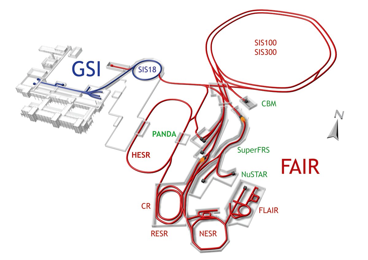
Figure 2.1: Layout of the facility. Shown are: synchrotrons with bending powers up to 18, 100 and 300 Tm the SIS 18, 100 and 300, respectively; the Collector Ring CR; the Accumulator Ring RESR; the low and high energy experimental storage rings NESR and HESR, respectively; and the Fragment Separator FRS.

The existing accelerators will be upgraded by the addition of a proton-linac and used as injectors for the newly built complex of storage rings to form the facility. An overview of the layout is given in Fig. 2.1. To the left, the existing facility is shown. New proposed beam lines and accelerator structures are shown in red. This facility will provide intense secondary beams of antiprotons and rare isotopes which will be used for research at the main experimental setups labelled in green.

will make use of antiprotons, which will be produced as follows. Protons will be accelerated to 70 MeV in a new linear accelerator and injected in several turns into the existing synchrotron SIS18 and accelerated to 2 GeV with a repetition rate of 5 Hz. After four SIS18 cycles and subsequent transfers to the SIS100 synchrotron, the protons will be accelerated to 29 GeV with a ramp rate of 4 T/s. Up to $2\times 10^{13}$ protons will be compressed into a single short bunch of less than 50 ns length in order to minimise the heating in the antiproton production target. The proton bunch will be directed onto a nickel target of about 60 mm length followed by a magnetic horn. The cycle of proton acceleration will be repeated every 10 s. (An upgrade allowing for a cycle time of 5 s is foreseen.) This scheme is expected to produce a bunch of at least $1\times 10^{8}$ antiprotons in the phase space volume which can be accepted by the magnetic separator and the Collector Ring (CR). The CR will be used for pre-cooling of the antiprotons. Thereafter, the antiprotons will be moderately compressed to a single bunch and transferred to the RESR storage ring. The antiprotons will be accumulated to high intensities in the RESR by a dedicated stochastic cooling system with a rate that matches the speed of cooling in the CR. The antiprotons will then be transferred at a momentum of 3.8 GeV/c to the High Energy Storage Ring (), which hosts and will be discussed in detail in the following.

2.2 High Energy Storage Ring –

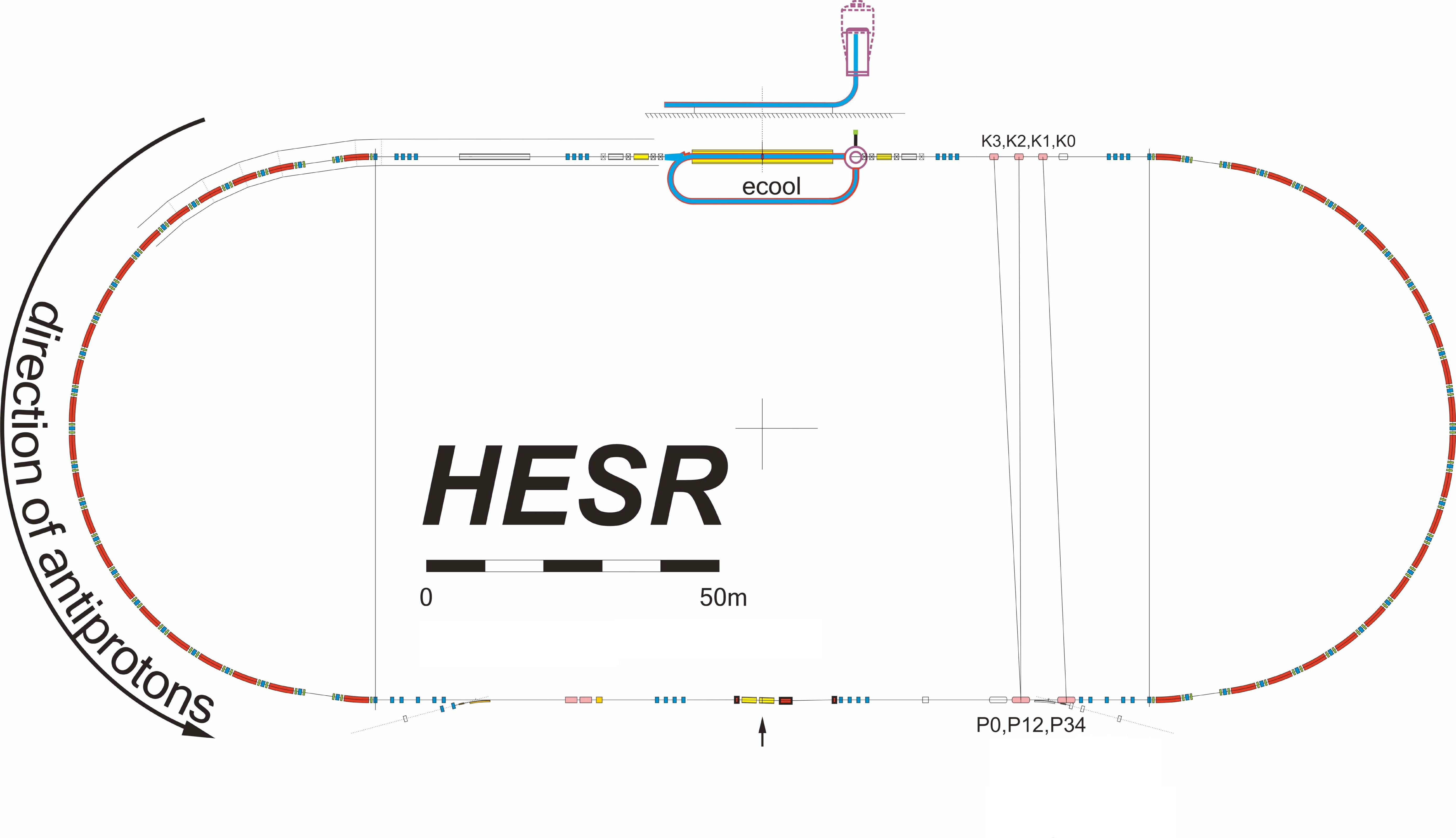
Figure 2.2: Layout of the High Energy Storage Ring . The following colour code is used for the active components: dipole magnets – red, quadrupoles – blue, solenoids – yellow, and cavities, pickups, kickers and septa – rosé or grey. The beam is injected into the lower straight section. Stochastic cooling ($P0-4$ and $K0-3$) and electron cooling (“ecool”) is foreseen. The location of the target is indicated with an arrow at the bottom of the figure. A detail of this section is shown in Fig. 2.15 later in this document.

The is dedicated to supply with high-quality anti-proton beams over a broad momentum range from 1.5 to 15 GeV/c. In storage rings the complex interplay of many processes like beam-target interaction and intra-beam scattering determines the final equilibrium distribution of the beam particles. Electron and stochastic cooling systems are required to ensure that the specified beam quality and luminosity for experiments at  [HESR:FAIR:2006, HESR:FAIR:2008] is achieved. Two different operation modes have been worked out to fulfil these experimental requirements. (Please also refer to Ref. [lehrach:stori:2008] and references therein.)

2.2.1 Lattice Design and Experimental Requirements

The lattice is designed as a racetrack shaped ring with a maximum beam rigidity of 50 Tm (see Fig. 2.2). The basic design consists of FODO cell structures in the arcs. The arc quadrupole magnets will be grouped into four families, to allow a flexible adjustment of transition energy, horizontal and vertical betatron tune, and horizontal dispersion.

One straight section will mainly be occupied by the electron cooler. The other straight section will host the experimental installation with internal H₂ pellet and cluster jet target, RF cavities, injection kickers and septa. Four stochastic cooling pickup and kicker tanks will also be located in the straight sections, opposite to each other.

Special requirements for the lattice are low dispersion in straight sections and small betatron amplitudes in the range between 1 and 15 m at the internal interaction point (IP) of the detector. In addition, the betatron amplitude at the electron cooler must be adjustable within a large range between 25 and 200 m. There are by now four defined optical settings: Injection, $\gamma_{tr}=6.2,\,\gamma_{tr}=13.4,\,\gamma_{tr}=33.2$. Both betatron tunes will roughly be 7.62 for different optical settings and natural chromaticities will be ranging in X from -12 to -17 and in Y from -10 to -13. Examples of the optical functions of the $\gamma_{tr}=6.2$ lattice are shown in Fig. 2.3.

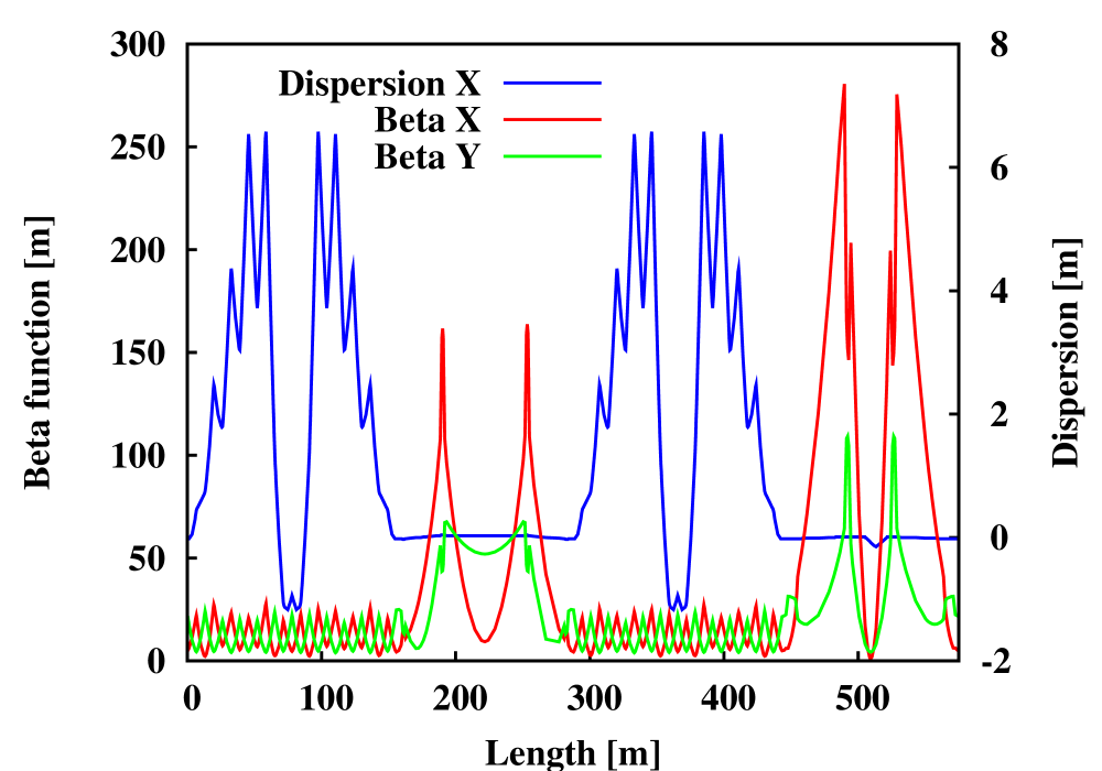
Figure 2.3: Optical functions of lattice for $\gamma_{tr}$ = 6.2 optical setting. Plotted are the horizontal dispersion, horizontal and vertical betatron function. The electron cooler is located at a length of $s$= 222 m, and the target at $s$=509 m, where a kink in the horizontal dispersion is generated by the dipole chicane.

The large aperture spectrometer dipole magnet also deflects the antiproton beam. To compensate for this two further dipole magnets surrounding the setup of the experiment will be used to create a beam chicane. To provide space for , the two chicane dipoles will be placed $4.6\unit{m}$ upstream and $13\unit{m}$ downstream the IP. This gives a boundary condition for the placement of the quadrupole elements closest to the experiment. For symmetry reasons, they have to be placed at $\pm 14\unit{m}$ with respect to the IP. The asymmetric placement of the chicane dipoles will result in the experiment axis occurring at a small angle with respect to the axis of the straight section.

Special equipment like multi-harmonic RF cavities, electron and stochastic cooler will enable a high performance of this antiproton storage ring to be achieved, and therefore make high precision experiments feasible. Key tasks for the design work to fulfil these requirements are:

Injection Parameters
Bunch length	150 m long bunches from RESR
Transverse emittance	0.25 mm $\times$ mrad (RMS) for $3.5\times 10^{10}$ particles,
	scaling with number of accumulated particles: $\sim N^{4/5}$
Relative momentum spread	$3.3\times 10^{-4}$ (RMS) for $3.5\times 10^{10}$ particles,
	scaling with number of accumulated particles: $\sigma_{p}/p\sim N^{2/5}$
Injection momentum	3.8 GeV/c
Injection type	Kicker injection using multi-harmonic RF cavities
Experimental Requirements
Ion species	Antiprotons
$\bar{p}$ production rate	$2\times 10^{7}$/s ($1.2\times 10^{10}$ per 10 min)
Momentum / Kinetic energy range	1.5 to 15 GeV/c / 0.83 to 14.1 GeV
Number of particles	$10^{10}$ to $10^{11}$
Target thickness	$4\times 10^{15}$atoms/cm2 (H2 pellets)
Beam size (radius) at IP	$\sim$ 1 mm (RMS)
Betatron amplitude at IP	1 – 15 m
Betatron amplitude E-Cooler	25 – 200 m
Operation Modes
High resolution (HR)	Peak Luminosity of 2$\times 10^{31}$cm-2 s-1 for $10^{10}\ \bar{p}$
	RMS momentum spread $\sigma_{p}/p\leq 4\times 10^{-5}$,
	1.5 to 9 GeV/c
High luminosity (HL)	Peak Luminosity up to 2$\times 10^{32}$cm-2 s-1 for $10^{11}\ \bar{p}$
	RMS momentum spread $\sigma_{p}/p\sim 10^{-4}$,
	1.5 to 15 GeV/c,

Table 2.1: Injection parameters, experimental requirements and operation modes.

• Design and testing of multi-harmonic RF cavities. One cavity is required for barrier-bucket operation to compensate the mean energy loss due to beam-target scattering. The second cavity is needed for bunch rotation, acceleration and deceleration of the beam. In addition, this second cavity will provide for bunch manipulation during refill to increase the average luminosity.

• Technical design study and prototyping of critical elements for high-voltage electron cooling system. An electron beam with up to 1 A current, accelerated in special accelerator columns to energies in the range of 0.4 to 4.5 MeV is planned for the HESR. The 24 m long solenoidal field in the cooler section has a longitudinal field strength of 0.2 T with a magnetic field straightness in the order of $10^{-5}$. This arrangement allows beam cooling between 1.5 GeV/c and 8.9 GeV/c. Since its design is modular, a future increase of high-voltage to 8 MV is possible, which would make electron cooling feasible in the whole HESR momenta range.

• Development and testing of high-sensitivity stochastic cooling pickups for the frequency range 2 – 4 GHz. The main stochastic cooling parameters have been determined for a cooling system utilising pickups and kickers with a band-width of 2 – 4 GHz and the option for an extension to 4 – 6 GHz. Since stochastic filter-cooling is specified above and stochastic time-of-flight cooling below 3.8 GeV/c, the whole HESR momentum range can be covered by the stochastic cooling system.

Table 2.1 summarises the specified injection parameters, experimental requirements and operation modes. Demanding requirements for high intensity and high quality beams are combined in two operation modes: high luminosity (HL) and high resolution (HR), respectively. The HR mode is defined in the momentum range from 1.5 to 9 GeV/c. To reach a relative momentum spread down to a few times $10^{-5}$, only $10^{10}$ circulating particles in the ring are anticipated. The HL mode requires an order of magnitude higher beam intensity with reduced momentum resolution to reach a peak luminosity of 2$\times 10^{32}$cm^-2 s^-1 in the full momentum range up to 15 GeV/c.

2.2.2 Beam Dynamics

Closed orbit correction

The most serious causes of closed orbit distortions are angular and spatial displacements of magnets. Alignment and measurement errors of beam position monitors also contribute to closed orbit distortions. Both types of errors have been included in the simulations.

The goal of the orbit correction scheme is to reduce maximum closed orbit deviations to below 5 mm while not exceeding 1 mrad of corrector strength. The inverted orbit response matrix method was utilised to obtain the necessary corrector strengths. In this simulation the correction scheme consists of 64 beam position monitors and 36 orbit correction dipoles. In order to verify the possibility to improve the closed orbit, Monte-Carlo methods have been used. More than 1000 different sets of displacement and measurement errors have been applied. For all defined optical settings the effectiveness of the developed closed orbit correction scheme could be demonstrated.

Additionally, the influence of the electron cooler toroids had to be investigated. Toroids are used in beam guiding systems of the electron cooler to overlap the electron beam with the antiproton beam. Since antiprotons are much heavier than electrons, the deflection of the antiprotons by toroids is much smaller. The deflection angles are different for the two transverse directions. To compensate this deflection four additional correction dipoles have to be included in the HESR lattice around the electron cooler. The inner ones need to be placed very close to the toroids to keep orbit deviations as small as possible.

There are a few positions in the straights of the HESR where orbit bumps will have to be used, e.g. at the target. Therefore, all closed orbit correction dipoles in the straights are designed to provide an additional deflection strength of 1 mrad. Investigations have shown that this is sufficient to set angle and position of the circulating beam in the desired ranges.

Beam momentum		1.5 GeV/c	9 GeV/c	15 GeV/c
Rel. loss rate $\tau_{loss}^{-1}$ $[$s${}^{-1}]$	Hadronic Interaction	$1.8\times 10^{-4}$	$1.2\times 10^{-4}$	$1.1\times 10^{-4}$
	Single Coulomb	$2.9\times 10^{-4}$	$6.8\times 10^{-6}$	$2.4\times 10^{-6}$
	Energy Straggling	$1.3\times 10^{-4}$	$4.1\times 10^{-5}$	$2.8\times 10^{-5}$
	Touschek Effect	$4.9\times 10^{-5}$	$2.3\times 10^{-7}$	$4.9\times 10^{-8}$
	Total	$6.5\times 10^{-4}$	$1.7\times 10^{-4}$	$1.4\times 10^{-4}$
Beam lifetime $t_{pbar}\;[$s$]$		$\sim 1540$	$\sim 6000$	$\sim 7100$
Max. luminosity $L_{max}$ $[10^{32}$cm-2 s${}^{-1}]$		0.82	3.22	3.93

Table 2.2: Upper limits for relative beam loss rate, beam lifetime ($1/e$) $t_{pbar}$, and maximum average luminosity $L_{max}$ for a H₂ pellet target.

Beam equilibria and luminosity estimates

Beam equilibria with electron cooling

The empirical magnetised cooling force formula by V.V. Parkhomchuk is generally used for electron cooling [parkhomchuk:2000], and an analytical description for intra-beam scattering [sorensen:1987]. Beam heating by beam-target interaction is described by transverse and longitudinal emittance growth due to Coulomb scattering and energy straggling [hinterberger:1989a, hinterberger:1989b]. Beam equilibria with electron cooled beams in the HESR have been investigated in detail [BoineFrankenheim:2006ci]. In the HR mode an RMS relative momentum spreads are ranging from $7.9\times 10^{-6}$ (1.5 GeV/c) to $2.7\times 10^{-5}$ (8.9 GeV/c), and $1.2\times 10^{-4}$ (15 GeV/c).

Beam equilibria with stochastic cooling

Beam equilibria have been simulated based on a Fokker-Planck approach. Applying stochastic cooling with a band-width of 2 – 6 GHz one can achieve an RMS relative momentum spread of $5.1\times 10^{-5}$ (3.8 GeV/c), $5.4\times 10^{-5}$ (8.9 GeV/c) and $3.9\times 10^{-5}$ (15 GeV/c) for the HR mode. In the HL mode RMS relative momentum spread of roughly $10^{-4}$ can be expected. Transverse stochastic cooling can be adjusted independently to ensure sufficient beam-target overlap.

The relative momentum spread can be further improved by combining electron- and stochastic cooling.

Beam losses and luminosity estimates

Beam losses are the main restriction for high luminosities. Three dominating contributions of beam-target interaction have been identified: Hadronic interaction, single Coulomb scattering at large angle and energy straggling of the circulating beam in the target. In addition, single intra-beam scattering due to the Touschek effect has also to be considered for beam lifetime estimates. Beam losses due to residual gas scattering can be neglected compared to beam-target interaction for a vacuum of $10^{-9}$ mbar. A detailed analysis of all beam loss processes in the HESR was carried out [lehrach:2006, hinterberger:2006].

The relative beam loss rate for the total cross section $\sigma_{tot}$ is given by the expression

$$\tau_{loss}^{-1}=n_{t}\sigma_{tot}f_{0}$$ (2.1)

where $\tau_{loss}^{-1}$ is the relative beam loss rate, $n_{t}$ the target thickness and $f_{0}$ the revolution frequency of the reference particle. In Table 2.2 calculated upper limits for beam losses and corresponding lifetimes are listed for transverse beam emittances of 1 mm$\times$mrad, betatron amplitudes of 1 m at the internal interaction point, a longitudinal ring acceptance of $\Delta p/p=\pm 10^{-3}$, and $10^{11}$ circulating antiprotons.

For beam-target interaction, the beam lifetime is calculated to be independent of the beam intensity, whereas for the Touschek effect it is found to depend on the beam equilibrium. Beam lifetimes ranging from 1540 s to 7100 s are found. Beam lifetimes at low momenta strongly depend on the beam cooling scenario and the ring acceptance. Less than half an hour beam lifetime is too small compared to the planned antiproton production rate.

The maximum average luminosity depends on the antiproton production rate $dN_{pbar}$ / dt = 2$\times 10^{7}$/s and loss rate

$$L_{max}=\frac{dN_{pbar}/dt}{\sigma_{tot}}.$$ (2.2)

Estimates of the maximum average luminosities are listed for different beam momenta in Table 2.2. The maximum average luminosity for 1.5 GeV/c is below the specified value for the HL mode.

Cycle averaged luminosity

To calculate the cycle averaged luminosity, machine cycles and beam preparation times have to be specified. After injection, the beam is pre-cooled to equilibrium (with target off) at 3.8 GeV/c. The beam is then accelerated or decelerated to the desired beam momentum. A maximum ramp rate of 25 mT/s is specified. After reaching the final momentum beam steering respectively focusing in the target and in beam cooler region will take place. Total beam preparation time $t_{prep}$ will range from 120 s for 1.5 GeV/c to 290 s for 15 GeV/c.

In the HL mode, particles should be re-used in the next cycle. Therefore the used beam will be converted back to the injection momentum and merged with the newly injected beam. A bucket scheme is planned for beam injection and refill procedure, utilising the second cavities. During acceleration 1% and deceleration 5% beam losses are assumed. The cycle averaged luminosity reads

$$\bar{L}=f_{0}N_{i,0}n_{t}\frac{\tau\left[1-e^{-t_{exp}/\tau}\right]}{t_{exp}+t_{prep}},$$ (2.3)

where $\tau$ is the $1/e$ beam lifetime, $t_{exp}$ the experimental time (beam on target time), and $t_{cycle}$ the total time of the cycle, with $t_{cycle}=t_{exp}+t_{prep}$. $N_{i,0}$ is the number of available particles after the target is switched on. The dependence of the cycle averaged luminosity on the cycle time is shown for different antiproton production rates in Fig. 2.4.

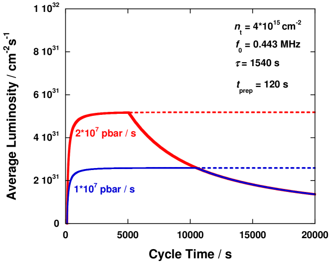
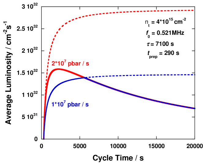
Figure 2.4: Cycle averaged luminosity vs. cycle time at 1.5 GeV/c (top) and 15 GeV/c (bottom). Assuming unlimited maximum number of particles inside the ring one obtains the dashed lines with a production rate of 1 or $2\times 10^{7}\bar{p}$/s (blue or red, respectively). In a more realistic scenario the number of particles which can be stored is limited to $10^{11}$ (solid lines).

With a limited number of antiprotons restricted to $10^{11}$, as specified for the HL mode, cycle averaged luminosities of up to 1.6$\times$ 10³²cm^-2s^-1 can be achieved at 15 GeV/c for cycle times of less than one beam lifetime. If one does not restrict the number of injected antiprotons, cycle times should be chosen longer to reach maximum average luminosities close to 3$\times$10³²cm^-2s^-1. This is a theoretical upper limit, since the larger momentum spread of the injected beam would lead to higher beam losses during injection due to limited longitudinal ring acceptance. Due do short beam lifetimes, more than $10^{11}$ particles can not be provided at the lowest momentum. This means that, at low momenta, cycle averaged luminosities are expected to be below 10³²cm^-2s^-1.

2.3 The Detector

The main objectives of the design of the experiment are to achieve $4\pi$ acceptance, high resolution for tracking, particle identification and calorimetry, high rate capabilities and a versatile readout and event selection. To obtain a good momentum resolution the detector will be composed of two magnetic spectrometers: the Target Spectrometer (TS), based on a superconducting solenoid magnet surrounding the interaction point, which will be used to measure at large angles and the Forward Spectrometer (FS), based on a dipole magnet, for small angle tracks. A silicon vertex detector will surround the interaction point. In both spectrometer parts, tracking, charged particle identification, electromagnetic calorimetry and muon identification will be available to allow to detect the complete spectrum of final states relevant for the physics objectives.

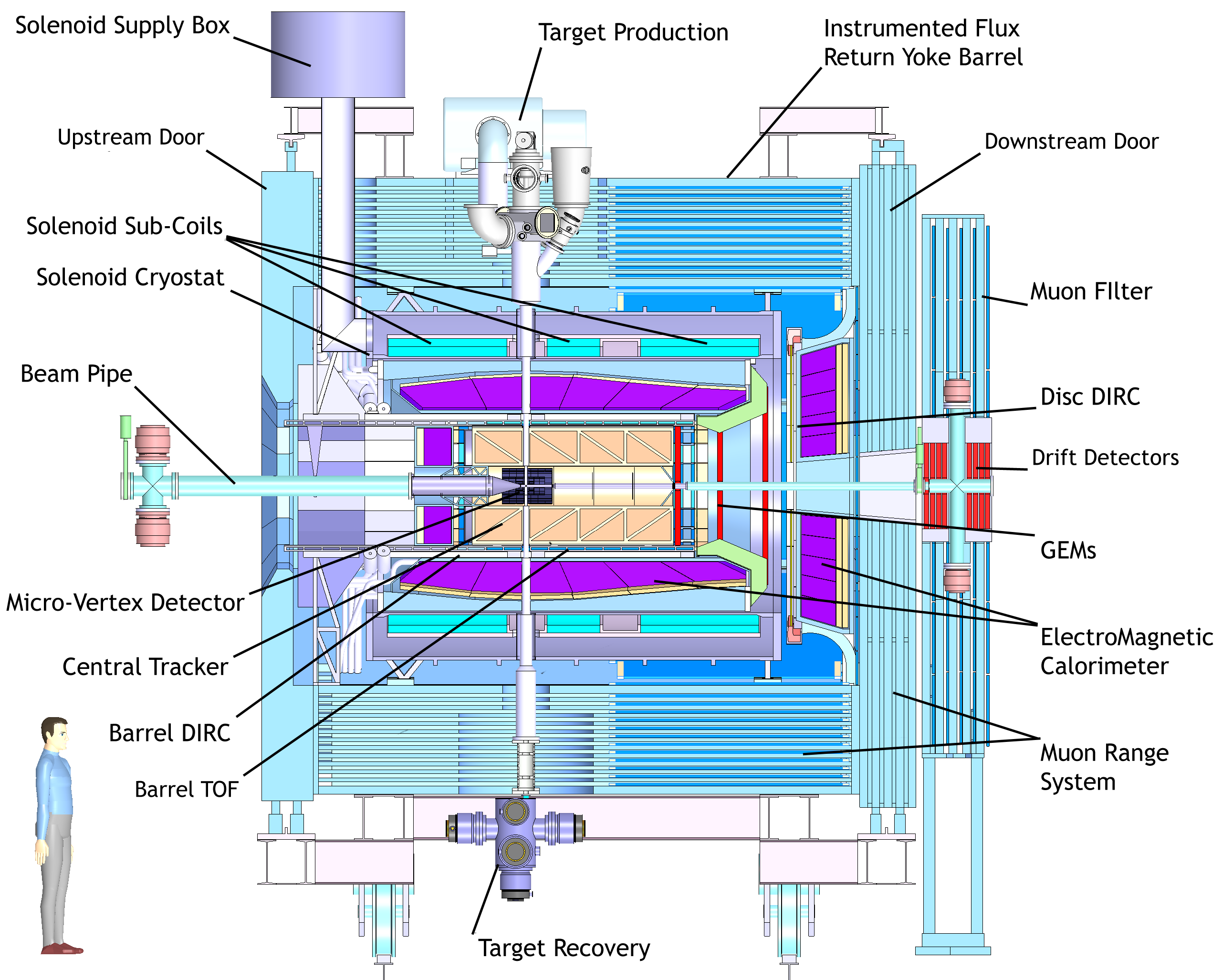
Figure 2.5: Artistic side view of the Target Spectrometer (TS) of . To the right of this the Forward Spectrometer (FS) follows, which is illustrated in Fig. 2.10.

2.3.1 Target Spectrometer

The Target Spectrometer will surround the interaction point and measure charged tracks in a highly homogeneous (better than $\pm$2%) solenoidal field of $2\unit{T}$. In the manner of a collider detector it will contain detectors in an onion shell like configuration. Pipes for the injection of target material will have to cross the spectrometer perpendicular to the beam pipe.

The Target Spectrometer will be arranged in three parts: the barrel covering angles between 22$\degrees$ and 140$\degrees$, the forward end cap extending the angles down to 5$\degrees$ and 10$\degrees$ in the vertical and horizontal planes, respectively, and the backward end cap covering the region between about 145$\degrees$ and 170$\degrees$. Please refer to Fig. 2.5 for an overview.

Target

The compact design of the detector layers nested inside the solenoidal magnetic field, combined with the request of minimal distance from the interaction point to the vertex tracker, leaves only a very restricted space for the target installations. In order to reach the design luminosity of $2\times 10^{32}$ s^-1cm^-2 a target thickness of about $4\times 10^{15}$ hydrogen atoms per cm² is required assuming $10^{11}$ stored anti-protons in the ring.

These conditions pose a real challenge for an internal target inside a storage ring. At present, two different, complementary techniques for the internal target are being developed further: the cluster-jet target and the pellet target. Both techniques are capable of providing sufficient densities for hydrogen at the interaction point, but exhibit different properties concerning their effect on the beam quality and the definition of the interaction point. In addition, internal targets also of heavier gases, like helium, deuterium, nitrogen or argon can be made available.

For non-gaseous nuclear targets the situation is different, in particular in the case of the planned hyper-nuclear experiment. In these studies, the whole upstream end cap and part of the inner detector geometry will be modified.

Cluster-Jet Target

The expansion of pressurised cold hydrogen gas into vacuum through a Laval-type nozzle leads to a condensation of hydrogen molecules forming a narrow supersonic jet of hydrogen clusters. The cluster size varies from $10^{3}$ to $10^{6}$ hydrogen molecules tending to become larger at higher inlet pressure and lower nozzle temperatures. Such a cluster-jet with density of $10^{15}$ atoms/cm² acts as a very diluted target since it may be seen as a localised and homogeneous monolayer of hydrogen atoms being passed by the antiprotons once per revolution.

Fulfilling the luminosity demand for still requires a density increase compared to current applications. Additionally, due to detector constraints, the distance between the cluster-jet nozzle and the target will be larger than usual. The great advantage of cluster targets is the homogeneous density profile and the possibility to focus the antiproton beam at highest phase space density. Hence, the interaction point is defined transversely but has to be reconstructed longitudinally in beam direction. In addition the low $\beta$-function of the antiproton beam keeps the transverse beam target heating effects at the minimum. The possibility of adjusting the target density along with the gradual consumption of antiprotons for running at constant luminosity will be an important feature.

Pellet Target

The pellet target features a stream of frozen hydrogen micro-spheres, called pellets, traversing the antiproton beam perpendicularly. Typical parameters for pellets at the interaction point are the rate of $1.0-1.5\times 10^{4}\unit{s^{-1}}$, the pellet size of $25-40\unit{\mu m}$, and the velocity of about 60 m/s. At the interaction point the pellet train has a lateral spread of $\sigma\approx 1\unit{mm}$ and an interspacing of pellets that varies between $0.5$ to $5\unit{mm.}$ With proper adjustment of the $\beta$-function of the coasting antiproton beam at the target position, the design luminosity for can be reached in time average. The present R&D is concentrating on minimising the luminosity variations such that the instantaneous interaction rate does not exceed the rate capability of the detector systems. Due to the large number of interactions expected in every pellet, and thanks to the foreseen pellet tracking system, a resolution in the vertex position of $50\unit{\mu m}$ will be possible with this target.

Other Targets

are under consideration for the hyper-nuclear studies where a separate target station upstream will comprise primary and secondary target and detectors. Moreover, current R&D is being undertaken for the development of a liquid helium target and a polarised ³He target. A wire target may be employed to study antiproton-nucleus interactions.

Solenoid Magnet

The magnetic field in the Target Spectrometer will be provided by a superconducting solenoid coil with an inner radius of $105\unit{cm}$ and a length of $2.8\unit{m}$. The maximum magnetic field needs to be $2\unit{T}$. The field homogeneity is foreseen to be better than $2\%$ over the volume of the vertex detector and central tracker. In addition the transverse component of the solenoid field should be as small as possible, in order to allow a uniform drift of charges in the time projection chamber. This is expressed by a limit of $\int B_{r}/B_{z}dz<2\unit{mm}$ for the normalised integral of the radial field component.

In order to minimise the amount of material in front of the electromagnetic calorimeter, the latter will be placed inside the magnetic coil. The tracking devices in the solenoid will cover angles down to $5\degrees{}/10\degrees{}$ where momentum resolution is still acceptable. The dipole magnet with a gap height of $1.4\unit{m}$ provides a continuation of the angular coverage to smaller polar angles.

The cryostat for the solenoid coils is required to have two warm bores of $100\unit{mm}$ diameter, one above and one below the target position, to allow for insertion of internal targets.

The proposed Target Spectrometer solenoid is comparable by dimensions and field to the solenoid built in the late eighties for the ZEUS experiment at HERA, the proton electron collider of the DESY laboratory at Hamburg.

The winding construction proposed for the solenoid is based on the well proven technique used for the superconducting coils used since the beginning of the eighties in the High Energy Physics and nuclear physics experiments. We propose to use the same technology used for superconducting solenoids like CELLO and ZEUS (DESY), ALEPH, DELPHI, ATLAS, CMS (CERN), BABAR (SLAC), CDF (FERMILAB), BELLE (KEK), FINUDA, KLOE (LNF_INFN).

Micro-Vertex Detector

The design of the micro-vertex detector () for the Target Spectrometer is optimised for the detection of secondary vertices from and hyperon decays and maximum acceptance close to the interaction point. It will also strongly improve the transverse momentum resolution. The setup is depicted in Fig. 2.6.

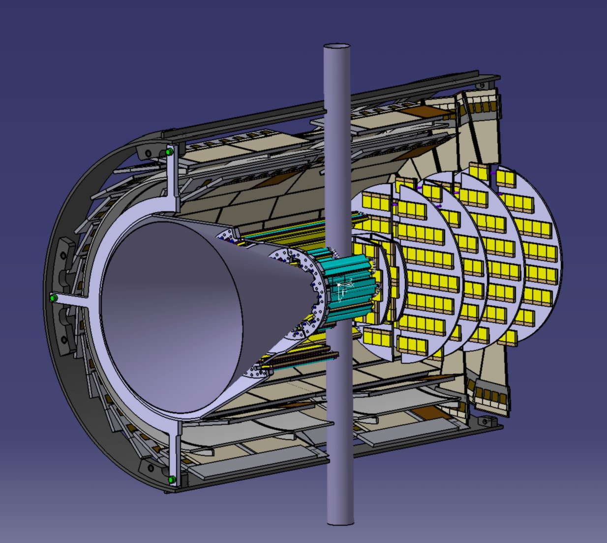
Figure 2.6: The Micro-Vertex Detector (MVD) of the Target Spectrometer surrounding the beam and target pipes seen from upstreams. The outer barrel layers are cut for visibility.

The concept of the is based on radiation hard silicon pixel detectors with fast individual pixel readout circuits and silicon strip detectors. The layout foresees a four layer barrel detector with an inner radius of $2.5\unit{cm}$ and an outer radius of $13\unit{cm}$. The two innermost layers will consist of pixel detectors and the outer two layers will consist of double sided silicon strip detectors.

Eight detector wheels arranged perpendicular to the beam will achieve the best acceptance for the forward part of the particle spectrum. Here again, the inner four layers will be made entirely of pixel detectors, the following two will be a combination of strip detectors on the outer radius and pixel detectors closer to the beam pipe. Finally the last two wheels, made entirely of silicon strip detectors, will be placed further downstream to achieve a better acceptance of hyperon cascades.

Central Tracker

The charged particle tracking devices must handle the high particle fluxes that are anticipated for a luminosity of up to several $10^{32}\,$cm^-2s^-1. The momentum resolution $\delta p/p$ has to be on the percent level. The detectors should have good detection efficiency for secondary vertices which can occur outside the inner vertex detector (e.g.  $\Ks$ or $\Lambda$). This will be achieved by the combination of the silicon vertex detectors close to the interaction point () with two outer systems. One system will cover a large area and is designed as a barrel around the . This will be either a stack of straw tubes () or a time-projection chamber (). The forward angles will be covered using three sets of GEM trackers similar to those developed for the COMPASS experiment at CERN. The two options for the central tracker are explained briefly in the following.

Straw Tube Tracker ()

This detector will consist of aluminised Mylar tubes called straws, which will be self supporting by the operation at $1\unit{bar}$ overpressure. The straws are to be arranged in planar layers which are mounted in a hexagonal shape around the as shown in Fig. 2.7. In total there are 24 layers of which the 8 central ones are tilted to achieve an acceptable resolution of $3\unit{mm}$ also in z (parallel to the beam). The gap to the surrounding detectors will be filled with further individual straws. In total there will be 4200 straws around the beam pipe at radial distances between 15 cm and 42 cm with an overall length of 150 cm. All straws have a diameter of $10\unit{mm}$. A thin and light space frame will hold the straws in place, the force of the wire however is kept solely by the straw itself. The Mylar foil is 30 $\mu$m thick, the wire is made of 20$\,\mu$m thick gold plated tungsten. This design results in a material budget of 1.3 % of a radiation length.

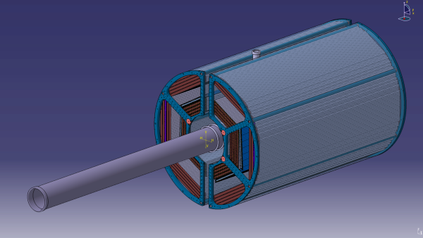
Figure 2.7: Straw Tube Tracker (STT) of the Target Spectrometer with beam and target pipes seen from upstreams.

The gas mixture used will be Argon based with CO₂ as quencher. It is foreseen to have a gas gain no greater than 10⁵ in order to warrant long term operation. With these parameters, a resolution in $x$ and $y$ coordinates of less than 150$\,\mu$m is expected.

Time Projection Chamber ()

A challenging but advantageous alternative to the is a , which would combine superior track resolution with a low material budget and additional particle identification capabilities through energy loss measurements.

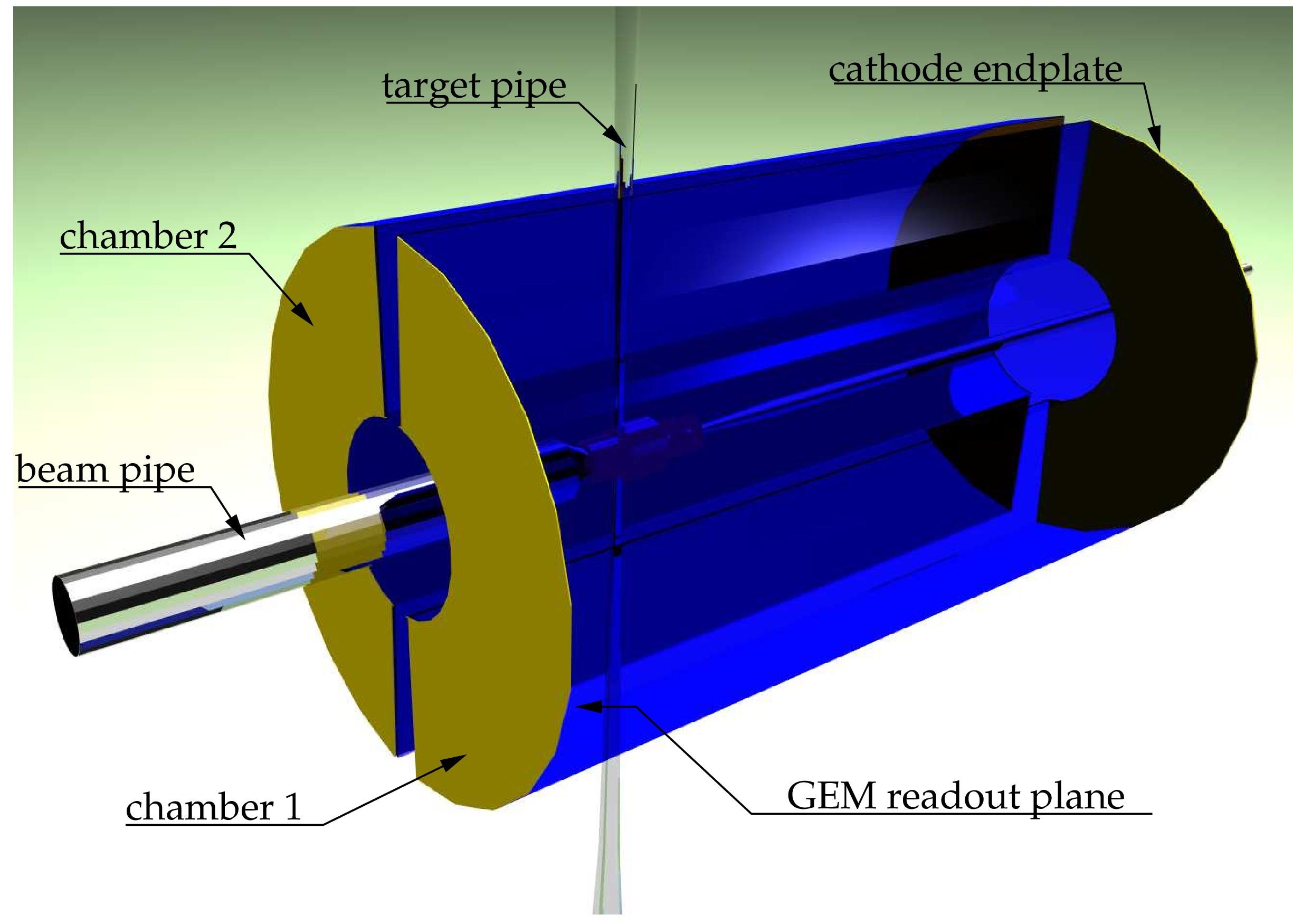
Figure 2.8: GEM Time Projection Chamber (TPC) of the Target Spectrometer with beam and target pipes seen from upstreams.

The planned depicted in a schematic view in Fig. 2.8 will consist of two large gas-filled half-cylinders enclosing the target and beam pipe and surrounding the . An electric field along the cylinder axis separates positive gas ions from electrons created by ionising particles traversing the gas volume. The electrons drift with constant velocity towards the anode at the upstream end face and create an avalanche detected by a pad readout plane yielding information on two coordinates. The third coordinate of the track comes from the measurement of the drift time of each primary electron cluster. In common TPCs the amplification stage typically occurs as in multi-wire proportional chambers. These are gated by an external trigger to avoid a continuous back flow of ions in the drift volume which would distort the electric drift field and jeopardise the principle of operation. In the interaction rate will be too high and there is no fast external trigger to allow such an operation. Therefore a novel readout scheme will be employed which is based on Gas Electron Multiplier (GEM) foils as amplification stage.

From the viewpoint of the solenoid magnet, the compatibility with the requires a very good homogeneity of the solenoid field with a low radial component. The solenoid magnet was designed, anyhow, to comply with the most stringent requirements coming from both solutions.

Forward GEM Detectors

Particles emitted at angles below 22 which are not covered fully by the Straw Tube Tracker or will be tracked by three stations of Gas Electron Multiplier (GEM) detectors placed 1.1 m, 1.4 m and 1.9 m downstream of the target. The chambers have to sustain a high counting rate of particles peaked at the most forward angles due to the relativistic boost of the reaction products as well as due to the small angle $\pbar$p elastic scattering. With the envisaged luminosity, the expected particle flux in the first chamber in the vicinity of the $5\unit{cm}$ diameter beam pipe will be about $3\times 10^{4}\,$cm^-2s^-1. Gaseous micro-pattern detectors based on GEM foils as amplification stages are chosen. These detectors have rate capabilities three orders of magnitude higher than drift chambers. In the current layout there will be three double planes with two projections per plane.

Cherenkov Detectors and Time-of-Flight

Charged particle identification of hadrons and leptons over a large range of angles and momenta is an essential requirement for meeting the physics objectives of . There will be several dedicated systems which, complementary to the other detectors, will provide means to identify particles. The main part of the momentum spectrum above 1 GeV/$c$ will be covered by Cherenkov detectors. Below the Cherenkov threshold of kaons several other processes have to be employed for particle identification. In addition a time-of-flight barrel will identify slow particles.

Barrel Time-of-Flight

For slow particles at large polar angles particle identification will be provided by a time-of-flight detector. In the Target Spectrometer the flight path is only in the order of 50 – 100 cm. Therefore the detector must have a very good time resolution between 50 and 100 ps.

As detector candidates scintillator bars and strips or pads of multi-gap resistive plate chambers are considered. In both cases a compromise between time resolution and material budget has to be found. The detectors will cover angles between 22 and 140 using a barrel arrangement around the /at 42 - 45 cm radial distance.

Barrel DIRC

At polar angles between 22 and 140, particle identification will be performed by the detection of internally reflected Cherenkov () light as realised in the BaBar detector [Staengle:1997xp]. It will consist of 1.7 cm thick fused silica (artificial quartz) slabs surrounding the beam line at a radial distance of 45 - 54  cm. At BaBar the light was imaged across a large stand-off volume filled with water onto 11 000 photomultiplier tubes. At , it is intended to focus the images by lenses onto micro-channel plate photomultiplier tubes (MCP PMTs) which are insensitive to magnet fields. This fast light detector type allows a more compact design and the readout of two spatial coordinates.

The DIRC design with its compact radiator mounted close to the will minimise the conversions. Part of these conversions will be recovered with information from the DIRC detector, as was shown by BaBar [Adametz05].

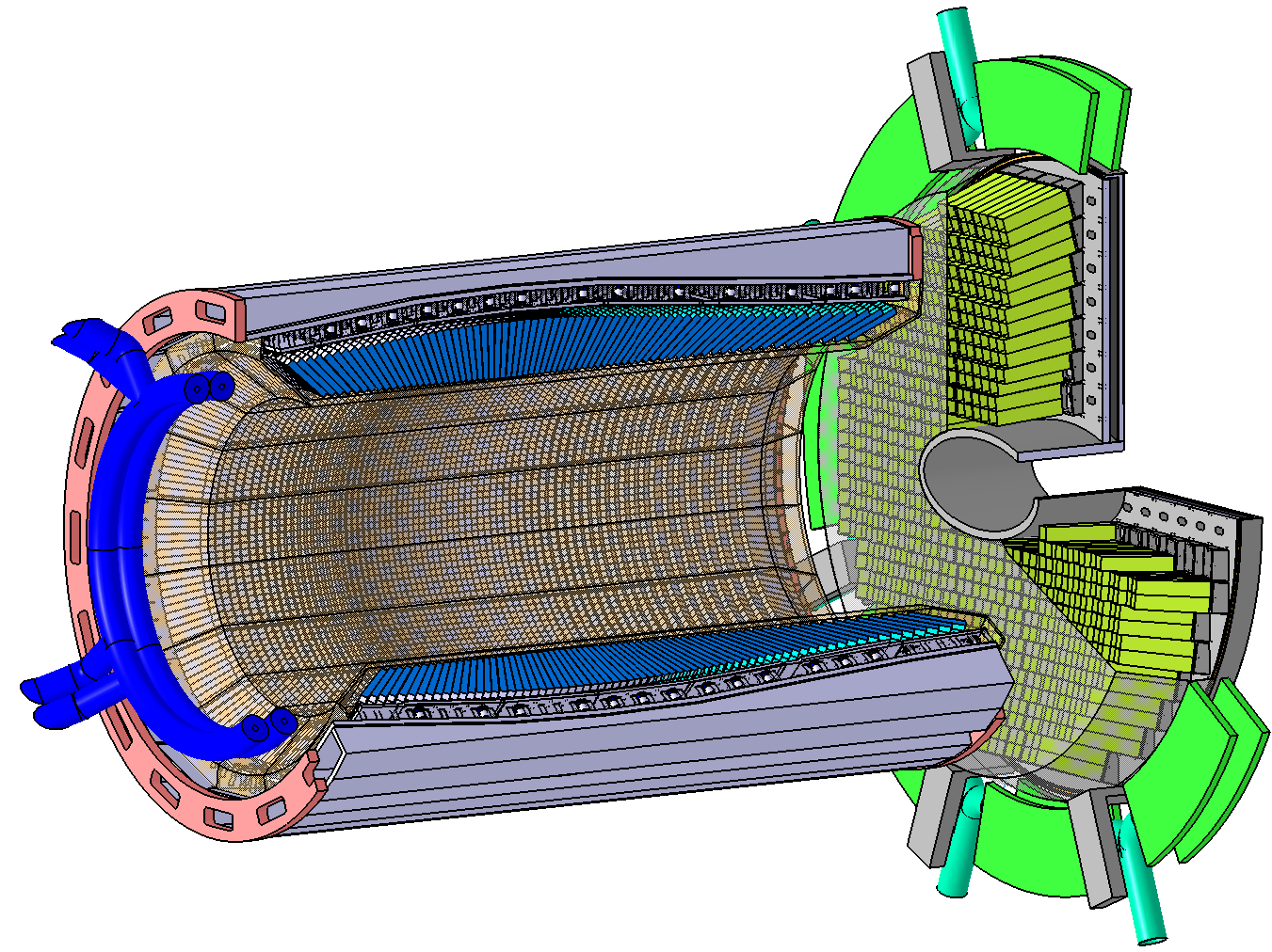
Figure 2.9: Barrel and forward end cap of the Electro-Magnetic Calorimeter (EMC) with its mounting structures and cooling pipes. These structures will be mounted directly inside the cryostat and forward end of the flux return yoke.

Forward End-Cap DIRC

A similar concept can be employed in the forward direction for particles between 5 and 22. The same radiator, fused silica, is to be employed however in shape of a disk. At the rim around the disk the Cherenkov angle will be measured either directly by focusing elements or indirectly using time-of-propagation (ToP). In the first option focusing will be done by mirroring quartz elements reflecting onto MCP PMTs. Once again two spatial coordinates plus the propagation time for corrections will be read. In the ToP design this angle is reconstructed by using the known path of the photon and its time of propagation. This will be achieved by the use of alternating dichroic mirrors transmitting and reflecting different parts of the light spectrum . The disk will be 2 cm thick and will have a radius of 110 cm. It will be placed directly upstream of the forward end cap calorimeter.

Electromagnetic Calorimeters

Expected high count rates and a geometrically compact design of the Target Spectrometer require a fast scintillator material with a short radiation length and Molière radius for the construction of the electromagnetic calorimeter (). Lead tungsten (PbWO₄) is a high density inorganic scintillator with sufficient energy and time resolution for photon, electron, and hadron detection even at intermediate energies [Mengel:1998si, Novotny:2000zg, Hoek:2002ss].

The crystals will be 20 cm long, i.e. approximately 22$\,X_{0}$, in order to achieve an energy resolution below 2 at 1$\,\gev$ [Mengel:1998si, Novotny:2000zg, Hoek:2002ss] at a tolerable energy loss due to longitudinal leakage of the shower. Tapered crystals with a front size of $2.1\times 2.1\,\cm^{2}$ will be mounted in the barrel EMC with an inner radius of 57 cm. This implies 11360 crystals for the barrel part of the calorimeter. The forward end cap EMC will be a planar arrangement of 3600 tapered crystals with roughly the same dimensions as in the barrel part, and the backward end cap EMC comprises of 592 crystals. The readout of the crystals will be accomplished by large area avalanche photo diodes in the barrel and vacuum photo-triodes in the forward and backward end caps. The light yield can be increased by a factor of about 4 compared to room temperature by cooling the crystals down to -25$\degC$. The arrangement of the barrel and forward end cap calorimeters is shown in Fig. 2.9.

The EMC will allow to achieve an e/$\pi$ ratio of 10³ for momenta above 0.5$\,\gevc$. Therefore, e-$\pi$-separation will not require an additional gas Cherenkov detector in favour of a very compact geometry of the EMC. For further details please refer to Ref. [PANDA:TDR:EMC].

Muon Detectors

In the barrel region the yoke is segmented and will consist of 13 layers in total: the innermost layer will have a thickness of 6 cm equal to the outermost one, in between 11 layers of 3 cm thickness will be located. The gaps for the detectors will be 3 cm wide. This is enough material for the absorption of pions in the momentum range in at these angles. In the forward end cap more material is needed. Since the downstream door of the return yoke has to fulfil constraints for space and accessibility, the muon system will split in several layers. Six detection layers will be placed around five iron layers of 6 cm each within the door, and a removable muon filter with additional five layers of 6 cm iron is located in the space between the solenoid and the dipole. This filter has to provide cut-outs for forward detectors and pump lines and has to be built in a way that it can be removed with few crane operations to allow easy access to these parts. The integration with the muon system was the most challenging requirement for the instrumented flux return yoke design.

As detector within the absorber layers rectangular aluminum drift tubes will be used as they were constructed for the COMPASS muon detection system. They are essentially drift tubes with additional capacitive coupled strips read out on both ends to obtain the longitudinal coordinate.

Figure 2.10: Artistic side view of the Forward Spectrometer (FS) of . It is preceded on the left by the Target Spectrometer (TS), which is illustrated in Fig. 2.5.

Hypernuclear Detector

The hypernuclei study will make use of the modular structure of . Removing the backward end cap calorimeter will allow to add a dedicated nuclear target station and the required additional detectors for $\gamma$ spectroscopy close to the entrance of . While the detection of anti-hyperons and low momentum $K^{+}$ can be ensured by the universal detector and its PID system, a specific target system and a $\gamma$-detector are additional components required for the hypernuclear studies.

Active Secondary Target

The production of hypernuclei proceeds as a two-stage process. First hyperons, in particular $\Xi\bar{\Xi}$, are produced on a nuclear target. In some cases the $\Xi$ will be slow enough to be captured in a secondary target, where it reacts in a nucleus to form a double hypernucleus.

The geometry of this secondary target is determined by the short mean life of the $\Xi^{-}$ of only 0.164 ns. This limits the required thickness of the active secondary target to about 25–30 mm. It will consist of a compact sandwich structure of silicon micro strip detectors and absorbing material. In this way the weak decay cascade of the hypernucleus can be detected in the sandwich structure.

Germanium Array

An existing germanium-array with refurbished readout will be used for the $\gamma$-spectroscopy of the nuclear decay cascades of hypernuclei. The main limitation will be the load due to neutral or charged particles traversing the germanium detectors. Therefore, readout schemes and tracking algorithms are presently being developed which will enable high resolution $\gamma$-spectroscopy in an environment of high particle flux.

2.3.2 Forward Spectrometer

The Forward Spectrometer (FS) will cover all particles emitted in vertical and horizontal angles below $\pm 5^{\circ}$ and $\pm 10^{\circ}$, respectively. Charged particles will be deflected by an integral dipole field of 2 Tm. Cherenkov detectors, calorimeters and muon counters ensure the detection of all particle types. Please refer to Fig. 2.10 for an overview.

Dipole Magnet

A 2 Tm dipole magnet with a window frame, a 1 m gap, and more than 2 m aperture will be used for the momentum analysis of charged particles in the Forward Spectrometer. In the current planning, the magnet yoke will occupy about 1.6 m in beam direction starting from 3.9 m downstream of the target. Thus, it covers the entire angular acceptance of the Target Spectrometer of $\pm$10 and $\pm$5 in the horizontal and in the vertical direction, respectively. The bending power of the dipole on the beam line causes a deflection of the antiproton beam at the maximum momentum of 15$\,\gevc$ of 2.2. The designed acceptance for charged particles covers a dynamic range of a factor 15 with the detectors downstream of the magnet. For particles with lower momenta, detectors will be placed inside the yoke opening. The beam deflection will be compensated by two correcting dipole magnets, placed around the detection system.

Forward Trackers

The deflection of particle trajectories in the field of the dipole magnet will be measured with three pairs of tracking drift detectors. The first pair will be placed in front, the second within and the third behind the dipole magnet. Each pair will contain two autonomous detectors as described below. Thus, in total, 6 independent detectors will be mounted. Each tracking detector will consist of four double-layers of straw tubes (see Fig. 2.11), two with vertical wires and two with wires inclined by a few degrees. The optimal angle of inclination with respect to vertical direction will be chosen on the basis of ongoing simulations. The planned configuration of double-layers of straws will allow to reconstruct tracks in each pair of tracking detectors separately, also in case of multi-track events.

Figure 2.11: Double layer of straw tubes with preamplifier cards and gas manifolds mounted on rectangular support frame. The opening in the middle of the detector is foreseen for the beam pipe.

Forward Particle Identification

RICH Detector

To enable the $\pi$/$K$ and $K$/p separation also at the highest momenta a detector is proposed. The favoured design is a dual radiator detector similar to the one used at HERMES [Akopov:2000qi]. Using two radiators, silica aerogel and C₄F₁₀ gas, provides $\pi$/$K$/p separation in a broad momentum range from 2 to 15$\,\gevc$. The two different indices of refraction are 1.0304 and 1.00137, respectively. The total thickness of the detector is reduced to the freon gas radiator (5%$\,X_{0}$), the aerogel radiator (2.8%$\,X_{0}$), and the aluminum window (3%$\,X_{0}$) by using a lightweight mirror focusing the Cherenkov light on an array of photo-tubes placed outside the active volume.

Time-of-Flight Wall

A wall of slabs made of plastic scintillator and read out on both ends by fast photo-tubes will serve as time-of-flight stop counter placed at about 7 m from the target. In addition, similar detectors will be placed inside the dipole magnet opening, to detect low momentum particles which do not exit the dipole magnet. With the expected time resolution of $\sigma\,=\,50\,$ps $\pi$/$K$ and $K$/p separation on a 3$\,\sigma$ level will be possible up to momenta of 2.8$\,\gevc$ and 4.7$\,\gevc$, respectively.

Forward Electromagnetic Calorimeter

For the detection of photons and electrons a Shashlyk-type calorimeter with high resolution and efficiency will be employed. The detection is based on lead-scintillator sandwiches read out with wave-length shifting fibres passing through the block and coupled to photo-multipliers. The technique has already been successfully used in the E865 experiment [bib:emc:E865] and it has been adopted for various other experiments like PHENIX and LHCb. An energy resolution of $4\%/\sqrt{E}$ [bib:emc:KOP99] has been achieved. A view of a 3x3 matrix of Shashlyk modules with lateral size of 110 mm x 110 mm and a length of 680 mm ($=\,20X_{0}$) is shown in Fig. 2.12. To cover the forward acceptance, 351 such modules arranged in 13 rows and 27 columns at a distance of 7.5 m from the target are required.

Figure 2.12: $3\times 3$ matrix of prototype Shashlyk modules as they should be employed for the Forward Electromagnetic Calorimeter.

Forward Muon Detectors

For the very forward part of the muon spectrum, a further range tracking system consisting of interleaved absorber layers and rectangular aluminium drift-tubes is being designed, similar to the muon system of the Target Spectrometer, but laid out for higher momenta. The system allows discrimination of pions from muons, detection of pion decays and, with moderate resolution, also the energy determination of neutrons and anti-neutrons. The forward muon system will be placed at about 9 m from the target.

2.3.3 Luminosity monitor

In order to determine the cross section for physical processes, it is essential to determine the time integrated luminosity $L$ for reactions at the interaction point that was available while collecting a given data sample. In the following we concentrate on elastic antiproton-proton scattering as the reference channel. For most other hadronic processes that will be measured concurrently in the precision is rather poor with which the cross sections are known.

The basic concept of the luminosity monitor is to reconstruct the angle of the scattered antiprotons in the polar angle range of 3-8 mrad with respect to the beam axis. Due to the large transverse dimensions of the interaction region when using the pellet target, there is only a weak correlation of the position of the antiproton at e.g. $z=+10.0$ m to the recoil angle. Therefore, it is necessary to reconstruct the angle of the antiproton at the luminosity monitor. As a result the luminosity monitor will consist of a sequence of four planes of double-sided silicon strip detectors located as far downstream and as close to the beam axis as possible. The planes are separated by 20 cm along the beam direction. Each plane consists of 4 wafers (e.g. 2 cm$\times$5 cm $\times\ 200\,\mu$m, with 50 $\mu$m pitch) arranged radially to the beam axis. Four planes are required for sufficient redundancy and background suppression. The use of 4 wafers (up, down, right, left) in each plane allows systematic errors to be strongly suppressed.

The silicon wafers will be located inside a vacuum chamber to minimize scattering of the antiprotons before traversing the 4 tracking planes. The luminosity monitor can be located in the space between the downstream side of the forward muon system and the HESR dipole needed to redirect the antiproton beam out of the chicane back into the direction of the HESR straight stretch (i.e.  between $z=+11$ m and $z=+13$ m downstream of the target).

As pilot simulations show, at a beam momentum of 6.2 GeV/$c$ the proposed detector measures antiprotons elastically scattered in the range $0.0006$(GeV)${}^{2}<-t<0.0035$ (GeV)², which spans the Coulomb-nuclear interference region. Based upon the granularity of the readout the resolution of $t$ could reach $\sigma_{t}\approx 0.0001$ (GeV)². In reality this value is expected to degrade to $\sigma_{t}\approx 0.0005$ (GeV)² when taking small-angle scattering into account. At the nominal interaction rate of $2\times 10^{7}$/s there will be an average of 10 kHz/cm² in the sensors. In comparison with other experiments an absolute precision of about 3% is considered feasible for this detector concept at , which will be verified by more detailed simulations.

2.3.4 Data Acquisition

In , a data acquisition concept is being developed to be as much as possible matched to the high data rates, to the complexity of the experiment and the diversity of physics objectives and the rate capability of at least $2\times 10^{7}$ events/s.

In our approach, every sub-detector system is a self-triggering entity. Signals are detected autonomously by the sub-systems and are preprocessed. Only the physically relevant information is extracted and transmitted. This requires hit-detection, noise-suppression and clusterisation at the readout level. The data related to a particle hit, with a substantially reduced rate in the preprocessing step, is marked by a precise time stamp and buffered for further processing. The trigger selection finally occurs in computing nodes which access the buffers via a high-bandwidth network fabric. The new concept provides a high degree of flexibility in the choice of trigger algorithms. It makes trigger conditions available which are outside the capabilities of the standard approach.

2.3.5 Infrastructure

The target for antiproton physics will be located in the straight section at the east side of the . At this location an experimental hall with 43 m $\times$ 29 m floor space is planned. To allow for access during operation the beam line is shielded by a concrete radiation shield of 2 m thickness on both sides and is covered on top by concrete bars of 1 m thickness. Within the elongated concrete cave the detector together with auxiliary equipment, beam steering, and focusing elements will be housed. It is planned that it will be possible to open the roof of the cave as well as its wall, so that heavy components can be hoisted in by crane.

The shielded beam line area for the experiment including dipoles and focusing elements is foreseen to have 37 m $\times$ 9.4 m floor space and a height of 8.5 m with the beam line at a height of 3.5 m. The general floor level of the is planned to be 2 m higher. This level will be kept for a length of 4 m in the north as well as the south of the hall (right part in f:over:Panda_Hall), to facilitate transport of heavy equipment into the tunnel.

The Target Spectrometer with electronics and supplies will be mounted on rails which makes it retractable to parking positions outside of the beam line area (i.e. into the eastern part of the hall in f:over:Panda_Hall). The experimental hall will provide additional space for delivery of components and assembly of the detector parts. With the concrete blocks in place, this area will be sufficiently shielded from radiation to allow access during commissioning and running of . In the south corner of the hall, a counting house complex with five floors is foreseen. The lowest floor will contain various supplies for power, high voltage, cooling water, gases etc. The next higher level is planned for readout electronics and data processing. The third level will house the online computing farm. The fourth floor will be at level with the surrounding ground and will house the control room, a meeting room and social rooms for the shift crew. Above this floor, hall electricity supplies and ventilation is placed. A crane spans the whole area with a hook at a height of about 10 m. Sufficient (300 kW) electric power will be available.

Liquid helium coolant may come from the main cryogenic liquefier for the SIS rings. Alternatively, a separate small liquefier (50 W cooling power at 4 K) would be installed. The supply point will be at the north-east area of the building. All other cabling, which will be routed starting at the counting house, will join these supply lines at the end of the rails system of the Target Spectrometer at the eastern wall. The temperature of the building will be moderately controlled. More stringent requirements with respect to temperature and humidity for the detectors have to be maintained locally. To facilitate cooling and avoid condensation, the Target Spectrometer will be kept in a tent with dry air at a controlled temperature.

Figure 2.13: Floor plan of the hall showing the location of the solenoid and dipole magnets. The solenoid with its detectors and the platform with the FS detectors can be moved from the in-beam position inside the ring (western area) to a parking position depicted in the eastern area. In the maintenance position the solenoid is shown with open doors, which is required for service access to the inner detector components. Please also refer to Sec. 2.3.5.

[Northern cross section] [Southern cross section]

Figure 2.14: Cross sections of the Panda hall in the east-west plane. In the northern view the shielding of the beam area and the entrance platform with the usage of the lower area for service technology (VT) and the cryogenic interface is shown. The southern view shows the levels of the counting house together with the interface block to the beam area.

2.4 Requirements for the Spectrometer Magnets

In this section we summarise the most relevant requirements to the two spectrometer magnets. How these requirements will be met is discussed in the Performance and Detector Integration sections of the respective chapter.

2.4.1 Overall Requirements

The major overall requirements are that the spectrometer magnets need to provide magnetic fields such that the identification and momentum reconstruction of charged tracks in becomes feasible to the required level. Simulations have shown that a 2 T field along the axis of the beam is required for the Target Spectrometer, while an integral of 2 Tm bending power is needed at highest beam momenta to obtain the required momentum resolution of 1% in the Forward Spectrometer. Both magnets need to leave enough free space to host all detectors required for particle identification.

Space constraints both at the in-beam position inside the HESR tunnel as well as inside the hall constrain the maximum extent of the magnets (see Fig. 2.13). The installation of detectors and their supplies within the magnets and the sequence of their installation is an important constraint to the design of the spectrometer magnets.

Concerning the solenoid, the main difference from the previously built solenoids of same type is the need to accommodate the pipe for the molecular hydrogen target (cluster or pellet). This pipe needs to go through all the iron yoke, the superconducting coil and all the detectors, not to mention the cryostat housing the superconducting coil and the thermal shields. To allow the passage of the target pipe the coil needs to be wound leaving a gap in the coil itself. The coil geometry needs also to be chosen in a way to guarantee an easy track reconstruction and eventually the use of a TPC as central tracker.

The last two requirements call for good field uniformity ($\pm$2%) and an integrated radial field component $B_{r}$ (normalised to the normal operation field of 2 T) lower than 2 mm for any path parallel to the solenoid axis inside the central tracker volume.

In the Target Spectrometer we plan to meet the requirements on field quality by opening a second gap in the winding at a position fairly symmetric to the “target pipe gap” and carefully adjusting the sub-coil lengths. This solution will also allow for the use of a single current density in all the coil winding, with noteworthy simplification compared to the two-current density design of earlier magnets as in BABAR, or the use of additional compensating coils at the main coil end, as in ALEPH and DELPHI.

The spectrometer resolution in the barrel part of the detector (down to 22 degrees) will be fairly constant, the bending power of the solenoid remaining about 1 Tm for any track passing the central tracker. For the end cap detector (from 22 to 5 degrees in the vertical plane) the bending power will decrease with smaller angles due to the finite length of the coil.

Another requirement on the Target Spectrometer magnet is to be magnetically self screening, to allow the use of turbo-pumps close to the iron return yoke (for the hydrogen molecular beam and the pumping). The magnet design meets the goal reducing the value of the stray fields at the pump location down to less than 5 mT.

The requirements for the Forward Spectrometer can be summarised by providing a momentum resolution of 1% or better for all charged particles emerging below $5^{\circ}$ and $10^{\circ}$ in the vertical and horizontal planes, respectively. This can be achieved by providing a rigidity of about 2 Tm and space for tracking detectors within the aperture of the magnet. In the horizontal plane the opening must be such that particles with a factor of 15 lower momenta than the beam can still traverse the full magnet and be detected in the subsequent detectors. Neutral particles and muons will be either identified by the forward calorimeters and range systems downstream of the dipole or in the intermediate muon filter. More details on the requirements are given in Sec. 2.4.4.

2.4.2 Accelerator Interface

The detector magnets will interact with the antiprotons stored in High Energy Storage Ring () through the magnetic field seen by the beam circulating in the storage ring. For a smooth operation of the storage ring the integral of the magnetic field, apart from the machine optics, seen by the circulating beam in a complete round must be zero. The asymmetric chicane which will accomplish this is sketched in Fig. 2.15.

Figure 2.15: Detail of the layout showing the straight section where the experiment is located. The detectors will be within the “Detector area”. The solenoid and compensating solenoid (to the left of it) are indicated in yellow, the dipole and the 2 dipoles of the chicane in red, and the quadrupoles in blue.

In the Target Spectrometer (TS) the longitudinal component of the magnetic field $B_{z}$ of the solenoid, oriented along the machine axis, is 2 T at maximum over a length of several metres. Thus, the integral of the field along the beam of the Target Spectrometer is $\sim 7\unit{Tm}$ and influences the divergence of the beam significantly. To avoid coupling effects between the beam motions in the transverse planes a compensating coil of similar strength will be installed as close as possible to the solenoid, i.e. after the focusing quadrupoles and upstream of the solenoid. Due to the magnetic field integral of $7\unit{Tm}$ a superconducting solenoid with a magnetic length of less than 2.5 m is used, sharing the refrigeration system with the Target Spectrometer. Both solenoids are operated such that a full compensation of the $B_{z}$ integral is reached. Normally, they will be set to the nominal current at the beginning of a measurement period and remain unchanged for the full period. A lower field setting is only required for measurements at some beam energies below injection energy.

In the Forward Spectrometer (FS) the dipole magnet deflects the whole of the beam. Thus the transverse component $B_{y}$ of the dipole field must be compensated. This is realised using two dipole magnets amounting to the same integral bending power of the dipole. They are arranged asymmetrically around the dipole in order to keep the necessary space for the solenoidal magnets and detectors, i.e. at 17.3 m and 9.3 m before and after the centre of the dipole, respectively. Thus they form a chicane in the straight section of the with bending angles of 14 mrad and 26 mrad, respectively. Thus the beam reenters the straight section after the whole chicane to the nominal orbit of the , and the total field integral in vertical direction $B_{y}$ is balanced to zero.

The ring will provide with antiprotons with momenta between $1.5$ and $15\unit{GeV/c}$. These will be injected at the fixed energy of $3.8\unit{GeV/c}$ and will operate as a slow synchrotron, ramping from the injection energy to the final energy required for the experiment.

To keep the antiproton beam on the nominal orbit, the chicane dipoles, including the Forward Spectrometer dipole, must ramp simultaneously with the magnets, hence the chicane being an integral part of the accelerator. The ramp time of the of about 60 s would introduce too large time delays of the magnetic field due to eddy currents if a solid iron core had been chosen for the dipole. Therefore, a moderate lamination is mandatory.

2.4.3 Target Spectrometer

I. Lehmann, A. Bersani, Y. Lobanov

The requirements on the solenoid magnet are manifold, the primary one being to deliver a 2 T field parallel to the beam line. This field should be uniform to a high degree over the region of the tracking detectors. In Sec. 3.5 the details of the integration of the target and detectors are discussed.

Magnetic Field Requirements

In addition to the main requirement that the magnetic field has to be 2 T in the solenoid centre, there are several requirements for field homogeneity and stray field, which are summarised in the following.

Tracker Region

Criteria	Absolute Value	Definition
Micro Vertex Detector
Dimensions, longitudinal: $-0.25$ m$<z<0.2$ m,  radial: $0.0$ m$<r<0.12$ m
$\frac{\Delta B}{B_{0}}<2\%$	$\Delta B:=|B(r,z)-B_{0}|$	$B_{0}:=$ nominal field, i.e. 2 T
		$B(r,z):=$ field at any point in given region
Central Tracker
Dimensions, longitudinal: $-0.4$ m$<z<1.1$ m,  radial: $0.15$ m$<r<0.42$ m
$\frac{\Delta B}{B_{0}}<2\%$	$\Delta B:=|B(r,z)-B_{0}|$	$B_{0}:=$ nominal field, i.e. 2 T
		$B(r,z):=$ field at any point in given region
$I_{B}(r,z_{0})<2$ mm	$I_{B}(r,z_{0}):=\int\limits_{z_{0}}^{-400}{\frac{B_{r}(r,z)}{B_{z}(r,z)}\ dz}$	$z_{0}:=$ any $z$ value in region
		$B_{r},B_{z}:=$ radial, long. field components, resp.

Table 2.3: Criteria for the homogeneity of the solenoidal magnetic field in the region of the Micro Vertex Detector (MVD) and central trackers of . The first respective rows for the MVD and central tracker show the longitudinal (i.e. along the $z$ axis) and radial dimensions of the trackers, and hence the validity region of the give criteria. The criteria which must be kept are listed in the first column, where the definitions of the variables are given in columns 2 and 3.

Three tracking systems will be used to reconstruct charged particle tracks in . (Please also refer to Fig. 2.5.) The inner tracker will be an array of Micro Vertex Detectors (MVD) surrounding the beam pipe closely and extending up to 12 cm radially. The central tracker will either be a Straw Tube Tracker (STT) or Time Projection Chamber (TPC). Any of the two tracking devices will occupy a length of 1.5 m extending to a radius of 42 cm. In addition, three layers of GEM detectors will be used to track particles exiting at small angles. In the region occupied by the MVD and the central tracker there are very stringent requirements on the magnetic field homogeneity. The absolute magnitude of the field must not vary by more than 2% from the nominal field of 2 T over the whole tracker region. Furthermore, the radial component of the magnetic field $B_{r}$ must remain as low that any integral along $z$ to the central tracker read-out plane, located at $z=-400\,$mm, results in a value below 2 mm if started from any given point inside the central tracker. This ensures that charges which are produced inside the TPC at any $z=z_{0}$ do not experience too large an offset to be assigned to the right track. These requirements on the magnetic field are summarised in Table 2.3.

Field Limits

As much as fields are required in certain areas, some components, in particular certain read-out electronics and vacuum pumps, restrict the maximum tolerable field strength. Often this is directional, e.g. a photo-multiplier tube is able to withstand different maximum fields along its axis than perpendicular to it. This includes fields inside and outside the flux return yoke. Clearly, the former fields will be generally strong while the latter will be shielded largely by the return yoke. Stray fields become important at the following places.

1. At the location of the readout of both DIRC detectors inside the flux return.

2. At the location of the turbo-molecular pumps for the target generator and dump. The latter ones will be further from the solenoid centre and hence experience smaller fields.

3. The pumping stations for the beam line before and behind the solenoid are denoted by “s1” and “s2” in Table 2.4, respectively.

The maximum allowable fields and the locations in the coordinate system where those become applicable are listed in Table 2.4.

Detector	Item	Radius	$z$	$B_{\mathrm{max}}$
		$[$m$]$	$[$m$]$	$[$mT$]$
Disc DIRC	1	1.4	2	1200
Barrel DIRC	1	0.7	-1.6	1200
Target gen	2	2	0	5
Target dump	2	2.3	0	5
Pump s1	3	0	-2.3	5
Pump s2	3	1	3	5

Table 2.4: Summary of maximum tolerable magnetic fields for sensitive detector components or pumps. The item number from the list in Sec. 2.4.3 is given. The radial and longitudinal extent $z$ from the interaction point are given as rough indication for their locations. Most of the components actually cover extended non-trivial volumes. (See also Sec. 3.5)

Engineering Requirements

The overall dimensions are driven by the space planned for the central detectors of and the field requirements discussed above. Radially a free diameter of 1.9 m is required for the trackers, time-of-flight counters, Barrel DIRC, and Electro-Magnetic Calorimeter (EMC) surrounding the target pipe. Downstream of the interaction point, i.e.  in positive $z$ direction, the length of 2485 mm is required to allow for good tracking capabilities, the accommodation of a Disc DIRC, the end cap of the EMC and a double layer of muon counters. This takes into account the space requirements of the coil cryostat and DIRC detector and is the result of an iterative optimisation process. In upstream direction, i.e. in negative $z$ direction, 1585 mm are required to allow for the installation of the read-out of the Barrel DIRC. The central dimensions of the magnet are driven by the need to provide a good central field, to shield outside installations from fringe fields, and to form a range system for the detection of muons in most of the angular range. Simultaneously, the target and beam pipe require pumping as close to the interaction point as possible. The fall-back solution for placing the Barrel DIRC readout outside the yoke has been taken into consideration. Thus a suitable compromise taking into account performance and cost has been derived, which is shown in the following. Table 2.5 summarises the overall boundaries of the solenoid.

Bounds	radius	axial length	$z_{\mathrm{min}}$	$z_{\mathrm{max}}$
of	/ mm	/ mm	/ mm	/ mm
$C_{i}$	950	3090	-1190	1900
$C_{o}$	1340	3090	-1190	1900
$Y_{i}$	1490	4070	-1585	2485
$Y_{o}$	2300	4875	-1970	2905

Table 2.5: Summary of magnet and cryostat maximal dimensions hereafter known as the Magnet Volumes. Given are the radially inner and central bounds of the cryostat and yoke, denoted by $C_{i},C_{o},Y_{i}$ and $Y_{o}$, respectively. All major components of the magnet will be accommodated within the given boundaries, whereas the surrounding volumes are free for detector installations with the exception of where mounting rods and supply lines for the magnet are placed. These are specified in detailed drawings in the following sections. Within these volumes space is foreseen for the placement of muon detectors and the routing of cables and supplies.

In order to allow both installation but also routine maintenance of the detectors the solenoid has to be removed from the ring, such that the machine development with all the remaining components of can continue. That means that the whole solenoid with all detectors placed inside needs to be moved by more than 10 m and the procedure should not take more than one week in total. It should be guaranteed that the whole magnet can be aligned at the operation position with respect to some reference points to a precision of about 1 mm. At the same time the beam axis with respect to the floor level is fixed at 3.5 m. The available space below the iron yoke is planned to be about 1.2 m but it will be permissible to introduce grooves in the Hall floor of less than 0.5 m depth, to place rails. Another requirement concerns the access to the target dump. Here an access route with a free headroom of more than 85 cm and at least 1.5 m width is required. The movement should aim at minimising vibrations and deformations in order to protect sensitive equipment.

Yoke & Cryostat Interaction

The solenoid yoke must support the weight of the cryostat and the attached detectors within. The unbalanced axial forces generated by the energised coils should be transmitted to the yoke. This unbalanced axial force should be minimised as far as practicable and should not exceed 20 tonnes. All cryogenic equipment mounted on top of the cryostat should be located upstream of the target to maximise available space for detectors and wiring in the forward region. The cryostat chimney will be located as far upstream as possible in order to simplify cryostat insertion into the yoke.

Detector	Supported	Magnet	Mass
	via	attachment	Det.	Cable	Total
		point	[kg]	[kg]	[kg]
MVD	Central Tracker	Cryostat	15	100	115
Central Tracker	direct	Cryostat	45	100	145
Barrel TOF	direct	Cryostat	380	50	430
Barrel DIRC slabs	direct	Cryostat	360	–	360
Barrel DIRC read out	direct	Yoke (upstr.)	800	200	1000
Barrel EMC	direct	Cryostat	20,000	1500	21,500
Barrel Muon	direct	Yoke (uniform)	4,000	200	4,200
Forward GEMs	direct	Cryostat	110	40	150
Forward DIRC	Forward EMC	Yoke (downstr.)	1,000	200	1,200
Forward EMC	direct	Yoke (downstr.)	5,190	810	6,000
Forward Muon	direct	Downstr. door	1,000	50	1,050
Backward EMC plug	direct	Yoke (upstr.)	1,000	500	1,500
Totals	Supported by cryostat				22,700
	Supported by upstream yoke				2,500
	Supported by downstream yoke				7,200
	Supported uniformly in yoke or door				5,250

Table 2.6: Detectors located inside the solenoid, their total masses and main support point on the solenoid. The detectors are attached either to both ends of the cryostat simultaneously or the upstream or downstream ends of the yoke. It should be noted that, where supplied with a possible mass range, only the upper limits are reported.

Assembly and General Detector Access

The solenoid should be mounted on a movable rail-guided carriage to be transported from the assembly area to its operational position. The downstream end cap of the solenoid should open up. The two semi-segments should slide apart on skids. The upstream end cap of the solenoid should also open in order to allow access for detector installation, wiring and maintenance and to facilitate cryostat installation.

Target Integration

A warm bore of 100 mm in diameter should be foreseen between the two parts of the magnet coils, and a hole of 350 mm through the barrel yoke is required to accommodate the internal target system. A rectangular recess is required from a radial distance of 2 m to the interaction point with dimensions of 1 m $\times$ 1.2 m in $x$ and $z$, respectively. The recess may have rounded corners. Furthermore, in the remaining part of the yoke the hole needs to be opened further than 350 mm to accommodate the pumping cross. In the region of the Turbo Molecular Pumps, the magnetic field must not exceed 5 mT. The closest pumps will be installed in the generation part 2 m vertically from the interaction point. The fore pumps will be located such that they neither interfere with the yoke iron nor with the foreseen support construction.

The target generation system will be accessible during normal maintenance to allow to switch between pellet and cluster jet target. Only a partial modification of the target dump will be required when the target system will be changed: anyhow, to make the first installation of the target dump easier, a minimum clearance of $85\unit{cm}$ between the floor and the support structure of the yoke barrel is foreseen. This clearance is foreseen over the whole width (in $x$ direction) of the support structure, such that any equipment can be brought in from this direction. The magnet weight is transferred to the floor with two symmetric structures at the end of the barrel and under the end doors.

Accommodation of Muon Detectors

In order to allow the detection of muons, to facilitate muon and pion separation, both the forward doors and the main barrel of the solenoid yoke will be laminated. Simulations have shown the need for a range system of staggered muon detectors and iron covering forward angles up to at least $70^{\circ}$ azimuthal angle. Such a system becomes more effective the more layers are provided. In an iterative process taking into account space and cost considerations the following optimum solution was found to provide a good overall muon reconstruction efficiency. In the barrel part in total 13 layers of muon detectors will be placed, while 5 layers will be accommodated in the downstream doors. The innermost layer will be a double layer allowing to reconstruct two coordinates, while the intermediate layers will consist of single layers. Each layer of muon detectors requires a free space of 25 mm.

To allow for the fact that the iron layers have a typical flatness tolerance of the order of 3 mm per metre, thus a 30 mm gap is foreseen for the muon detectors between the layers of iron. Between the cryostat and flux return a minimal space of 10 cm will be left such that in addition to the double layer of muon counters further space for supplies, tolerances and alignment are available. In the forward region the 6 layers of detectors will be augmented by a range system installed between the solenoid and dipole magnets. The chosen solution is detailed in the sections concerning the design of the flux return yoke.

Detector Support

There are three distinct areas where mountings for the detector support will be attached.

• At the upstream end of the yoke barrel, support structures will be mounted. These hold cables and supply lines, and serve as mounting points for the Barrel DIRC and the upstream side of a frame to support the inner detectors and the beam pipe.

• At the downstream end of the yoke barrel similar support structures will be installed to hold the forward end-cap detectors and their housings and supplies. They will also hold the cable and supply lines from parts of the EMC.

• Special ribs on the cryostat will serve as mounting points for the Electromagnetic Calorimeter (EMC). The downstream side of the frame holding the inner detectors will be mounted such that part of the load is effectively resting on the downstream rib of the cryostat.

The Electromagnetic Calorimeter (EMC) will be attached, as shown in Figure 3.68, to the inner surface of the cryostat shell via special ribs to which the support structure of the EMC will be attached by screws. The EMC and all of the other detectors inside the cryostat must be supported by attachment to the solenoid yoke via the cryostat. Attachment points for all other detectors will come from the eight corners of the octagonal yoke. The currently known detector weights and attachment points are shown in Table 2.6.

Cable Routing

Signal cables and supply lines from all detectors except the MVD and central tracker will require to be fed to the outside of the yoke through cut-outs at the upstream and downstream ends of the barrel. The inner and central trackers will route their supplies trough the upstream opening of the door and hence do not affect the following considerations. Apart from an integral cross section for cables some supply line require a minimum clearance. This is the case for the cooling lines of the EMC which, including their insulation, have a diameter of 12 cm. In Table 2.7 all the requirements concerning the space for cable and supply routing are listed. These space should preferably be distributed along the circumference of the flux return yoke.

Detector	Cross section
	$[$mm${}^{2}]$
Downstream routing
GEM stations	40,000
Forward DIRC	40,000
Forward EMC	160,000
Muon counters	160,000
Total	400,000
Upstream routing
Barrel EMC	203,800
Barrel DIRC	20,000
Muon counters	200,000
Total	423,800

Table 2.7: Minimum required space for the routing of cables and supply lines at the upstream and downstream ends of the flux return yoke. Cross sections are given by the area of packed cables and supplies. A minimum dimension of 120 mm is given by the diameter of the cooling lines of the EMC. This limits the geometrical design of the cut-outs.

2.4.4 Forward Spectrometer

I. Lehmann

The Forward Spectrometer at is required to cover particles emitted with angles below 5 and 10 degrees in vertical and horizontal direction, respectively. A field integral of 2 Tm is necessary in order to achieve the required resolution of 0.5 to 1% in $\Delta p/p$ for protons, pions and kaons with momenta up to 12 GeV/c. This resolution is essential to identify and study several benchmark channels, e.g. to study conventional and exotic charmonium states decaying into $D\bar{D}$ and $\Lambda\bar{\Lambda}$ production. The dipole magnet of the Forward Spectrometer needs to have a large aperture as it is located at 3.5 m downstream of the interaction point. At the same time the magnet needs to reach the field integral over a length of less than 2.5 m.

Description	Value
Field integral	2 Tm
Bending variation	$\leq\pm 15$%
Vert. Acceptance	$\pm 5^{\circ}$
Horiz. Acceptance	$\pm 10^{\circ}$
Ramp speed	1.25%/s
Total length in $z$	$\leq 2.5$ m

Table 2.8: Main requirements for the Forward Spectrometer. The field integral maximum variation of the bending angle is valid for charged particles with momenta of no lower than one fifth of the beam momentum originating at the target within the given acceptance.

The dipole magnet will form part of the accelerator lattice and, hence, will need to be ramped synchronously with the ring magnets. To avoid orbit changes and beam losses the synchronisation of the field needs to be accurate during the whole ramping procedure. The maximum ramp speed will be at 1.25% change of current per second relative to the maximum current. The ramp will generally not be started from zero current but rather at 25% of the maximum current. Both ramp-up to full current and ramp-down to 10% current will be required as standard procedure. The main requirements are summarised in Table 2.8.

Chapter 3 Target Spectrometer

A. Bersani, Y. Lobanov, I. Lehmann

The Target Spectrometer will form the central part of the detector. The solenoid is designed such that it will leave a warm bore of 1.9 m diameter around the interaction point with more than 4 m free length. The asymmetric location of the interaction point with respect to the magnet’s centre will guarantee optimal track reconstruction capabilities in the solenoidal field. As the target requires vertical feed pipes the superconducting coil of the solenoid will be split at this point and the cryostat will exhibit a warm bore of 100 mm diameter. To balance the forces and guarantee the required field homogeneity the coil will, hence, be split in 3 interconnected parts. The flux return yoke is designed to simultaneously act as a range system for the muon detection for all angles below $70^{\circ}$.

A particular challenge for the design of the magnet has been the asymmetric design of the detection systems inside the magnet. The interplay of the coil arrangement and flux return yoke geometry has been optimised in a detailed iterative process taking into account various limitations due to detectors and supply lines. The most stringent constraints were imposed by the DIRC detectors, as their read out systems feature bulky optical systems. These considerations led to an asymmetric design of the yoke with respect to the coil. It has been a challenge to design the coil, cryostat and flux return yoke such that all these requirements were met without compromising on the field homogeneity in the region of the central tracker.

An overview of the design of the magnet is presented in the following section, describing the main topics guiding the conceptual design. In the following Secs. 3.2 and 3.3 the designs of the coil and cryostat and the instrumented flux return are detailed, respectively. This is followed by a section on the integration of the targets and detectors into the spectrometer. The chapter concludes with details on the performance of the presented design.

3.1 Conceptual Design

I. Lehmann, A. Bersani, Y. Lobanov

3.1.1 General Concepts

The Target Spectrometer magnet has been designed taking into account the requirements given in Sec. 2.4.3. A superconducting solenoid with external iron return yoke has been chosen, which allows to achieve a longitudinal field of 2 T and keep enough space for the detectors surrounding the interaction point. All barrel detectors, except the muon chambers, will be hosted inside the warm bore of the solenoid cryostat. The laminated flux return yoke will operate as a range system for the detection of muons and their discrimination against pions. An overview of the solenoid with all the detectors installed can be found in Fig. 3.1.

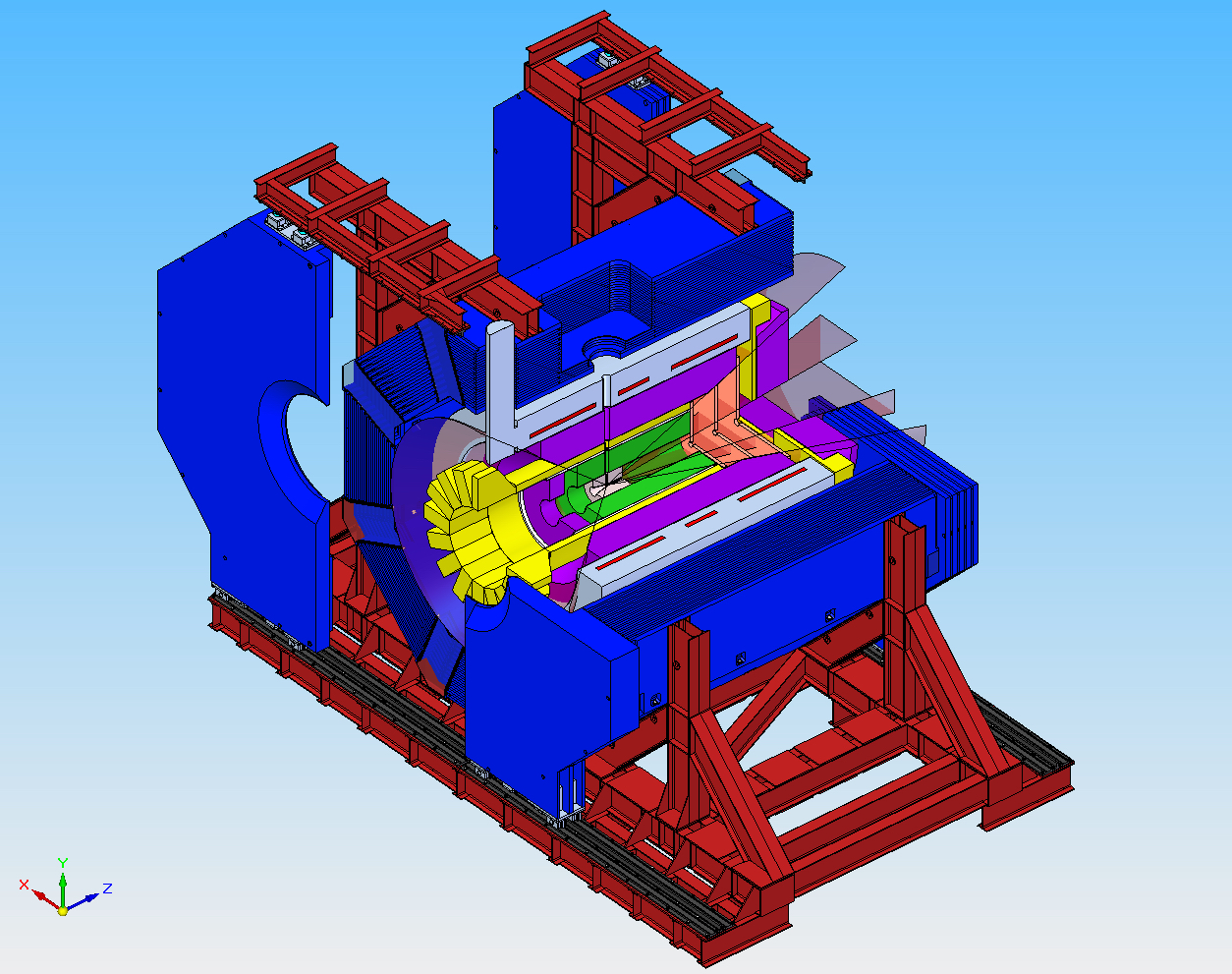
Figure 3.1: View of the Target Spectrometer with the away doors open. For illustration one quarter is cut on this view revealing the cryostat, coil and inner detectors. The antiproton beam would enter from the left along positive $z$. The cones originating at the interaction point indicate the acceptance regions of the different detection systems.

The design was optimised in an iterative procedure taking into account all the detector specific issues, while simultaneously optimising the magnet design in functionality, reliability and cost effectiveness. The design has undergone a dedicated review by independent international experts. This detailed procedure and advice by companies building in the past similar magnets led to the present design. The main features are listed in Table 3.1.

Parameter	Value
SC Material	NbTi
Cable Type	Rutherford
Stabilisation	Pure Al
Operating Current	$\leq 5000\unit{A}$
Current Density	$<60\unit{A/mm^{2}}$
Winding Layers	2
Residual Axial Force	$\leq 30\unit{t}$
Field in Iron	$\leq 2\unit{T}$

Table 3.1: Key features of the solenoid.

Though the magnet design is elaborated from the requirements at it has many similarities with existing and operating magnets at other research institutions. A brief compilation of a few magnets is given in Table 3.2. This shows that it is technically possible to build such a magnet. Moreover, the experience gained in those projects helped in designing the solenoid. Though these solenoids are quite similar, they all lack the special feature of the solenoid that the vertical target pipe is transversing the cold mass of the cryostat at about 2/3 of its length.

	ZEUS	ALEPH	BABAR	BESIII
Location	DESY	CERN	SLAC	IHEP	FAIR
Year completed	1988	1986	1997	2008	2012
Central field (T)	1.8	1.5	1.5	1.0	2.0
Inner bore (m)	1.85	4.96	2.8	2.38	1.9
Cold mass parameters
Length (m)	2.5	7	3.46	3.52	2.7
Energy (MJ)	12.5	137	25	9.5	20
Current (A)	5000	5000	4600	3250	5000
Weight (t)	2.5	60	6.5	4.0	4.5
Cable cross section (mm)	$4.3\times 15$	$3.6\times 35$	$4.9\times 20$	$3.7\times 20$	$3.4\times 25$
Current density ($\unit{\frac{A}{mm^{2}}}$)	78	40	47	41	59
Yoke parameters
Length (m)	15	10.6	6.0	5.8	4.9
Outer radius (m)	4.20	4.68	2.92	$\sim 3$	2.30
Iron layers	10	23	20	9	13
Total weight (t)	1962	2580	580		300

Table 3.2: Comparison of key parameters of some solenoid magnets and the proposed solenoid.

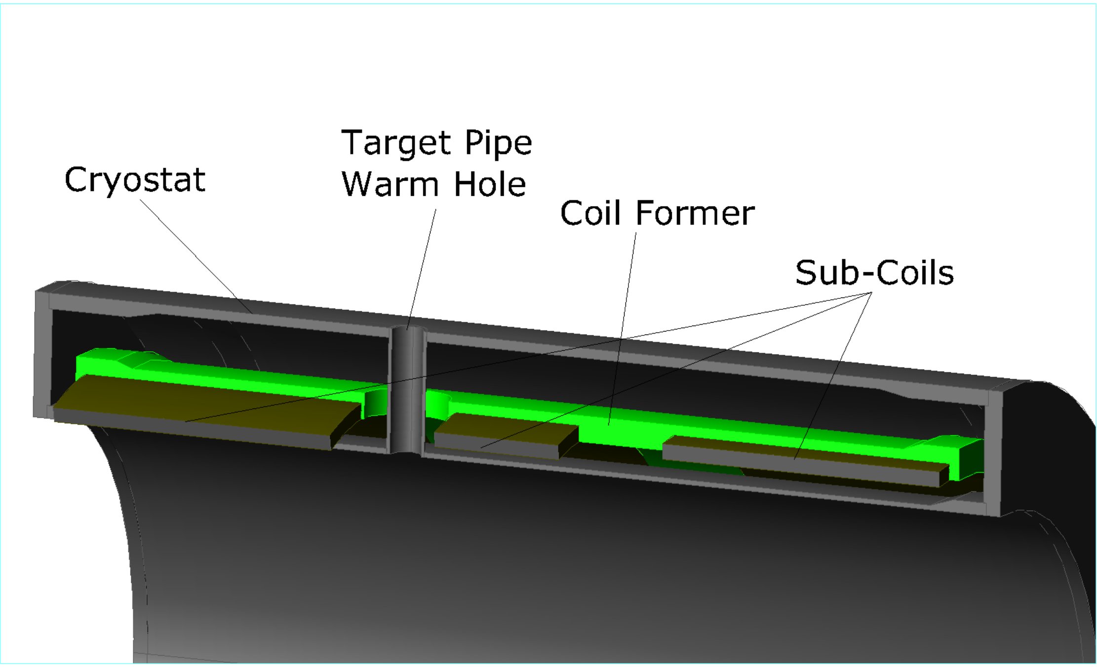
Figure 3.2: Schematic view of part of the coil. The cryostat, coil former and 3 sub coils are shown, while the thermal screens and cooling pipes are omitted.

3.1.2 Cable & Coil Design

The basic feature of the design is the use of a Rutherford-type cable made of NbTi superconductor encased in an aluminum stabiliser that allows for adequate quench protection. A schematic cross section of the coil and cryostat section is shown in Fig. 3.2. A aluminium-stabilised conductor is used which is wound to the inside of the aluminum alloy coil former. The energy to cold mass ratio is $\sim 5.2\unit{kJ/kg}$: this value is similar to many previously built magnets, such as TOPAZ [Yamamoto:1986zd], CDF [Minemura:1985yv], ALEPH [Baze:1987ct], ZEUS [Acerbi:1985yd], H1 [:1986ge], DELPHI [:1983ac]. Since we do not require high transparency for particles, there has been no need to push this ration to even larger values, as it was done for some other magnets (e.g. [Yamamoto:2008zze]). This allows for a design which can safely cope with a residual axial force of 30 t. The coil former cross section is optimised to minimise the stresses on the cable, while allowing the pre-stress of the coil with the coil former end flanges. Cooling will be achieved by liquid helium which runs in pipes welded on the outside of the coil former.

Our concept has benefited from experience gained over the past 25 years with thin superconducting solenoids. The technique was first developed for CELLO [coil:desportes], the first thin solenoid, and has been improved in subsequent designs. Although specifically tailored to meet the requirements of , this design is similar to many operating detector magnets. Table 3.2 shows the main features of some of these solenoids compared to the design.

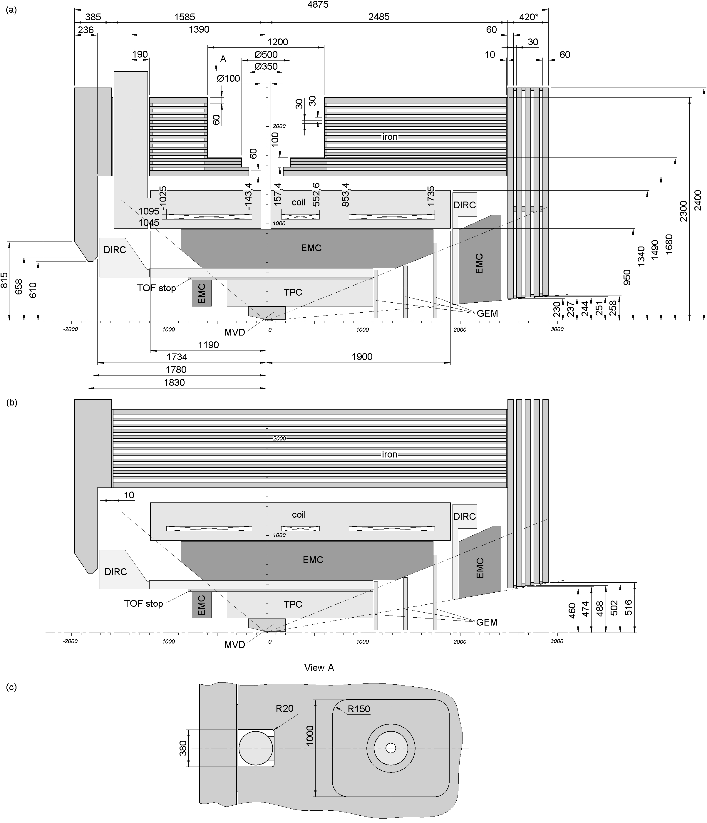
Figure 3.3: Cross sections of the Target Spectrometer showing the yoke layout: a) upper half cross section in the $z-y$ plane showing the recess for the target generator at the top, b) half cross section in the $z-x$ plane c) top view of the upstream top surface showing the cut out for the cryogenic chimney and the target recess. The detectors are indicated schematically for illustration only.

3.1.3 Flux Return Yoke Design

Lamination

A cross section of the planned solenoid is shown in Fig. 3.3. According to the muon range system requirements, the barrel part will consist of 13 steel plates interleaved by 30 mm gaps for allocation of muon detector planes and signal amplifiers. The thickness of the inner and outer steel plates will be 60 mm and of all intermediate plates 30 mm. The downstream end cap will consist of 5 steel plates of 60 mm thickness with 30 mm gaps between plates for accommodation of muon detector panels. The upstream end cap will not be laminated. In order to ensure the unhampered insertion of muon counters, special templates will be used to control the gap thickness between the steel plates during the yoke manufacturing.

End Caps and Passages

The passages for cables and tubes across the yoke are foreseen at the upstream and downstream ends of the yoke barrel. The radial passages and steel spacers between the end caps and the barrel are shown in Fig. 3.4. These spacers are intended to compensate possible gaps between some barrel beams and the end caps. The spacers are designed such that they can be taken out before moving the doors to ensure an undisturbed opening of the doors. Additionally a 1 degree deviation of the door sliding direction from the line perpendicular to the beam axis is foreseen. The gaps for cables will be closed by lids to protect their contents from damage when the doors are moving. The upper beam of the yoke barrel will contain recesses for the target and for the cryostat chimney. The first recess hosts turbo-molecular pumps which are sensitive to magnetic fields, and the latter contains the cooling pipes, current leads and wiring for gauges. The lower barrel beam will have a smaller recess for the target dump.

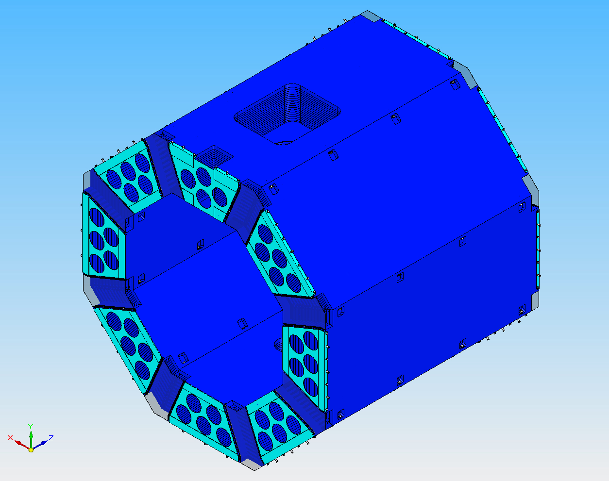
Figure 3.4: Barrel part of the yoke seen from the upstream end. On top the target recess is visible and on the front the face spacers are shown in light blue.

Support Frames

The barrel of the iron yoke is to be surrounded by two outer support frames. Their positions and dimensions are shown in Sec. 3.3. The frames will ease the mounting of the 8 segments of the yoke and ensure the overall rigidity of the yoke, such that both mechanical and magnetic loads result in deformations of the yoke by only a few millimetres (see Sec. 3.3.4). Simultaneously, these frames will take the load of the whole Target Spectrometer and transfer it to the 4 wheel carriages or 6 fixed support points which suspend the movable system on two rails. The doors which can be opened independently will be attached and supported by the same system. An overview is shown in Fig. 3.1 while the details are discussed in Sec. 3.3.

3.1.4 Model for Magnetic Analysis

During the project optimisation, several different Finite Element Model (FEM) codes were used: Ansoft Maxwell [coil:maxwell], ANSYS [coil:ansys] and TOSCA [mag:TOSCA_2003]. A comparison of their results gave us an estimate of the accuracy of the calculations. The iron properties used for computation are those of standard AISI 1010 low carbon steel. We included the material’s non-linear behaviour when saturating. The dependence used for the magnetic induction $B$ on the field $H$ is shown in Fig. 3.5.

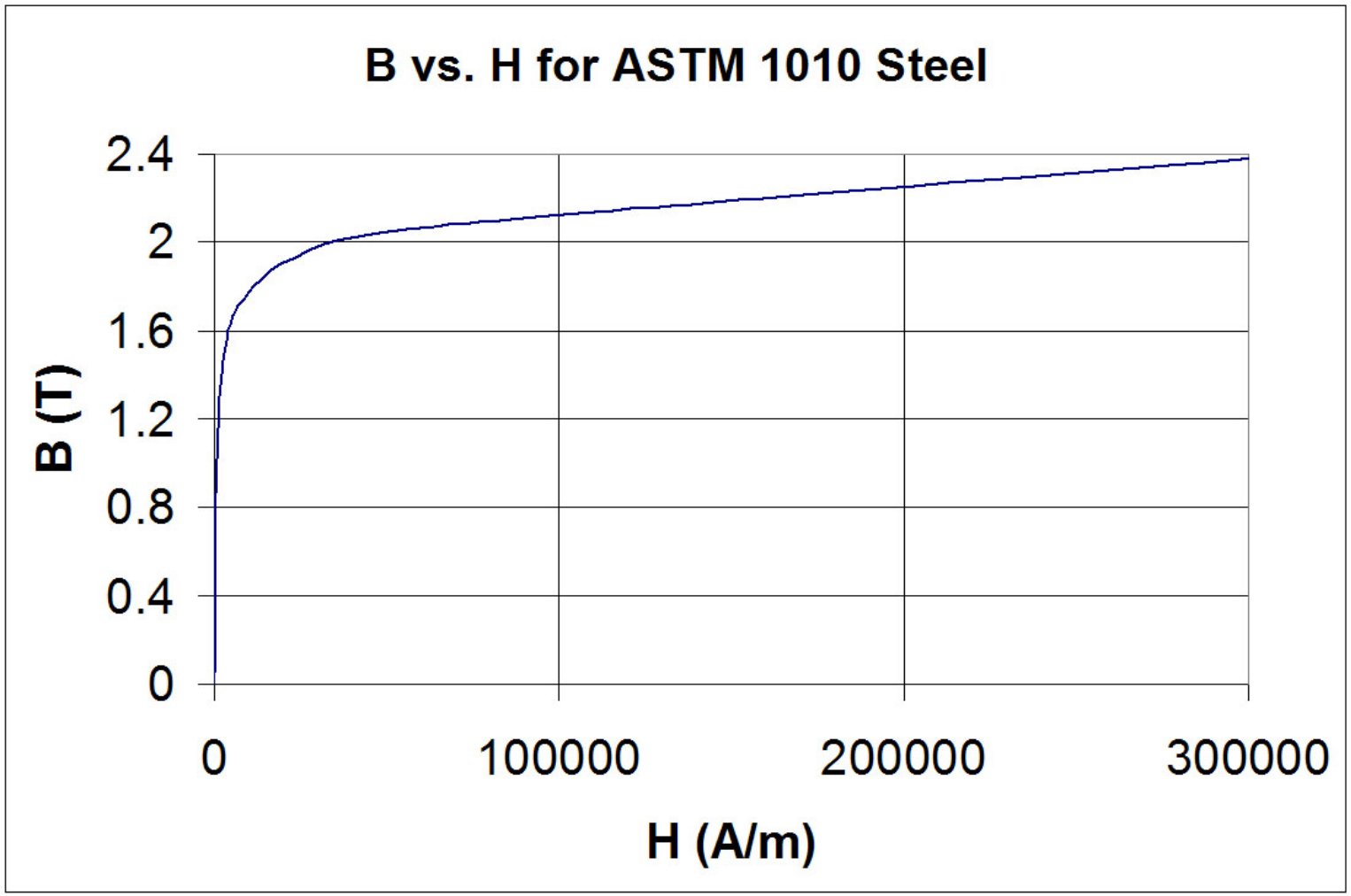
Figure 3.5: Magnetic induction $B$ versus field $H$ for AISI 1010 low carbon steel used for the magnetic calculations.

The magnetic analysis is based on a two–dimensional axially symmetric model and on a complete three–dimensional model. These models include the solenoid, flux return yoke and the doors. The three–dimensional calculations were performed with an accurate 3D model of a quarter of the system and adequate symmetry conditions (see Fig. 3.6).

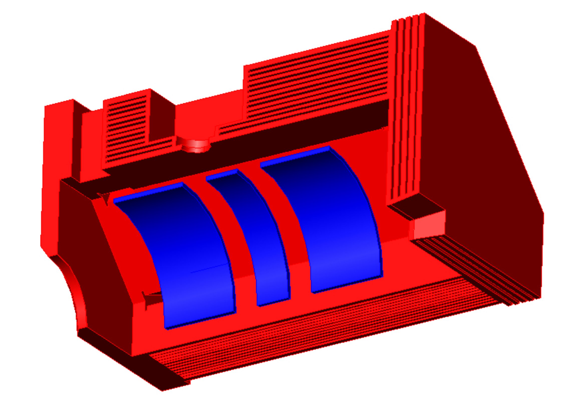
Figure 3.6: Partial model used for the 3D FEM calculations.

All the different calculations gave results which showed deviations smaller than $0.1\%$ in the tracker region. This indicates that we, indeed, can trust the results to such a level of accuracy.

3.1.5 Summary

Following the guidelines from the detector requirements, as laid out in Sec. 2.4, a detailed conceptual design was developed for the solenoid. The main parameters which were achieved during the iterative optimisation procedure are listed in the following.

• Induction field in outer tracker region: $2\unit{T}\pm 1.6\%$.

• Radial field integral $\int{B_{r}(r,z)/B_{z}(r,z)\,dz}$ in the tracker region: $0-2\unit{mm}$.

• Residual axial force on the coil: $20\unit{t}$.

• Design complies with all requirements from the detectors, supplies, space and infrastructure restrictions.

The two following sections detail the proposed design of the coil, cryostat, flux return yoke and support structures. A detailed analysis of the performances of the whole solenoid magnet will be laid out in Sec. 3.4. Sec. 3.5 describes the target and detector integration in the system.

3.2 Coil and Cryostat

A. Bersani

3.2.1 Introduction

The magnet design provides a magnetic field of $2\unit{T}$ with a uniformity of $\pm 1.6\%$ in the tracking region. This will be obtained with a single current density (i.e. a single cable cross section) in three sub-coils connected in series. The coil will be split in three connected sub-coils to leave a gap at the place where the target pipe intersects the magnet. The second sub-coil is needed for symmetry reasons to obtain a good field homogeneity. The central coil will be $395.2\unit{mm}$ in length with 104 turns. Two end coils will be $882.6\unit{mm}$ in length with 232 turns. A better field uniformity may be obtained by reducing the axial length of the two end regions and increasing the current to generate the same field, but this would cause a reduction in stability against thermal disturbance.

For the initial design, the maximum allowed current density in the conductor has been limited to the maximum currently attainable for magnets of this kind, i.e., $80\unit{A/mm^{2}}$ (ZEUS magnet). In these conditions, a cross section of $\sim 80\unit{mm^{2}}$ for the conductor corresponds to a maximum current of $\sim 6400\unit{A}$: our choice of $5000\unit{A}$ will give a good margin for operations. The main parameters of the  solenoid coil are listed in Table 3.3.

Parameter	Value
Central Induction	$2\unit{T}$
Conductor Peak Field	$2.8\unit{T}$
Uniformity in the Tracking Region	$\pm 2\%$
Winding Length	$2.8\unit{m}$
Winding Mean Radius	$1075\unit{mm}$
Amp Turns	$5.68\cdot 10^{6}$
Operating Current	$5000\unit{A}$
Inductance	$1.7\unit{H}$
Stored Energy	$21\unit{MJ}$
Total Length of Conductor	$8000\unit{m}$

Table 3.3: The main parameters of the  solenoid winding.

The coil will be symmetric w.r.t. its centre: the resulting magnetic field will essentially be symmetric inside the cryostat warm bore. The asymmetries in the magnetic field will arise from the asymmetries of the instrumented flux return yoke, which cannot be avoided due to the space requirements from the detectors.

3.2.2 Coil and Cryostat Design

Aluminium Stabilised Conductor

The conductor will be composed of a superconducting Rutherford cable embedded in a very pure aluminium matrix by a co-extrusion process that ensures a good bond between aluminium and superconductor. Table 3.4 shows the main parameters of the conductor.

Parameter	Value
Conductor Type	NbTi
	Pure Al–stabilised
	Co–extruded
Aluminum RRR	$>500$
Conductor Unit Length	$1.6\unit{km}$
Number of Lengths	$5$
Bare dimensions	$3.4\times 24.6\unit{mm^{2}}$
Insulated dimensions	$3.8\times 25\unit{mm^{2}}$
Superconducting Cable	Rutherford type
Dimensions	$8\times 1.15\unit{mm^{2}}$
Strands Diameter	$0.8\unit{mm}$
Number of Strands	$20$
Cu:Sc	$1.5:1$
Filament Diameter	$20\unit{\mu m}$
$I_{c}(B=2.5\unit{T},\,T=4.5\unit{K})$	$>10\unit{kA}$
Insulation Type	Fibreglass Tape
Insulation Thickness	$0.4\unit{mm}$

Table 3.4: Conductor parameters.

The operating current for this conductor will be $50\%$ of the critical current at twice the peak field, giving a large safety margin. In the case of local heating up to $5.2\unit{K}$, there will still be a significant margin on the critical current ($I=0.6I_{c}$). At $2.8\unit{T}$, the conductor critical temperature will be $T_{c}=8.15\unit{K}$, and the current sharing temperature will be $6.3\unit{K}$. This values can be calculated using the following scaling functions, so-called Lubell functions [coil:lubell].

$$T_{c}(B)=9.25\unit{K}\left(1-\frac{B[\unit{T}]}{14.5\unit{T}}\right)^{0.59}$$ (3.1)

describes the critical temperature as a function of the magnetic field on the conductor, and

$$J_{c}(B)=J_{0}\left(1-\frac{T}{T_{c}(B)}\right)$$ (3.2)

describes the critical current density as a function of the magnetic field on the conductor and of the temperature. The working point curves are shown in Fig. 3.7.

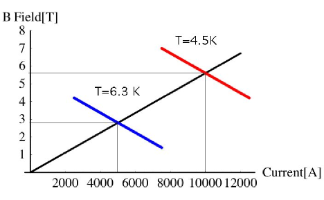
Figure 3.7: Superconducting cable work point calculation. The red line represents the current sharing vs. magnetic field curve at $4.5\unit{K}$ calculated for our cable: the cable was chosen to be critical at twice the current and twice the magnetic field w.r.t. the work ones. The blue line represents the sharing current vs. magnetic field at the work condition ($I=5000\unit{A}$, $B=2.8\unit{T}$): the sharing current temperature is here $6.3\unit{K}$, giving us a safety margin $\Delta T=1.8\unit{K}$.

A simple method to evaluate the stability of the winding consists of considering the enthalpy margin per unit length between the operating and the sharing temperature. This stability parameter will be $\leavevmode\nobreak\ 0.5\unit{J/m}$ for the solenoid, which is identical to the value obtained for the ALEPH and BaBar magnets.

The required superconductor cross section is then calculated to be $4\unit{mm^{2}}$, which means 18 strands are needed, assuming $\alpha=1.2$ and a strand diameter $0.8\unit{mm}$. Together the strands will form a Rutherford cable, 80% compacted, with a cross section of $1.3\times 8\unit{mm^{2}}$

The cross section of the bare cable will then be $3.4\times 24.6\unit{mm^{2}}$. The coil winding can be made using six lengths of conductor, four $1600\unit{m}$ long and two $800\unit{m}$ long, requiring five electrical joints in total. Each joint must have a resistance of less than $5\cdot 10^{-10}\,\Omega$. The length of each joint should be optimised limiting the power dissipation to a few milliwatts. It can be manufactured either by tungsten-inert-gas (TIG) welding (as in the Atlas barrel toroid and CMS), or soft soldering (after electro–deposition of copper).

Electrical Insulation

Electrical insulation is an important aspect of solenoid design and manufacture. Two categories of insulation are required: ground plane insulation between the coil and support cylinder, and turn–to–turn insulation.

• The ground plane insulation must operate at relatively high voltages during quench conditions and will be subjected to strict quality assurance controls. The materials will be fully characterised, electrically and mechanically, before the coil manufacturing, and insulation tests between the cable and the coil former will be performed at $2000\unit{V}$ during the whole winding process. The design of the quench protection systems is based on a maximum voltage to ground of $500\unit{V}$. The ground plane insulation will be made by a $0.8\unit{mm}$ layer of fibreglass fabric inserted between the support cylinder and the solenoid outer layer during the winding. Summing up this insulation layer to the cable insulation we deduce the need for a ground insulation of $\sim 1\unit{mm}$. We are confident from the previous experience on similar solenoids (BaBar, Zeus, CMS) that this ground insulation thickness will be adequate to withstands the quench voltage of $\sim 500\unit{V}$. The insulation will be fully tested at $2\unit{kV}$ along the winding process.

• The conductor will be insulated with a double wrap of $0.125\unit{mm}$ fibreglass tape during winding to give an insulation thickness of $0.2\unit{mm}$ ($80\%$ compacted). The resulting turn–to–turn insulation thickness will be $0.4\unit{mm}$ and will be fully impregnated in the bonding process. Electrical tests will be carried out during winding to detect any failure of insulation. The tests will include regular and continuous testing for turn–to–turn and turn–to–ground insulation.

At the end of the winding process, the fibreglass insulation will be fully vacuum impregnated with high strength epoxy resin. The coil and coil former compound, after the vacuum impregnation, will behave like a monolithic cylinder, making turn–to–turn movements very unlikely.

Winding Support

The winding will be supported by an external aluminum alloy cylinder similar to other existing detector magnets. The winding support is designed for all aspects of force containment, i.e., its weight and the radial and axial magnetic forces. Fig. 3.8 shows these magnetic forces on the solenoid.

The coil former will be built from a single rolled plate of aluminum alloy. The plate will be made of EN-AW 5083 aluminum alloy, heat treated to specification H111 or superior. The CMS experience has demonstrated very good results by a combination of EN-AW 5083, H321 alloy and metal-inert-gas (MIG) welding controlled procedure, being able to avoid stress relieving. Further investigations are under process on this subject.

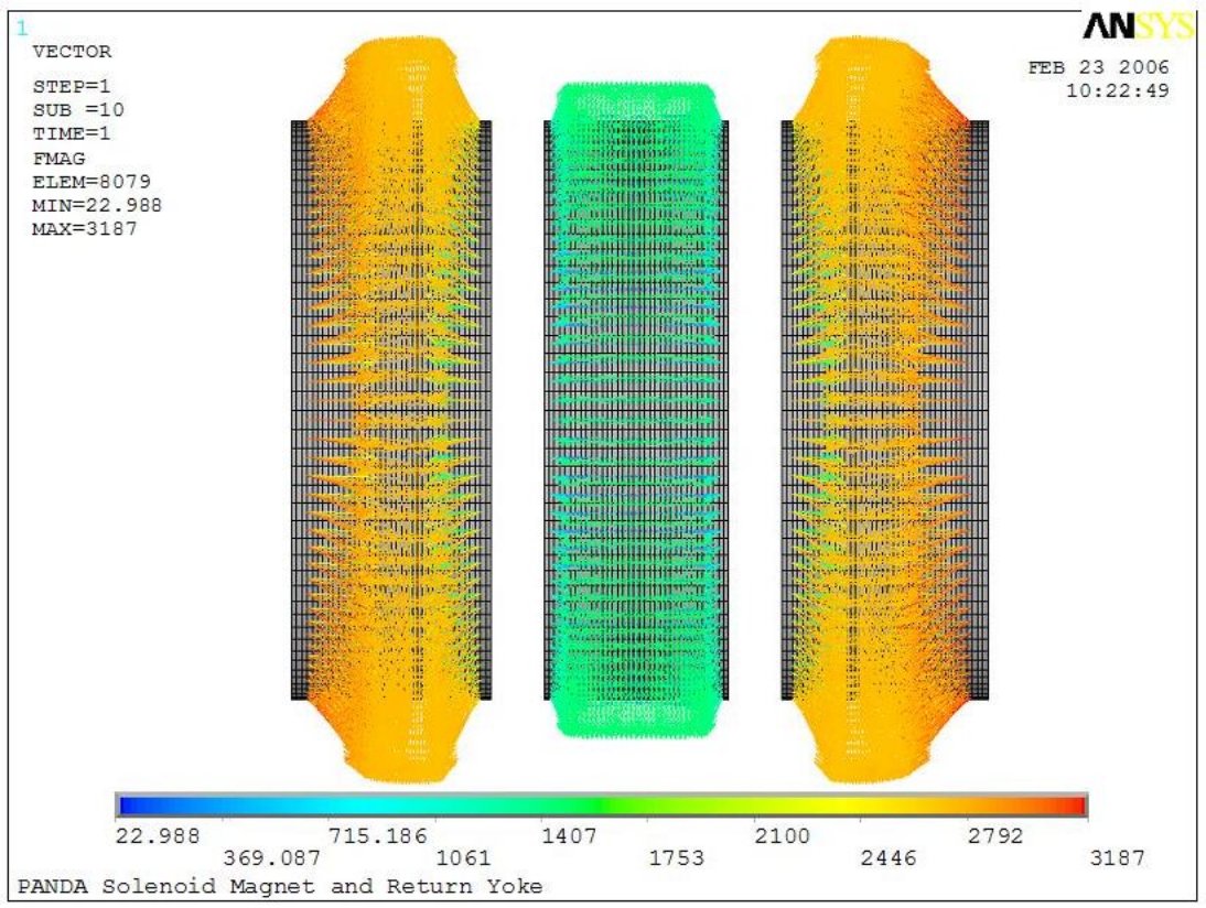
Figure 3.8: The force distribution on the coils (beam direction is left–to–right).

The maximum radial pressure, $\sim 2.90\unit{MPa}$, will be generated in the first and last sub-coils. The aluminum alloy support cylinder surrounds the coiled conductor to counteract these radial pressures and prevent coil movement. An extended stress analysis of the solenoid coil-support cylinder assembly has been developed to investigate the behaviour of the high-ductility pure aluminium stabiliser and epoxy resin under the high radial pressures generated by magnetic forces. The cable was thus simulated including the material non-linear stress-strain curve. As a result, plastic deformations are expected to occur in the coils during the first charge. The amount of these deformations will be small and will ensure that the pure aluminum stabiliser will not be stressed beyond the elastic limit in the subsequent charges. This will help prevent premature quenching during coil energising. Nevertheless, the support cylinder will be capable to contain the deformations of the coils while remaining in the elastic field.

An integrated compressive axial force of $\sim 8\unit{MN}$ will be induced in the winding. According to our calculations, the distribution of the axial force within the coil will be complex. The central part will be slightly axially stressed by a force of less than $1\unit{MN}$. For the calculations of the axial stress inside the winding material we considered the maximum total force we for a sub-coil, i.e., $4.3\unit{MN}$. This would lead to an axial stress of $13\unit{MPa}$ on the pure aluminum, with only the winding supporting the axial forces. However, since the axial force will be transmitted to the outer cylinder, the stress will be considerably lowered. Due to that the shear stress between the winding and outer supporting cylinder will be less than $3\unit{MPa}$. This low value of shear stress will allow the winding and support cylinder to be mechanically coupled through an epoxy impregnation without applying any axial pre-stress to the winding (as it was done for the ZEUS and BaBar magnets). Epoxy impregnation can support a shear stress higher than $30\unit{MPa}$, providing a high safety margin. This will lead to significant simplifications and cost savings in the winding fabrication.

The current design causes axial de-centring forces on the coil due to the iron asymmetry and a residual force of $0.2\unit{MN}$ is applied to the winding. This force will have to be supported by specifically designed and calculated structures. For this purpose, 16 axial bars, made of high-resistance Titanium alloy, have been foreseen, together with 16 radial bars, which account for the weight of the barrel and possible forces due to a misalignment of the assembly with respect to the central axis.

While the preliminary analyses described above decoupled the effects of radial and axial magnetic forces on the coils and support cylinder, a comprehensive 3D FEM analysis has been made simulating the coil and cylinder assembly under the effect of the magnetic field during nominal operations. The results of this calculation (see Fig. 3.9), confirming previous analyses, are pointed out below:

• The radial pressure generated in the windings will cause the pure aluminium stabiliser to exceed its elastic limit, showing permanent deformations after the first charge. Nevertheless, the amount of the plastic deformations will stay negligible and stresses will remain within the elastic range during the subsequent charges.

• The shear stress transmitted through the epoxy resin to the aluminium support cylinder will be fairly low if compared to the resin capabilities.

• The stability of the whole assembly is ensured by the aluminium alloy barrel. The analyses show that the cylinder is capable to contain the radial and axial deformations of the windings without showing permanent deformations.

• Axial and radial supports have also been included in the model. The decentering forces caused by the asymmetry of the return flux and the weight of the assembly will be well supported by the suspension system, the stresses calculated for the bars being well below the elastic limit for titanium alloys (Ti 6Al 4V ELI - grade 23 or Ti 5Al 2.5Sn ELI - grade 6).

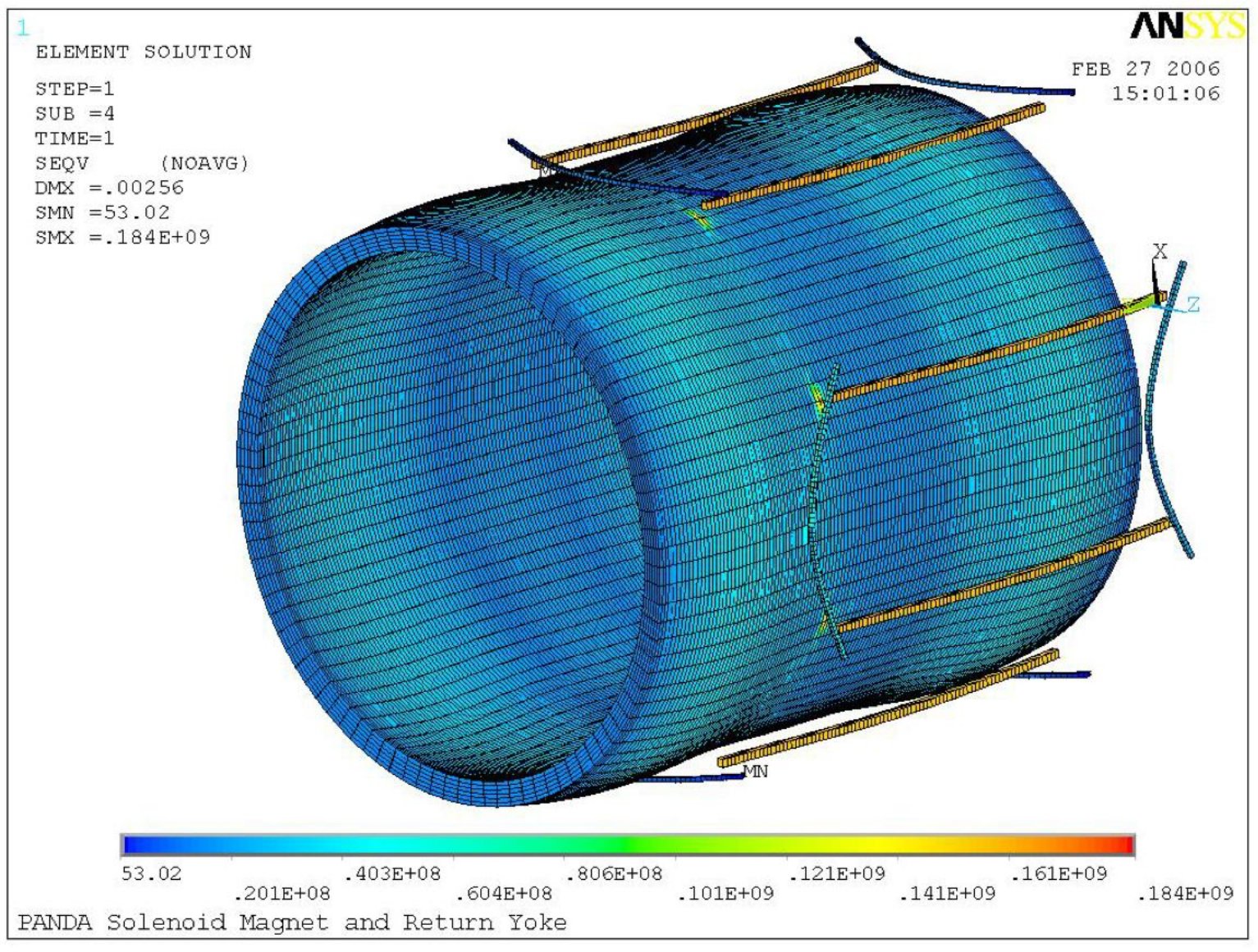
Figure 3.9: Calculated Von Mises stress on the solenoid coil, coil former and supports during nominal operations.

Table 3.5 shows the main features of the cold mass. The values are given at a temperature of $4.2\unit{K}$. The dimensions at room temperature are higher by a factor of approximately $1.004$.

Parameter	Value
Winding:
ID	$2100\unit{mm}$
OD	$2200\unit{mm}$
Length	$2780\unit{mm}$
Weight	$2.2\unit{t}$
Supporting Cylinder:
Material	Al alloy 5083
ID	$2200\unit{mm}$
OD	$2260\unit{mm}$
Length	$2860\unit{mm}$
Weight	$1.8\unit{t}$
Ground Insulation:
Material	Fibreglass epoxy
Thickness	$0.8\unit{mm}$
Total Solenoid Weight:	$4\unit{t}$
Nuclear Interaction Length:
(Assuming Aluminum)
Maximum	$0.2\unit{\lambda_{int}}$
Minimum	$0.15\unit{\lambda_{int}}$

Table 3.5: Cold mass ($4.5\unit{K}$) parameters.

3.2.3 Quench Protection and Stability

Protection Concept

The solenoid will be protected by an external dump resistor which will determine the current decay under quench conditions and allow extraction of $75\%$ of the stored magnetic energy. The quench protection concept is shown in Fig. 3.10, and quench parameters are given in Table 3.6. The protection concept is based on two main criteria.

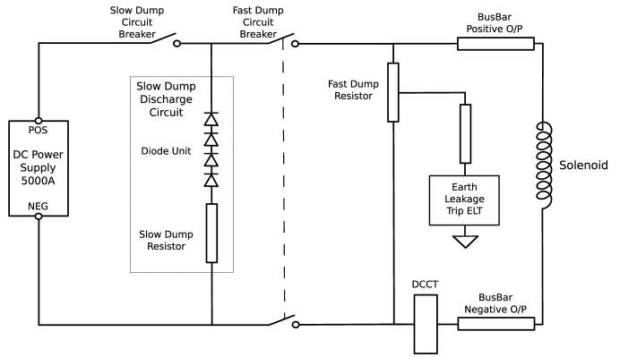
Figure 3.10: Solenoid power and and quench protection concept.

Parameter	Value
Operating Current	$5000\unit{A}$
Stored Energy	$21\unit{MJ}$
Inductance	$1.7\unit{H}$
Quench Voltage	$500\unit{V}$
Protection Resistor	$0.1\unit{\Omega}$
Time Constant	$\sim 17\unit{s}$
Adiabatic Peak Temperature	$100\unit{K}$
Overall Current Density	$53\unit{A/mm^{2}}$
Aluminum Stabiliser RRR	$1000$

Table 3.6: Quench parameters.

Since the calculated stored energy for the magnet is $\sim 21\unit{MJ}$ at an operating current of $5000\unit{A}$, an inductance of $1.7\unit{H}$ is expected. To have a sufficiently fast and effective quench spreading and energy extraction, a $0.1\unit{\Omega}$ resistor was chosen. The time constant of this circuit during a fast discharge will therefore be $17\unit{s}$.

• A voltage limit of $500\unit{V}$ across the solenoid will apply during fast discharge. Centre tapping of the fast dump resistor to ground will limit the voltage to ground to $250\unit{V}$. The centre–tapped resistor will also allow the measurement of ground leakage currents as a safety and diagnostic tool.

• An upper temperature limit of $100\unit{K}$ will apply during quench conditions. This limit will give very good safety margins against the peak temperature and thermally induced stresses at quench.

During a quench, it is foreseen that a large fraction of the liquid helium present in the cooling circuit will boil off. The circuit is dimensioned to face a possible failure of the supply system, which will make the pressure in the pipes as high as at the outlet of the liquefier, i.e. $20\unit{bar}$. If the pressure should get higher, a proper system of safety valves will open to avoid damages.

The quench detection-protection circuit shown in Fig. 3.10 will act also as emergency discharge system, to be used any time a fast shutdown of the solenoid would be needed and we would like to avoid an excessive heating of the cold mass, which can lead to a quench of the winding. This rapid discharge will be used to protect the solenoid (or other sub-detectors) against failure of any external infrastructure, such as power supply, main power and refrigeration failures.

When a failure in the infrastructure operation was detected, the “slow dump breaker” (shown in Fig. 3.10) would open, and the magnet current would be dumped by the slow dump resistor through the diode unit. The value of this resistor is chosen to prevent the transition of the superconducting coil produced by the power dissipated by the magnetic flux variation and the eddy currents in the coil former. Simulations of the transient behaviour of the winding showed that a discharge time constant of $600\unit{s}$ will prevent any unwanted heating effect. Given the solenoid inductance of $1.7\unit{H}$, the discharge time is fixed by the value of the slow dump resistor: in our set-up, the resistor value is $3\unit{m\Ohm}$, rated for a peak power dissipation of $15\unit{kW}$.

Quench Analysis

A preliminary quench analysis of the  solenoid has been made using a code developed for indirectly cooled solenoid design. The code models the thermal and inductive behaviour of the solenoid in order to account for quench–back effects and heat transfer to the support cylinder. This analysis shows that quench–back is predicted about two seconds after opening the protection circuit breakers.

Several different calculations were performed (courtesy AS-G Superconductors, formerly known as Ansaldo superconductors), simulating a local temperature rise in different locations on the coil. It was seen that the worst situation would be encountered when the quench was generated in the downstream, internal coil. The simulated temperatures of the various windings are plotted in Fig. 3.11. In no scenario the temperature on the superconducting cable exceeded $65\unit{K}$, and in every situation the temperature, after a short period, will drop to $\sim 40\unit{K}$.

Figure 3.11: Temperature evolution in the coil after a quench, as a function of time. The coil was divided into 6 sectors, the 3 sub-coils divided into the 2 layers. The calculation refers to the worst scenario, i.e. the quench is generated in the downstream sub-coil, internal layer, labelled as number 4. The coil sectors are numbered this way: 1. external upstream; 2. external central; 3. external downstream; 4. internal downstream; 5. internal central; 6. internal upstream (courtesy AS-G Superconductors).

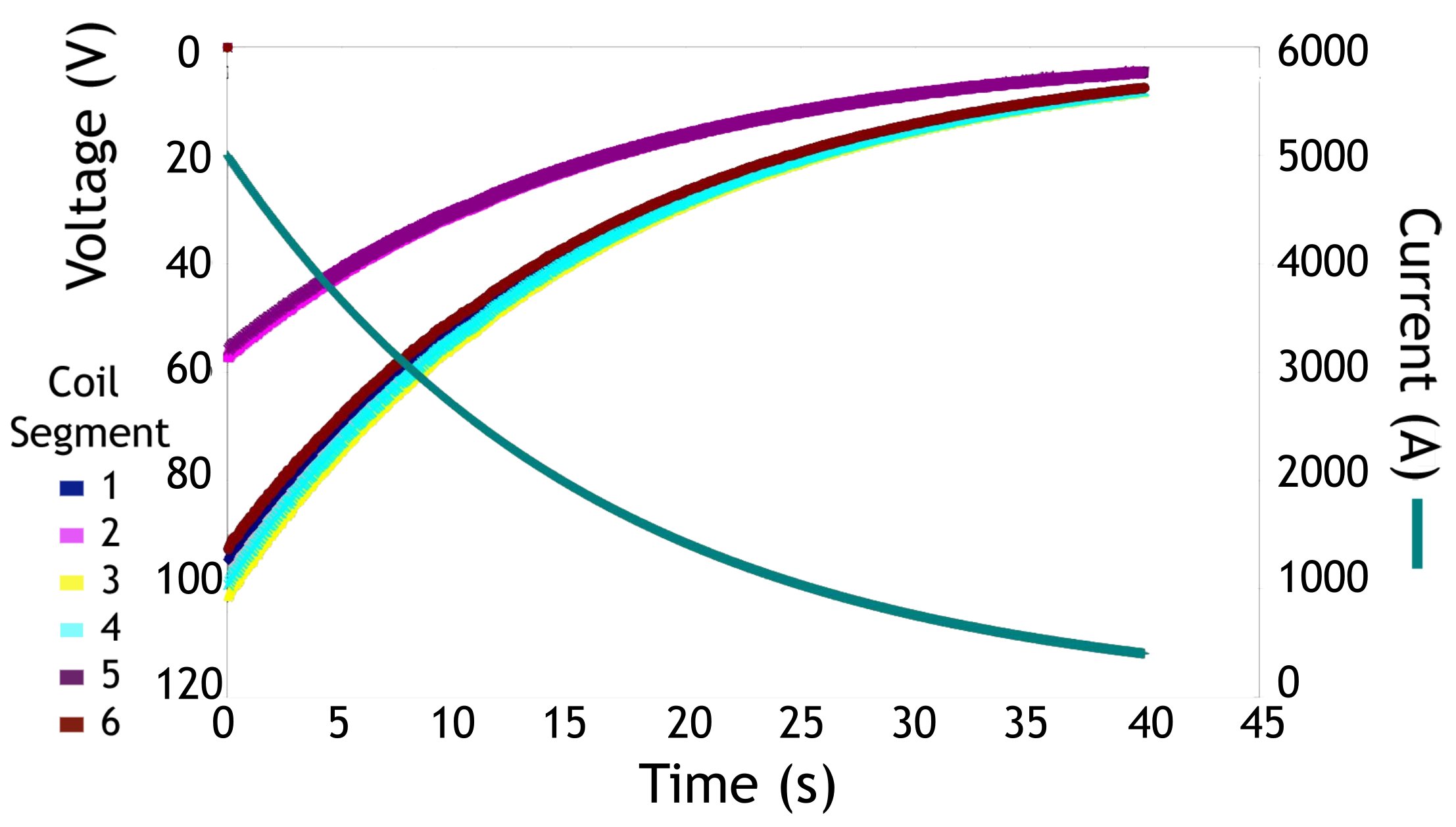
Figure 3.12: Voltage and current evolution in the coil after a quench as a function of time. The coil was divided into 6 sectors, the 3 sub-coils divided into the 2 layers. The calculation refers to the same scenario as 3.11 (courtesy AS-G Superconductors).

The role of the coil former as a quench spreader has been studied comparing the temperature rise with and without the coil former itself: this case is similar to the one of a coil former made of a poor heat and current conductor, such as stainless steel, carbon fibre or similar. Even in this configuration, the quench would remain limited to the coil in which it started and in the neighbouring one, and the temperature would never exceed $80\unit{K}$.

Fig. 3.12 shows the voltage at the ends of each winding and the current in the coil after a quench: a time constant of $\sim 17\unit{s}$ is obtained, confirming the value of inductance of $\sim 1.7\unit{H}$ obtained from pure magnetic calculations.

Stability

The solenoid coil will be indirectly cooled using the technology established for existing detector magnets such as DELPHI and ALEPH. Reliable operation of those magnets has demonstrated that safe stability margins can be achieved using high–purity, aluminum–clad superconductors in a fully bonded, indirectly cooled coil structure.

The conductor stability has been estimated using an analysis code in order to establish the minimum quench energy (MQE) for transient heat pulses. The computed minimum quench energy is $1.4\unit{J}$. The computed minimum quench length (MQZ) is $0.6\unit{m}$. These margins are considered to be safe for the solenoid due to its low–stress design.

3.2.4 Cold Mass Cooling

Cooldown

The cold mass cool down will be accomplished by circulating cold helium gas either directly from the refrigerator or from a storage Dewar with gas mixing.

Operating Conditions

.

Under operating conditions, the cold mass will be cooled by circulating two–phase helium in pipelines welded on the coil support cylinder. The cooling circuit will be driven either by forced or natural (thermo–syphon) convection. This technology is established and yields the simplest operational mode. The thermo–syphon cooling circuit is designed for high flow rates to ensure the correct quality factor for the helium. The circuit will be fed through a manifold at the bottom of the support cylinder. The cooling circuits will be welded to the support cylinder surface with a spacing of $\sim 0.3\unit{m}$ to limit the temperature rise. The cooling pipes will terminate in an upper manifold. The circuit will be designed to provide operation during quench conditions. In order to confirm these assumptions, a finite element model of 1/8 (thanks to the axial symmetry) of the coil–barrel has been developed. The maximum temperature rise will be equal to $0.31\unit{K}$ compared to the design temperature of $4.5\unit{K}$ (see Fig. 3.13). This assumes the estimated static heat loads (reported in the next paragraph), a pipe diameter equal to $20\unit{mm}$ and a liquid helium mass flow of $28\unit{g/s}$. The conceptual layout of the cold mass cooling circuit (natural convection solution) is shown in Fig. 3.14.

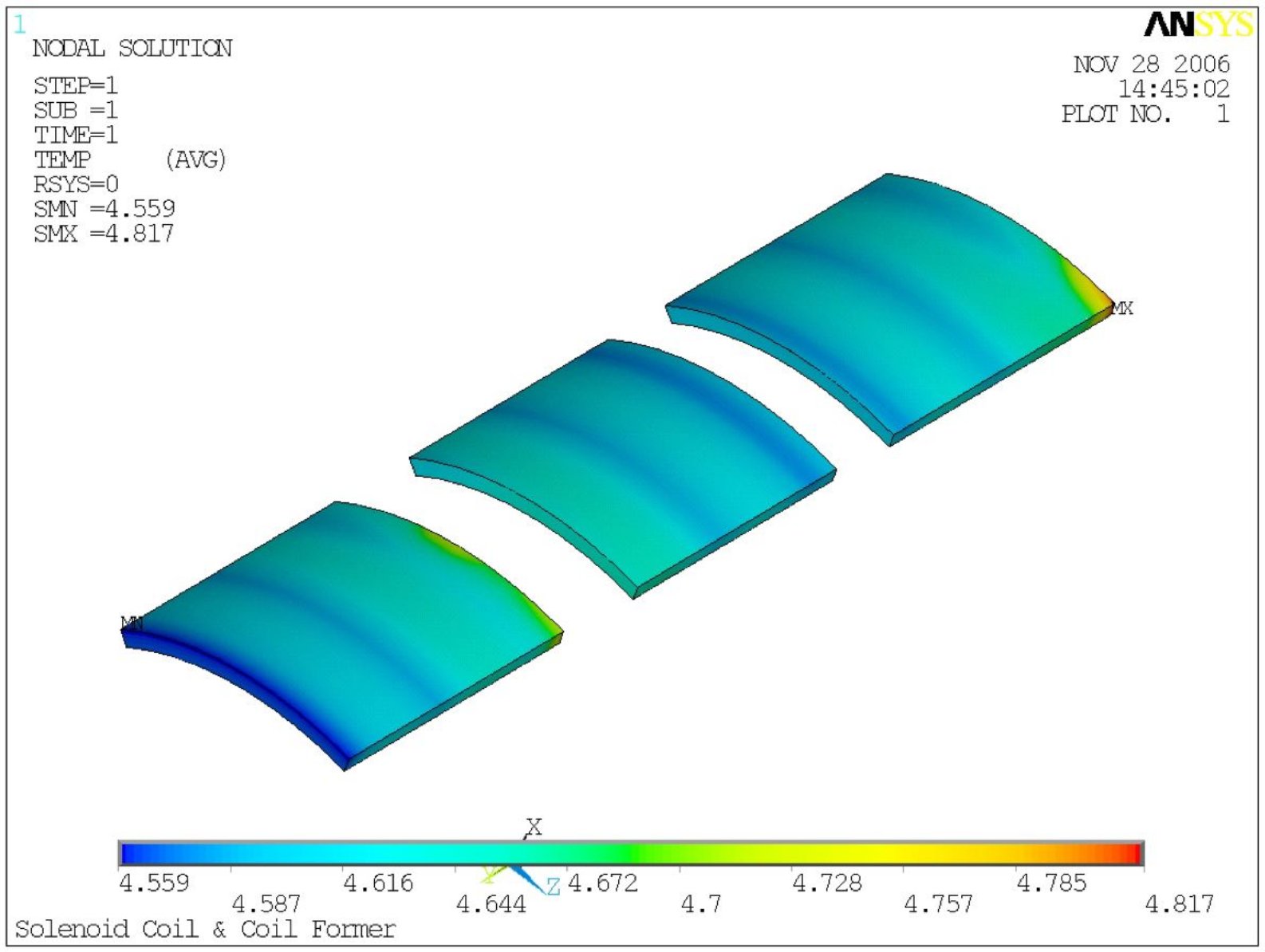
Figure 3.13: Temperature distribution in the coil during normal operation. The calculation was performed on a section of the assembly taking into account the coil former assembly, all the heat leaks and the symmetry of the system.

Figure 3.14: Cold mass cooling circuit. The cryogenic supply chimney passes through a cut–out in the barrel flux return (shown top left).

Heat Loads

The estimated static heat loads for the solenoid are given in Table 3.8. Eddy current heating in the support cylinder will cause additional heat loads during charging of the solenoid. However, for a solenoid charging time of $30\unit{min}$, the estimated transient power will be $8\unit{W}$, which is small compared to static heat loads.

3.2.5 Cryostat Design

Vacuum Vessel

The cryostat consists of an annular vacuum vessel equipped with radiation shields and super-insulation. The vacuum vessel is designed to satisfy a number of basic criteria listed in the following.

1. To support vacuum loads in accordance with recognised pressure vessel codes.

2. To carry the cold mass and radiation shield weight through the insulating supports.

3. To support magnetic loads (20 metric tons of axial forces with a safety factor of 4, as foreseen for suspended loads) during nominal operations.

4. To operate with deflections of less than 1 mm under all loads when mounted in the flux return barrel.

5. To carry the weight of the inner detectors. (The Barrel EMC weight is already 20 metric tons.) The calculation has been made assuming a total weight attached to the cryostat of 50 metric tons.

The vacuum vessel is designed as two concentric cylinders with thick annular end plates, all of aluminum alloy 5083; its basic parameters are given in Table 3.7. A cross section of the downstream end is shown in Fig. 3.15. The minimum thickness of the different parts composing the cryostat has been designed, will be fabricated and will be inspected according to the intent of the EC Euronorm codes for Unfired Pressure Vessels, EN 13445 [EuroCode13445], but will not be code-stamped. For steel structures, the allowable design stresses follow the standard guidelines of European standards [EuroCode3]. Bolted connections and fasteners will conform to their recommended torques and allowable stresses depending on the connection.

Envelope Dimensions
Inner Radius	$950\unit{mm}$
Outer Radius	$1340\unit{mm}$
Length	$3200\unit{mm}$
Inner Cylinder Thickness	$10\unit{mm}$
Outer Cylinder Thickness	$30\unit{mm}$
End Plates Thickness	$50\unit{mm}$
Materials	AL5083, AISI 304
Design Loads
Vessel Weight	$6\unit{t}$
Cold Mass	$4\unit{t}$
Calorimeter	$18\unit{t}$
Other Detectors	$3\unit{t}$

Table 3.7: Vacuum vessel parameters.

Figure 3.15: Cross section of the vacuum vessel detailing the downstream end where the rods which suspend the cold mass inside the vessel are attached. These take the axial load during operation.

A preliminary finite element structural analysis of the vessel has confirmed that design criteria (1)$\div$(4) can be met with reasonable safety factors. In our model maximum vessel deflections are less than $1\unit{mm}$, and stress levels peak up to $70\unit{MPa}$ with all loads applied (see Fig. 3.16). The cryostat could also be made of AISI 304 Stainless Steel; in this case, a increased stiffness and increased stress levels are expected.

Figure 3.16: Cryostat FEM model, equivalent stress with all loads applied.

Thermal Shielding

The cryostat will be equipped with radiation shields, which will operate at 40–80 K, and super-insulation. The shields are cooled by helium gas supplied directly from the refrigerator. About 30 layers of super-insulation separate the vacuum vessel walls from the radiation shields. Another five layers will be installed between the shields.

Services

Cryogenic supplies and current supplies will be connected from a service turret to the cryostat through the service chimney in a suitable slit at the backward end of the yoke barrel. Current leads and local control valves will be mounted in the services turret.

We foresee to use standard copper counter-flow cryogenic current leads rated to the running current of the magnet: this corresponds to a liquid helium consumption of $17\unit{l/h}$. Cryogenic relief valves will also be mounted in the service turret for quench and refrigeration failure conditions.

3.2.6 Coil Assembly and Transport

The coil will be assembled inside the cryostat at the manufacturer’s plant. Electrical and cryogenic connections will be made inside the chimney so that the coil can be tested before shipping.

A complete cooldown will be carried out from room temperature to the operating temperature of $4.5\unit{K}$. The cooldown will allow checking of cooling time, temperature control, heat loads, and full operation of sensors. A magnetic test will also be performed at low field ($30\%$ of the operating current) to check superconductor operation, the joint resistance, and the additional losses due to the eddy currents in the outer structural cylinder at the coil ramp-up.

Before delivering the magnet, but after the tests at the factory, the end flanges will be dismounted to allow a hard connection of the cold mass to the cryostat walls. Depending on the transport facilities, the cryogenic chimney may also be dismounted. In this case, the electrical and cryogenic connections also must be dismounted and protected against breakage.

The setup of the yoke, cryostat and solenoid is compulsory for the installation of all the detectors of the Target Spectrometer. This is due to the fact that the cryostat itself provides mechanical support for the various detectors. Therefore, before the detector assembly, tests and commissioning of the magnet have to be completed.

3.2.7 Cryogenic Supply System and Instrumentation

The operation of the superconducting solenoid requires both liquid helium (4.5 K) and cold helium gas ($20\unit{K}-100\unit{K}$) for cooldown and refrigeration of the thermal shields. Similar systems have been used successfully throughout the HEP community. A summary of the cryogenic loads is given in Table 3.8.

Magnet Heat Loads at 4.2K
Item Parameter	Load
Cold Mass	$4000\unit{kg}$
Total Surface Area	$44\unit{m^{2}}$
Radiation Heat Flux (Design)	$0.07\unit{W/m^{2}}$
Radiation Heat Load (Design)	$3.1\unit{W}$
Conduction Heat Load	$2.2\unit{W}$
Cable Joints	max $2\unit{W}$
Cryogenic Chimney	$10\unit{W}$
Gas Load	$1\unit{W}$
Eddy Currents ($1500\unit{s}$ ramp time)	$10\unit{W}$
Total $4.5\unit{K}$ (SF of $2$)	$57\unit{W}$
Magnet Shield Heat Loads at 60K
Item Parameter	Load
Shield Mass	$1000\unit{kg}$
Total Surface Area	$44\unit{m^{2}}$
Radiation Heat Flux (Design)	$1.3\unit{W/m^{2}}$
Radiation Heat Load (Design)	$57\unit{W}$
Conduction Through Supports	$17\unit{W}$
Conduction To Shields	$150\unit{W}$
Diagnostic Wires	$1\unit{W}$
Gas Load	$2\unit{W}$
Eddy Currents ($1500\unit{s}$ ramp time)	$10\unit{W}$
Total $60\unit{K}$	$237\unit{W}$

Table 3.8: Cryogenic heat loads.

The solenoid will be equipped with a full set of instrumentation sensors for monitoring, control, and diagnostic purposes. Instrumentation includes temperature sensors for the cold mass, shield cryogenic flow monitoring, and strain gauges in the coil support cylinder. Voltage taps will monitor the electrical resistance of the conductor joints and will provide quench detection. The quench detection systems will be hardwired to interlocks. The solenoid instrumentation and controls will be integrated with the experiment and refrigeration controls.

Figure 3.17: Proximity cryogenics scheme.

The fully automatic liquid helium plant will be equipped with a process control system and all required logic and software necessary for all operational modes. Control and monitoring of the cryogenic plant and the magnet coil, together with remote control and monitoring of the compressor room, will be carried out from a control room adjacent to the plant room. Main operating parameters will be delivered to the data acquisition and monitoring systems. A scheme of the proximity cryogenics is shown in Fig. 3.17.

3.2.8 Cryostat and Cryogenic System Safety

Vacuum System Safety

The cryostat and cryogenic turret of the solenoid, as reported in Section 3.2.5, will be built according to the EC specifications for the Boiler and Pressure-Vessel Code [EuroCode13445]. The worst case scenario concerning the safety of the cryostat would arise, if a leak evolved in the part of the liquid helium (LHe) cooling circuit that runs through the vacuum vessel. Only in this case the pressures balance could actually be reversed, and the pressure inside the cryostat could exceed the atmospheric pressure.

The cryostat vacuum vessel, turret and all connections was verified to be resistant resist up to a pressure of $150\unit{kPa}$ from the inside. This provides a good safety margin, as the the coolant circuit will be working at an absolute pressure of $125\unit{kPa}$ and we foresee safety valves (see below). For the outer shell the stability against a pressure reverse is easily guaranteed, since it is designed to work with $100\unit{kPa}$ from the outside. This is naturally different for the inner wall of the cryostat, which is designed to keep, under normal operation, the atmospheric pressure from inside. However, the inner wall of the cryostat is designed to keep safely the full load of the detector, mainly the weight of the EMC with a minimum deformation. The extra thickness needed to fulfil this requirement is more than enough to guarantee the cryostat against buckling of the inner wall in case of a pressure reversal due to a leak in the helium circuit.

A system of safety valves has been foreseen to prevent an excessive pressure rise in the cryostat vessel and chimney. A relief valve opening at $130\unit{kPa}$ (absolute pressure) is foreseen. This corresponds to an over-pressure of $30\unit{kPa}$ relative to atmospheric pressure to which the vessel is subject from the outside. In case of LHe vaporisation the relief valve would open, venting the helium gas to the atmosphere preventing damages to the cryostat vessel. As a redundant safety measure, a burst disk opening at $150\unit{kPa}$ is foreseen to cover the unlikely event that the relief valve malfunctions.

Proximity Cryogenics Safety

The choice of indirect cooling of the solenoid will greatly reduce the amount of liquid helium in the cryogenic system. The pipes, guaranteeing the coil refrigeration, will contain $\sim 60\unit{l}$ of refrigerant. This includes the two manifold placed on the top and on the bottom of the winding for the thermo syphon circulation. Another $\sim 50\unit{l}$ of liquid helium will be stored in the current leads bath housed in the reservoir contained in the cryogenic turret of the cryostat.

The operating pressure of the coil cryogenic system will be $125\unit{kPa}$, corresponding to a coolant temperature of $4.5\unit{K}$. The two phases liquid helium used by the cooling system will be fed to the control Dewar trough a transfer line from a $4000\unit{l}$ buffer-storage Dewar, connected to the helium liquefier during normal operation. This buffer tank will give the coil cryogenic system the capability to operate for more than a day in case of refrigerator shutdown. The buffer storage will decouple also the refrigerator from the solenoid cryogenics in case of refrigerator failure.

In the worst case, the gas would be transferred into the buffer-storage at the full pressure of the run compressor of the liquefier ($20\unit{bar}$) rather than into the cooling circuit of the solenoid. In this case it would be vented to the air trough the relief valve or burst disks. Furthermore, it will help that the buffer-storage and the control Dewar will be connected trough a long liquid helium transfer line. This line will hydraulically decouple the two reservoirs in the scenario of a liquefier failure with the $20\unit{bar}$ helium gas at the temperature of the last heat exchanger ($\sim 20\unit{K}$) transferred into the system.

As an additional safety measure, we decided to design all the cooling loops and distribution lines inside the cryostat (including the intermediate radiation shields) for a nominal operating pressure of $20\unit{bar}$.

The control Dewar in the cryo-chimney, operating at $125\unit{kPa}$, is designed for a pressure of $600\unit{kPa}$ (6 absolute bar) and will be equipped with a relief valve venting the vessel to the atmosphere for an overpressure $\Delta p=50\unit{kPa}$ ($p=1.5$ bar) in case of helium boiling off due to a quench or vacuum failure. A burst disc opening at $600\unit{kPa}$ protects the inner vessel of the control Dewar in the extreme case of a total malfunction of the relief valves.

Seismic Safety Considerations

The coil and cryostat of the solenoid are designed to safely keep in operation static forces exceeding ten times the weight of the object. For this reason, from a static point of view, these objects are safe for earthquakes not exceeding magnitude of 3, corresponding to the strongest event registered in the Darmstadt surroundings in the last decades.

A static analysis gives only part on the information needed to guarantee the seismic safety of a complex and composite device as the detector. To ascertain the seismic safety of the system, a transient analysis of the system using an excitation force reproducing the frequency spectra of the Darmstadt seismic activity is needed. The results of seismic analyses are strongly dependent from the component geometry, mechanical features and suspensions. They will be performed as the most important check once the detector layout fully defined and the different options on the sub detector choice and mounting procedure are well defined and frozen.

3.3 Instrumented Flux Return

Y. Lobanov

3.3.1 Introduction

The main purpose of the iron yoke of the Target Spectrometer will be to serve as flux return for the magnetic flux produced by the superconducting solenoid. The details of design of the return yoke will contribute significantly to the shape and the value of the field in the central region, where it is needed for momentum determination. The effect on the absolute value of the magnetic induction field is due to the strong reduction of the reluctance of the magnetic circuit, that enhances the field strength, allowing for a smaller coil at equal fields. In the region of the central tracker the contribution of the yoke to the total magnetic field will be about 12%.

With a properly studied shape, in addition, it is possible to adjust the field flux lines orientation, reducing the radial components of the field itself. Only with a dedicated and optimised design of the flux return yoke, in close interplay with the coil design, the challenging requirements concerning the radial field component in the central region (see Sec. 2.4.3) can be reached.

Furthermore, the presence of this great amount of iron provides the shielding of the outside area from the strong fields produced by the coil. In this region magnetic fields are unwanted and there are strict requirements for the maximum allowable stray fields, ranging 3 orders below the required field in the central region.

The flux return yoke must serve as range system for the identification of muons, too. A system of interleaved detectors and absorbing material is ideally suited for the detection of muons and their discrimination versus pions. Thus, the whole barrel and downstream door will be fully laminated, to allow maximal instrumentation for muon detection. Besides that, the yoke will provide a solid frame for mounting the cryostat and the detectors.

The yoke will consist of a barrel part, with octagonal shape, which will be laminated in 13 layers. A hole of 350 mm in diameter through the barrel part of the yoke is foreseen to accommodate the internal target system, and another one to host the cryostat chimney. Both ends will be closed with end doors. The downstream door will be laminated in 5 layers, while the upstream door does not require lamination. The upstream door will have a central round hole while the downstream door will feature a rectangular one which opens $5^{\circ}$ and $10^{\circ}$ in the vertical and horizontal planes, respectively. Both end doors will be separated into two halves. The end doors will be sliding on skids. Thus they can be opened independently to allow access for maintenance of the inner detector systems.

At both ends of the barrel part, in the octagon corners, proper slits are foreseen, to allow the routing of cables and services for the detector hosted inside the yoke itself.

The Target Spectrometer, hence the instrumented flux return and everything attached to it, will be mounted as a whole on a movable rail-guided carriage to be transported from the assembly area to its operation position. An overview of the full Target Spectrometer from the downstream side is shown in Fig. 3.18.

Figure 3.18: View of the Target Spectrometer from downstream showing the yoke design and the opening doors.

Figure 3.19: Cross-section of the flux return yoke and the support structure in the $z-y$ plane. The beam would come in from the left and interact with the target at the line crossing in the middle of the drawing. The recesses for the target and the cut out for the cryogenic chimney are clearly visible. The view shows the door opening mechanism to the left and right and the carriage on a rail system at the bottom.

3.3.2 Structural Design

The flux return yoke will be divided in a barrel part and end caps on each end which will be realised in two halves each, such that they can be opened as sliding doors. The barrel octagon with its support frame will form an independent self supporting unit which also carries the weight of the cryostat and all the nested detectors. During operations, all parts of the yoke, including the doors, will be rigidly fixed to each other to provide the best mechanical stability.

Barrel Part

In our design the barrel in realised by joining eight beams of 4.05 m length and a trapezoidal shape in an octagon with an outer diameter of 4.6 m. The structural strength will be obtained with an external support structure, consisting of two rings surrounding the barrel on both ends. Two lower beams under the rings and several perpendicular beams will form a carriage, which suspends the whole system. The cross section of the iron yoke is shown in Fig. 3.19.

The beams will be constructed as stack of plates which will be welded using spacers of 30 mm height at both longitudinal edges (i.e. along the $z$ axis). This will ensure that the beams can be equipped with detectors in all their section, except a small area around the corners. As all connections will be realised along the edge of the beams, the installation and service of the detectors can be done independently of the mounting of the yoke. Please refer to Fig. 3.20 for details. Each beam will be fixed to the adjacent beam by means of eight bolts at every butt of the inner and outer plates (Fig. 3.20). Additionally, interlock connections will be used at the barrel beam interfaces.

Figure 3.20: Cross-section and 2 details of one beam of the octagonal barrel. View A shows a top view of the recess for the mounting of the beam to the adjacent neighbour. View B details the connection of the plates.

According to the requirements on the minimum dimensions of the cables and pipes crossing the barrel part of the flux return (see Table 2.7), proper recesses in the barrel are foreseen. These recesses will be provided at the corners of the octagon, both at the upstream and downstream ends of the barrel. The size of each recess will be $140\times 420\unit{mm^{2}}$. The shape and positions of the recesses were chosen taking into account the required space for cables and pipes, the maximum mechanical stability of the flux return and the minimisation of space inside the yoke that could not be occupied by muon counters. At the same time, the influence of the recesses on the magnetic field in the central tracker region will be insignificant, as shown in Sec. 3.4. The recesses will be closed by lids to protect their contents from during doors closing and opening. The layout of the upstream part of the yoke barrel with the cut-outs for cables and pipes is shown in Fig. 3.21

Figure 3.21: Upstream part of the yoke barrel showing the cut-outs for cables and pipes

Layer	Thickness	$r_{min.}$	$r_{max.}$
	/ mm	/ mm	/ mm
1	60	1490	1550
2	30	1580	1610
3	30	1640	1670
4	30	1700	1730
5	30	1760	1790
6	30	1820	1850
7	30	1880	1910
8	30	1940	1970
9	30	2000	2030
10	30	2060	2090
11	30	2120	2150
12	30	2180	2210
13	60	2240	2300
TOTAL	450 (iron)	1490	2300

Table 3.9: Table detailing the radial iron lamination of the solenoid yoke. All dimensions are given in the radial direction, normal to the octagonal face of the yoke, beginning from the innermost layer to the outermost. The layers are counted accordingly outward from the centre.

Figure 3.22: Downstream end cap of the flux return yoke. A view in the $x-y$ plane is shown in the upper panel, while the lower panel shows a top view of the doors and the mounting rods. The rails for the door movement are omitted in this figure for better visibility.

Upstream and Downstream End Doors

The upstream end cap will consist of 13 steel plates of 30 mm thickness consolidated in a package by means of welding trough holes under pressure. The beam consolidation of the solid yoke of the ALICE magnet has been done in the same way. It will be constructed in two parts and can be opened to the sides.

An innovative element of the design is the position of the readout plane of the DIRC: the photon detectors will be placed inside the iron yoke, allowing shorter silica slabs and making the design of the readout volume easier. On the other hand, particular care must be put on the optimisation of the magnetic field in the volume occupied by the photon detectors. This constraint and the need to shape the magnetic field in the central region, led to a very accurate design of the upstream doors, which where optimised not only to achieve a tolerable field in the DIRC readout region and to achieve a sufficient uniformity of the magnetic field in the central tracker volume, but to minimise the residual axial magnetic force too.

The chosen shape, position and thickness of the upstream end doors originate from an optimisation process where the main focus was laid on the following topics:

• to optimise the field homogeneity in the central tracker region, in particular to minimise the integral over the radial component in the region of the outer tracker;

• to minimise the net axial magnetic force on the coil;

• to reduce the level of induction in the Barrel DIRC readout area to a level where the electronic systems can reliably operate.

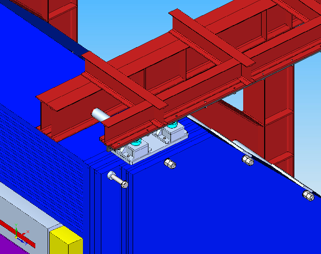
[General view] [Side view]

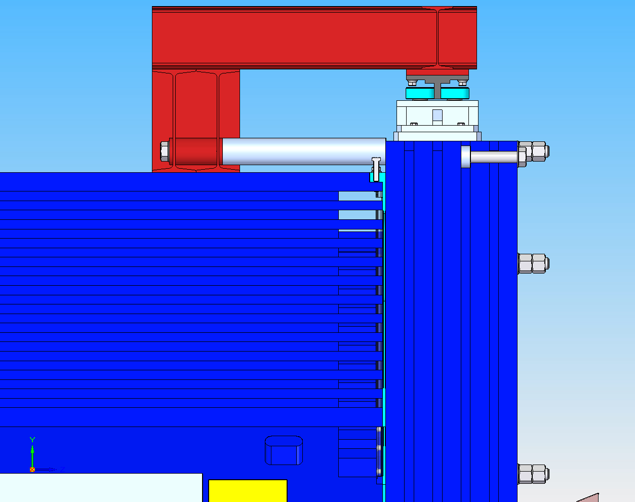
Figure 3.23: Upper part of the downstream end cap showing the guiding rollers for the door opening

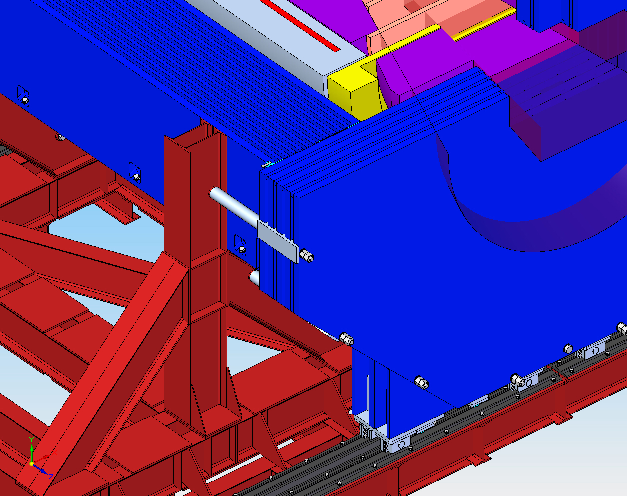
[General view] [Side view]

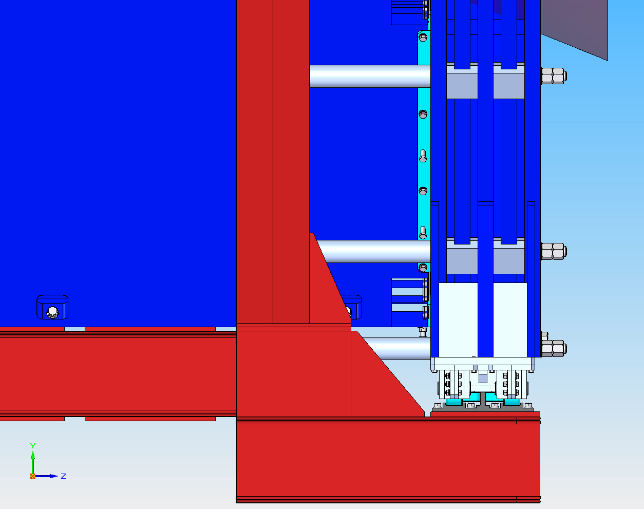
Figure 3.24: Lower part of the downstream end cap showing the load-bearing wheels for the door opening

Layer
Axially Outward	Thickness	$z_{min.}$	$z_{max.}$
from Centre	/ mm	/ mm	/ mm
1	60	2485	2545
2	60	2575	2635
3	60	2665	2725
4	60	2755	2815
5	60	2845	2905
TOTAL	300	2485	2905

Table 3.10: The axial iron lamination of the solenoid yoke forward doors, beginning from the innermost layer to the outermost.

This process led to the current design which complies with all requirements (see also Sec. 2.4.3) and enables to foresee a fall back solution for the Barrel DIRC, in which the slabs would be prolonged through the door and the readout box would be placed outside the flux return yoke.

The downstream doors will provide gaps to accommodate detectors, to be used as range system for the muons, similar to the barrel. Each doors consist of 5 steel plates, each of them being 60 mm thick. The plates are separated by means of 30 mm thick spacers and welded to each other. The positions of the spacers are shown in Fig. 3.22. The thickness and position of the downstream door will conform to the space requirements for the detectors placed inside it and close to it and to the magnetic field requirements in the tracker region. The downstream end cap will also effectively shield the stray fields of the solenoid into the Forward Spectrometer; and minimise fields at the location of the sensitive turbo-molecular pumps between the two spectrometers. The axial lamination is summarised in Table 3.10.

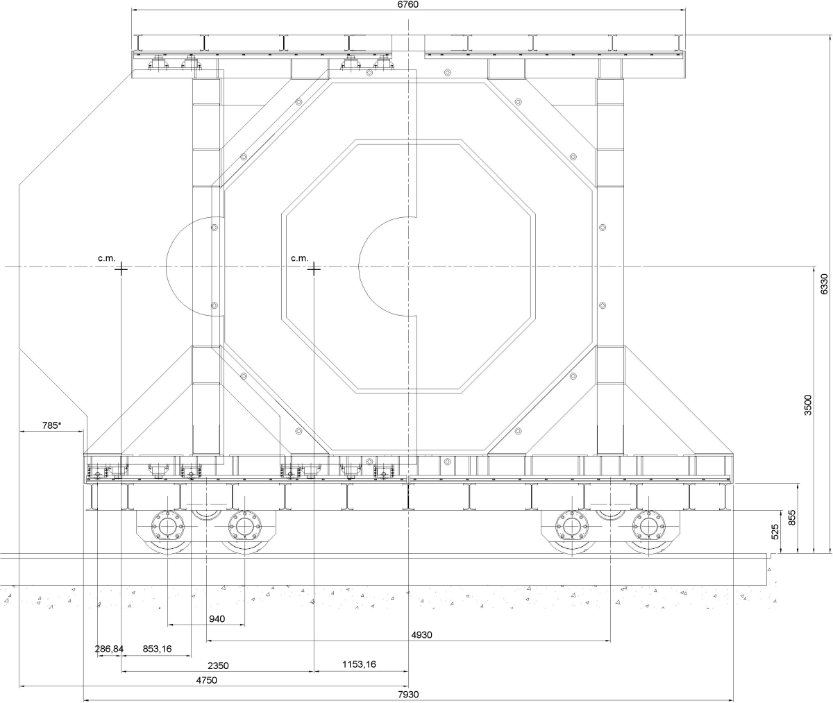
Figure 3.25: Front view of the solenoid yoke showing the maximum dimensions for the system with fully opened door and its centre of mass in both the closed and open position.

Door Opening System

Both the upstream and downstream doors will be mounted on rails, so that they can be opened reliably on a regular basis. A system of load-bearing wheels and horizontal guiding rollers will be mounted at the top and bottom of each door to provide the moving capabilities (see Figs. 3.23 and 3.24, respectively). The rollers systems for the upstream and downstream doors will be identical. In order to ensure a friction-less door opening spacers will be mounted on the faces of the barrel which can be (dis)mounted when the doors are closed. To further ease the opening procedure a 1 degree opening angle is foreseen with respect to the $x$ axis, i.e. $89^{\circ}$ w.r.t. the beam axis.

For safety reasons, the sliding doors will have to be fixed to the barrel by bolts during the magnet operation as well as during the transport of the whole solenoid from the assembly area to the in-beam position or vice versa. In the process of assembly and in the operation position, when the doors may be opened, there will be additional skid supports to bear the weight of the doors. The doors can be opened after removing the attachment bolts.

A front view of the solenoid yoke with dimensions for closed and fully open doors is shown in Fig. 3.25. The suspension has been designed in a way that stability is guaranteed both with closed and open doors, while keeping the space occupied by the support structure minimal for access at the in-beam position.

Weights of Yoke Parts

The total weight of the solenoid laminated flux return yoke will be 272 t. The weight of the carriage and of the space frames will be about 20 t. The weights of the yoke parts are given in the Table 3.11. The total weight of the iron for the solenoid will hence be 292 t.

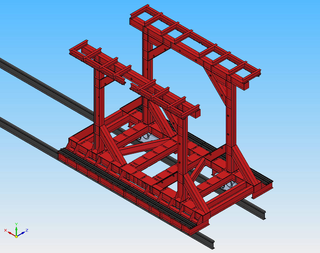
Figure 3.26: Solenoid support frames

Item	Weight
	$[$t$]$
Upstream door with
supports, wheels, rollers etc.
Left part	23.879
Right part	23.670
Total:	47.549
Octagonal barrel
Upper beam	20.117
Inclined side beams (4 pcs.)	22.298
Vertical side beams (2 pcs.)	22.298
Bottom beam	20.509
End face patch plates (16 pcs.)	0.243
Total:	178.302
Downstream door with
supports, wheels, rollers etc.
Left part	23.475
Right part	23.061
Total:	46.536
Support frames and carriage	19.685
Total weight of iron pieces:	292.072

Table 3.11: Summary of weights of the individual yoke parts in tons.

3.3.3 Support and Transport

Support Frame

To ensure the stability of the yoke and to ensure its geometry to remain precisely under control after long operation and many power cycles, an outside space frame is necessary. This will also ensure that sizable seismic loads can be withstood and hence the operational safety will be guaranteed. At the same time, this frame will allow the attachment of the opening mechanism and suspension of the doors. The frame will be welded from standard I-shaped steel beams and will be fixed by bolts to the outer beam plates. In addition it will improve the reproducibility of the solenoid yoke properties between the tests at the company and the final assembly on site.

The support frame will be integrated with the horizontal beams of the platform that will carry the total weight of the magnet. The vertical beams of the frame and the platform are constructed with IPE 330 beams (EURONORM 19-57, 330 mm in height, 140 mm in width) connected by arc welding and by bolts M20. The platform will be placed on 4 railing wheel carriages for transportation of the solenoid from the assembly position to the operation position in the experimental hall which is described below. A general view of the support frames is shown in Fig. 3.26.

Movement and Positioning

E. Lisowski, I. Lehmann

Conceptual Design

The design of the movement of the solenoid is based on the considerations in Sec. 2.4.3. As the whole system will weigh about 300 t these requirements pose a serious challenge to the design of both the support frame as well as the drive system.

A range of different options was considered. The favoured solution is based on the use of rails and wheels which can be driven directly in conjunction with a jacking system to align and suspend the system in both the operation position and the maintenance position. This solution seems advantageous compared to the use of Hilman rollers or air cushions. Both latter options require an additional system guaranteeing the precise and semi-automatic movement. In addition, the rail system is a reliable and conservative solution. The evaluation of the details and optimisation studies are still under way. Thus, the solution shown here has to be considered as conceptual only.

Studies using a 2-dimensional Finite Element Model (FEM) have been used to optimise the arrangement of support points. A solution with 6 support points at any operational position,i.e. the in-beam position and the maintenance position, and 4 support points during movement seemed favourable. A sketch of the conceptual design is shown in Fig. 3.27. The results of the FEM calculations for this solution are discussed in the following (Sec. 3.3.4).

Figure 3.27: Sketch of the concept for the drive and positioning system of the Target Spectrometer seen from upstreams. 1 – carriage, 2 – wheel, 3 – carriage support, 4 – carriage underframe, 5 – wheel, 6 – precise adjustable height support, 7 – lifting structure, 8 – central support.

The 4 identical carriages will have 2 wheels each and will be located directly under the vertical beams. The solution using levers in each carriage allows for an uniform load on each wheel during the movement. Once the desired position will have been reached the load will be taken by 6 precisely adjustable supports, 4 of which will be attached to the carriages and 2 additional ones at the centres of both main horizontal beams. Such, a support will be provided which imposes minimal deformations to the solenoid at the operational and maintenance positions. The deformation will stay within tolerable limits during the movement (see Sec. 3.3.4). The wheels will be subjected to the load only during the time of the movement. This will avoid wheel deformations which may occur when subjected to the load for long periods. In addition, this system will allow for a precise positioning of the solenoid with respect to an external reference frame. The lifting can be achieved using various solutions. The favoured solution is the use of computerised hydraulic jacks which can be mechanically locked as soon as the desired positioning will be achieved.

An artistic view from below the floor which illustrates the placement of the carriages on the support structure of the solenoid is shown in Fig. 3.28.

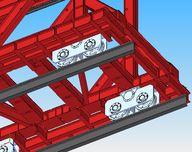
Figure 3.28: Details of solenoid movable platform and transportation carriage

Carriage Design

A model of a carriage with hydraulic jack in place is presented in Fig. 3.29. Each carriage will consist of two wheels with rims on both sides, a structure with joint (which will be fixed to the spectrometer frame), a cylinder (which will form the axis joint for the carriage and the structure), a gearbox, a brake and an electric motor. This structure will allow to get a uniform load on every wheel. Thus it is permissible to use a single motor and brake for a carriage. In our design we use 4 identical carriages, i.e. four electric motors and four gearboxes. The overall dimension of each carriage are planned to be $1.97\times 1.17\times 0.83$ m ($L\times W\times H$) including the gearbox and motor with a wheel diameter of 630 mm.

Figure 3.29: View of one carriage perpendicular to the rails at the operational position, where the weight will be taken by the jacking system: 1 – hydraulic cylinder, 2 – steel plates and mounting clamp resting on the support profile (invisible), 3 – foundation, 4 – carriage. The front steel plate of the carriage is shown as translucent to reveal the wheels and support inside the carriage. Gear box, brake and motor are hidden almost completely behind the carriage on the left side in this view.

Rail Tracks

Rails will be placed inside the floor in a way that their upper surfaces are level to the floor. The proposed rails are acc. DIN 1017, realised in St 70-2/E steel, welded on I profile HE300M acc. EN 10034:1994. Using special clamps covering the rails the whole load will be transferred to the I-profiles rather than the rails when the system will be lifted and during any period without frequent movement (see Fig. 3.30).

Figure 3.30: Cross section of the support profile (2) and rail (1) inside the foundation with dimensions given in millimetres.

Operating Data of Drive System

The drive system will consist of four electric motors, which motion is controlled in an open system by an electronic controller. The drive velocity can be smoothly changed.

The drive system data are anticipated as follows:

Wheel numbers	8
Driven wheel	4
Carriages	4
Electric motor	4
Spectrometer support	6
Lifting points	4
Controllers	1
Sliding friction coefficient	0.15
Adhesion friction coefficient	0.2
Wheel load	375000 N
Acceleration	0.1 m/s2
Deceleration	0.1 m/s2
Speed	1.5 m/min
Open loop control	1

3.3.4 Deformations and Stresses

Mechanical Analysis

An enhanced Finite Element mechanical analysis of the return yoke has been performed. The design criteria for the yoke and support frames correspond to the building norms and codes for steel constructions: Eurocodes 3 [EuroCode3].

Material Properties

The material to be used for all modules will be low carbon steel AISI 1010 (DIN 1.1121). The chemical composition of this steel is given in Table 3.12, and the mechanical properties in Table 3.13. The dependence of the magnetic induction $B$ on the magnetisation field $H$ in the material is shown in Fig. 3.5.

C	Si	Mn	S	P	Cr	Ni	Cu	N2
0.07-0.14	0.17-0.37	0.35-0.65	0.04	0.035	0.15	0.25	0.25	0.08

Table 3.12: Composition of elements alloyed with iron in AISI 1010 steel, in %.

Item	Value
Coefficient of thermal
expansion at 18∘C, degree-1	$1.3\cdot 10^{-5}$
Young’s modulus, GPa	198
Tensile strength
(annealed sample) $\sigma_{u}$, MPa	340
Yield stress of
annealed sample $\sigma_{y}$, MPa	210
Elongation, %	29

Table 3.13: Mechanical properties of AISI 1010 steel.

Magnetic Forces on the Doors

The axial magnetic force acting on the upstream door will be $1.85\,$MN in total. The downstream end cap will be subjected to a total axial magnetic force of $-1.40\,$MN.

The forces acting on the downstream end cap plates are given in Table 3.14. The strength of the force imposes additional constraints on reinforcement of the end cap plates. This reinforcement must not prevent insertion of the muon chambers.

Plate No.	$F_{z}\,[\unit{kN}]$
1	-816.7
2	-379.9
3	-178.1
4	-27.1
5	-0.3

Table 3.14: Axial forces expected to be acting on the iron plates of the downstream end door.

Deformation of the Yoke

Deformation of the yoke in its cross section is calculated for three load cases:

1. gravity load G = G₁ + G₂ + G₃ = 3460 kN, where G₁ = 2050 kN – the weight of the yoke barrel with support frames, G₂ = 410 kN – the weight of the cryostat with attached detectors and G₃ = 1000 kN – the weight of the end caps;

2. gravity load and magnetic forces;

3. gravity load, magnetic forces and additional vertical and horizontal seismic loads $P_{y}=0.11\unit{G}$, $P_{x}=0.15\unit{G}$.

Both 2D and 3D finite-element models (FEM) were used to calculate the deformations and stresses. The 2D yoke model is shown in Fig. 3.31. It should be noted here that the simplifications which went into this model ensure that the results can be treated as a worst case scenario, and the full system would deform no more than this model predicts. The iron yoke plates are loaded by magnetic pressure, non-uniformly distributed over their surface according to the radial component of magnetic induction (see Fig. 3.32).

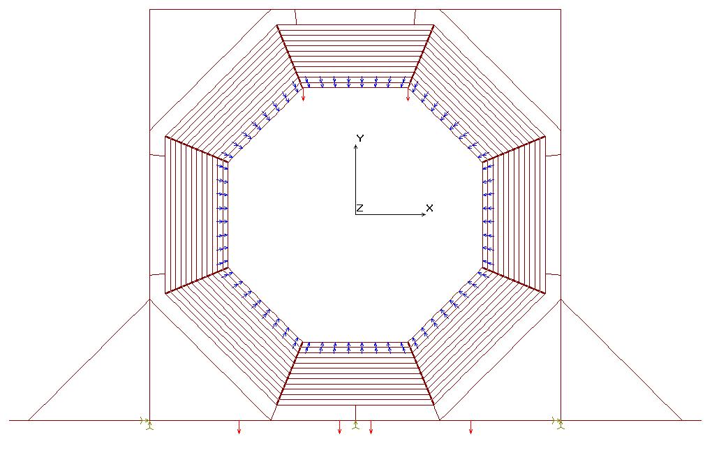
Figure 3.31: 2D FE yoke model showing application of the doors, cryostat and detectors weight (red arrows), magnetic pressure (blue arrows), outer support frame and fixation points at the basement

Figure 3.32: Distribution of $B_{R}$ along the inner surface of the yoke beam ($R=1490\,mm$)

Figure 3.33: Deformation of the yoke due to gravity in the stationary positions, i.e. using 6 support points.

Deformation due to Gravity

The yoke frame will be placed on the platform, which will be supported at 6 points on its footprint in the solenoid assembly and final positions. It could be shown that the deformations will be minimal when placing the support points under the vertical beams and the centre of yoke at both support frames.

In the stationary position, the yoke gravity load will result in the maximal vertical height change within the yoke, which is calculated to be $\Delta y=1.3\unit{mm}$. The maximal horizontal change of width inside the yoke will be $\Delta x=2.4\unit{mm}$ (see also Fig. 3.33).

When the supports will be removed in order to allow the movement of the system, the platform will remain on the wheels for transportation. In effect this means that the two central support points will be released while the outer 4 points will stay under load (see Fig. 3.34). In this case the situation will be less ideal than in the stationary position but the deformations will remain within tolerable limits. We still investigate additional reinforcements of the support frame which may reduce the deformations further.

Figure 3.34: Deformation of the yoke due to gravity during the movement, i.e. using 4 support points.

When the solenoid is being transported, the doors have to be closed and rigidly attached to the barrel part. After the magnet is moved to its operation position at the beam line, the platform is supported on the supports again.

Deformations due to Magnetic and Seismic Loads

The first (inner) plate will be loaded by a magnetic force of $105.8\unit{kN}$, the second plate by $20.9\unit{kN}$. The maximal vertical and horizontal deformations due to gravity load and magnetic pressure are calculated to be: $\Delta y=1.9\unit{mm}$, $\Delta x=\pm 1.1\unit{mm}$.

The estimated deformations of the yoke barrel beam due to magnetic pressure (additional deformations when the magnet will be switched on) are shown in Fig. 3.35. The deformations are calculated at the cross-section near the barrel ends in the area where the magnetic pressure will be maximal. The deformation will be less than 0.2 mm. It will not change the positions of the octagon corners, but the shape of the inner plates of the beam.

Figure 3.35: Deformation of the yoke beam plates due to magnetic pressure.

In case of combined action of gravity, magnetic and seismic loads the maximal vertical height change within the yoke will be $\Delta y=1.8\unit{mm}$. The maximal horizontal change of width inside the yoke will be $\Delta x=2.7\unit{mm}$ (see Fig. 3.36).

Figure 3.36: Deformation of the yoke due to gravity, magnetic and seismic loads.

In our design the outer support frame significantly increases the general rigidity of the yoke. Not using the frame would lead to a yoke deformation $\Delta y>7\unit{mm}$.

Figure 3.37: Von Mises stress in the body of carriage in MPa

Figure 3.38: Total deformation of the body of the carriage in mm

Figure 3.39: Von Mises stress in the central support of carriage in MPa

Rail Carriages and Supports

E. Lisowski, I. Lehmann

Full 3D FEM calculations were performed for all crucial components of the carriage and support system, i.e. the frames of the carriages with their hinge and support structures, the wheels and their impact on the rail/I-profile, and the clamps used to suspend the weight during operation and their impact on the rail/I-profile.

Frame of the Carriage and Central Support

When the solenoid is to be moved the weight will rest on the 4 carriages. The following data were used in the FEM analysis:

1. force acting on support $F=80\unit{tonnes}$;

2. contact connection between pin and support and between pin and frame of the carriage;

3. material: steel.

FEM results for the carriage and the central support are shown in Figs. 3.37, 3.38 and 3.39, respectively. Stress values are below permissible levels, and the maximum displacement does not exceed 0.5 mm.

Wheel and Rail

The 8 wheels will transfer the weight to the rails. The following data were used in FEM analysis:

1. force acting on support $F=40\unit{tonnes}$;

2. contact connection between rail and wheel and between wheel and its axis and support and pin with frame of the carriage;

3. material: steel.

FEM results are shown in Fig. 3.40 and Fig. 3.41. Stress values are below the permissible levels and the maximum displacement is $\sim 0.1\unit{mm}$.

Figure 3.40: Von Mises stress for wheel-rail model in MPa

Figure 3.41: Total displacement in mm

Clamp on I Profile

A clamp which will rest on the I profile below the rail will be used whenever the system is supported on jacks. The following data were used in FEM calculations:

1. force operating acting on support $F=80\unit{tonnes}$;

2. contact connection between clamp and rail;

3. material: steel.

FE results are shown in Fig. 3.42 and Fig. 3.43. Stress values are below the permissible stress levels and the maximum displacement is $\sim 0.2\unit{mm}$.

Figure 3.42: Von Mises stress in rail and support

Figure 3.43: Total displacement in rail and support

Deformation of the Upper Yoke Beam

The 3D model of the upper beam includes 13 steel plates with recesses for the target and for the chimney (Fig. 3.44). In this model the plates are consolidated by means of $30\times 30\unit{mm}$ steel spacers along the side surfaces of the beam using the weld seam. The magnetic pressure is applied to the first two inner plates of the beam. Besides that, the beam is loaded by the axial force $F_{z}=0.23\unit{MN}$ acting at the beam butt-ends from the yoke end caps.

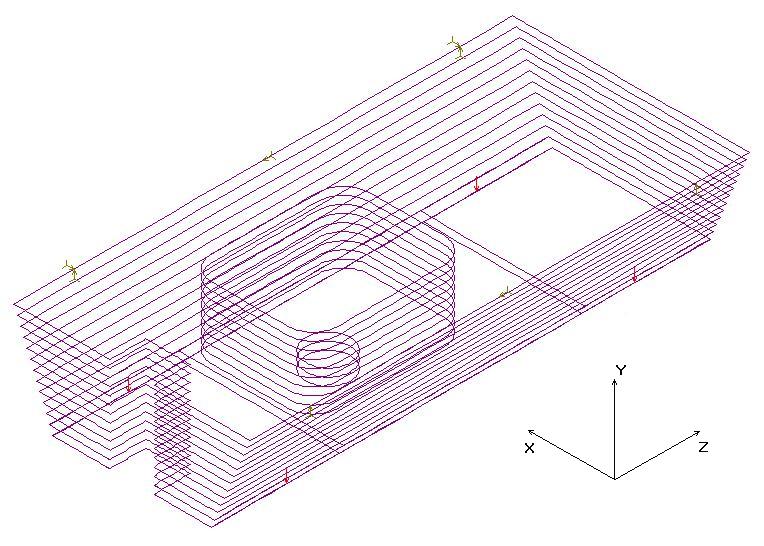
Figure 3.44: 3D FE model of the upper yoke beam showing the points of application of cryostat and detectors weight and points of fixation

The results of computations of deformations due to gravity (without cryostat) show that the maximal deflection is $0.3\unit{mm}$. The deformations due to gravity (with cryostat and detectors) and magnetic forces are shown in Fig. 3.45. The resulting maximal vertical displacement is $0.6\unit{mm}$. That means that the beams will rigid enough; their sags will be comparable with the accuracy of manufacturing.

Figure 3.45: Upper beam deformation due to gravity and magnetic forces

Stresses in the Yoke and Support Frame

According to our calculations the equivalent (Von Mises) stresses in the yoke beams are within allowable limits $[\sigma]=140\unit{MPa}$ and the stresses in support frames are $\sigma<100\unit{MPa}$ both including and excluding the seismic load. The distribution of stresses in the upper yoke beam due to gravity and magnetic forces is shown in Fig. 3.46.

Figure 3.46: Von Mises stress in the upper yoke beam due to gravity and magnetic forces

The details of the stress distribution in the upper yoke beam are shown in Fig. 3.47. The stresses will have local maxima at the fixation points, where the concentrated force will be applied.

Figure 3.47: Details of the stress distribution in the upper yoke beam

The material resistibility class of bolts consolidating the yoke beams is foreseen to be 10.9. This resistibility will be sufficient for calculated tensile loads $<40\unit{kN}$ per bolt M24.

Deformations and Stresses in the Downstream End Cap

The 3D model of the downstream door is shown in Fig. 3.48. The connection of the plates is realised through the welded spacers along the side surface and through the horizontal welded spacers.

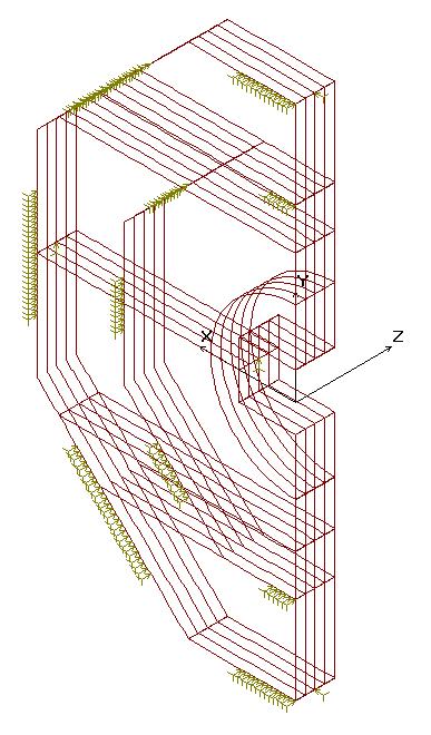
Figure 3.48: 3D model of the downstream door

Axial deformations of the downstream door due to magnetic force are shown in Fig. 3.49. The maximal value of the displacement is obtained to be $\Delta Z<0.3\unit{mm}$. The deformation depends on the number of welded spacers used to connect the neighbour steel plates. The dependence of deformation on the number of additional (besides that at the periphery) horizontal spacers is presented in Table 3.15. The solution with three spacers is regarded as optimal. The stresses in the downstream door are shown in Fig. 3.50. The maximal value of the stress is anticipated to be $\sigma<30\,MPa$.

Figure 3.49: Deformation of the downstream door

Number of	Maximal bending
welded spacers	deflection [mm]
No spacers	8.1
1 spacer	1.1
3 spacers	$<0.3$

Table 3.15: Axial bending deflection of the second plate of the downstream door

Figure 3.50: Von Mises stresses in the downstream door

Deformations and Stresses in the Upstream End Cap

Axial deformations of the upstream door due to magnetic force are shown in Fig. 3.51. Axial displacements along the line 0-1 are shown in Fig. 3.52. The maximal value of the displacement is calculated to be $\Delta z<3\unit{mm}$. The stresses in the upstream door are shown in Fig. 3.53. The maximal value of the stress is calculated to be$\sigma<12\unit{MPa}$.

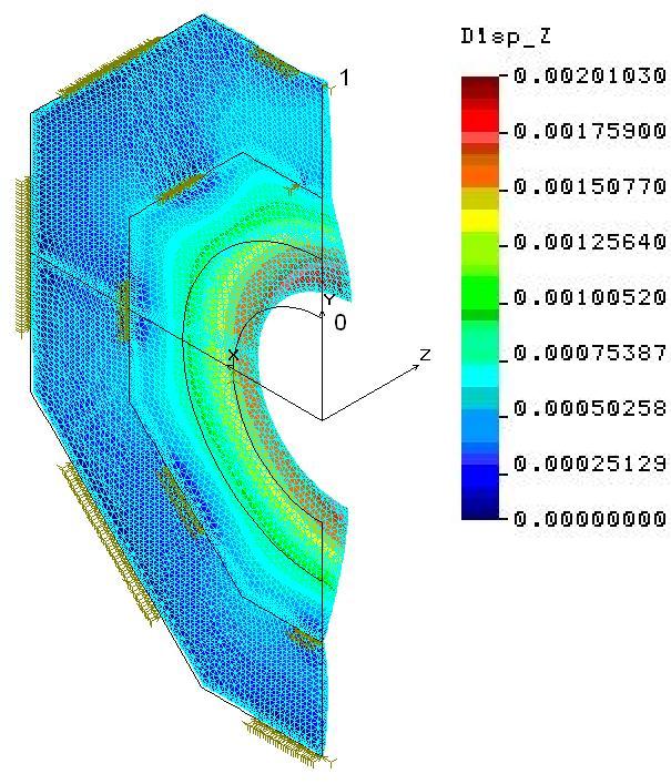
Figure 3.51: Deformation of the upstream door

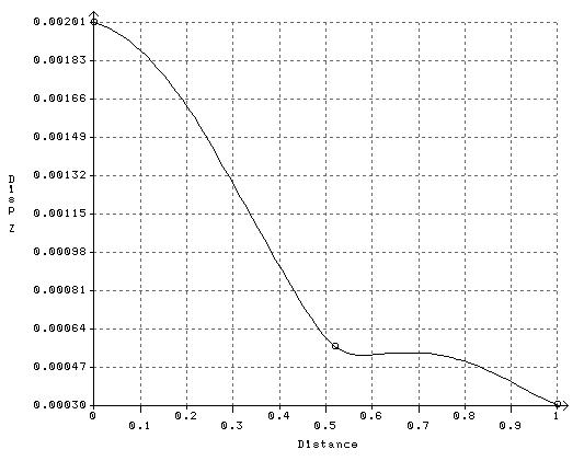
Figure 3.52: Axial displacement [m] of the upstream door along the line 0-1 (Fig. 3.51)

Figure 3.53: Von Mises stresses in the upstream door

3.3.5 Assembly of the Yoke

The assembly of the flux return yoke in the hall will be done in the service area, where sufficient space for detector installation is foreseen. The structures and the iron segments will be delivered through an opening in the hall roof. The movement of the single yoke elements, whose weight will be $\sim 20\unit{t}$, will be done using the overhead crane and, if needed, additional mobile cranes operated from outside the experimental hall.

The process of assembly will start with the installation of the lower part of the magnet support system. The platform of the magnet will be mounted on temporary supports to provide stability of the construction. (The wheels of the platform will be in a lifted state at this stage.) These supports are the same which will also be used to support the magnet in its operation position at the beam line.

The 4 vertical beams of the yoke support frame will be mounted on the platform. The lower knees supporting the vertical beams will be installed.

The lowest beam of the yoke barrel will be placed on the platform. Then the 2 inclined lower beams will be installed and attached to the horizontal one by temporary screwing. Then the template frames that control the form of the internal boundary of the yoke will be mounted.

The side (vertical) beams of the barrel will be installed and attached by temporary screwing. The inclined upper barrel beams will be placed on them. Then the upper knees supporting the outer frame will be mounted. The upper barrel beam will then be installed and attached by temporary screwing. The final fastening of the attachment bolts in the barrel beams will be performed.

The 2 upper crossbars of the outer frame will be placed on the vertical bars with the knees. The outer frame will be attached to the barrel by bolts. The internal template frames will be removed and the geometric parameters of the yoke will be checked.

The barrel end caps will be installed on their rails at the solenoid platform. The upper guide frames for the end caps will be mounted and the door adjustment will be performed. As final test, the door opening mechanism will be checked.

3.4 Performance

A. Bersani, Y. Lobanov

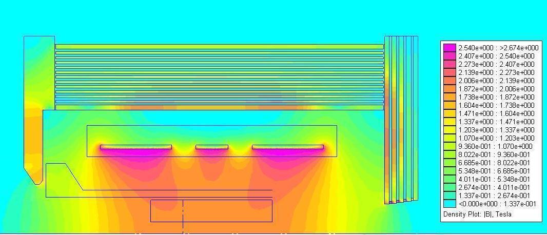
Figure 3.54: Magnetic flux density distribution (cross section for half of the horizontal plane where the beam comes in from the left). The iron yoke, coil and cryostat, the barrel DIRC and the outer tracker are indicated by their outlines.

3.4.1 Introduction

The optimisation of the solenoid magnet design was performed by independent groups using different techniques and software, both for finite elements modelling [Efremov:2008, Bersani:2008], and for subsequent analysis [Koshurnikov:2006]. The final field maps were calculated using the TOSCA code [mag:TOSCA_2003] in a complete 3D model with the dipole magnet operated at different energies.

As stated above, the coil position and the flux return yoke will not be symmetric: this will lead to an unbalanced magnetic force directed parallel to the beam line. An effort was spent to minimise this residual axial force, optimising the winding geometry. The final design features a residual unbalanced axial force of $2\cdot 10^{5}\unit{N}$ directed from downstream to upstream with respect to the beam direction. This force is very sensitive to the displacement of the coil with respect to its nominal position. The force derivative w.r.t.  displacement will be $4\cdot 10^{4}\unit{N/cm}$, increasing in the direction of displacement. The support structure and structural calculation were performed with a safety factor of 4.

The final design is fully compliant with all magnetic requirements, mechanical constraints and technical guidelines that were described in the previous sections. The key aspects of the magnet performance in terms of fields, operation and beam interference are described in the following.

3.4.2 Field in Tracker Region

The calculation of magnetic fields and forces has been performed in the framework of axially-symmetric and 3D FE models, with different detail level and different symmetry properties in the different phases of design optimisation. A distribution of the solenoid magnetic flux density, obtained with an axial-symmetric model and about $10^{6}$ elements is shown in Fig. 3.54.

In the optimised solenoid design we have achieved that the field inhomogeneity, i.e. the deviation $\Delta B/B_{0}$ from the nominal field $B_{0}=2$ T, stays below $1.6\%$ in any point within the outer tracker. See also Fig. 3.55. This undershoots the request of $\Delta B/B<2\%$ significantly. The field is even homogeneous to better than $\pm 1\%$ in more than $90\%$ of the tracker volume. The resulting calculated distribution is homogeneous to the per mile level in the central region of the tracker, i.e. $-200\leq z\leq+800$ mm. The peaks at the corners cannot be avoided if keeping to the mechanical constraints from the detectors on the geometry of the cryostat.

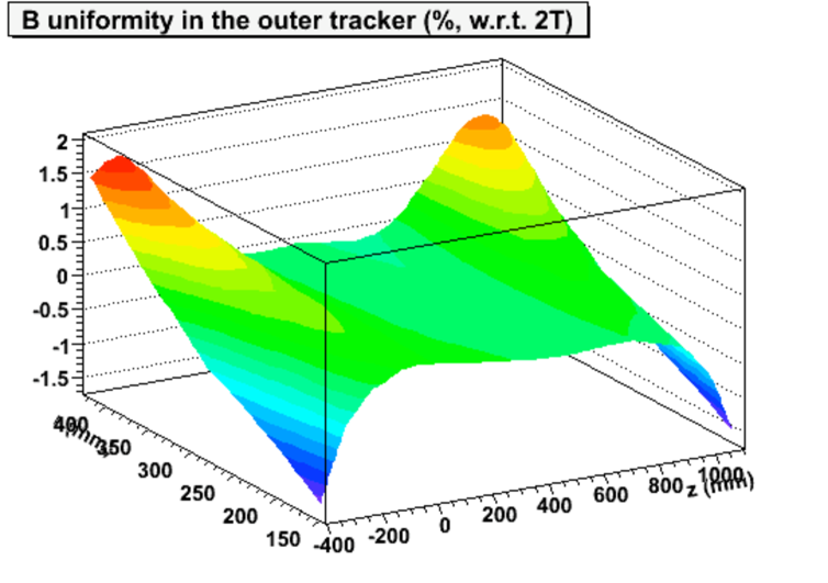
Figure 3.55: Field homogeneity $\Delta B/B$ in the outer tracker region. The radius from the target $r$ and the coordinate along the beam direction $z$ are given on the lower axes in millimetres. The vertical axis shows the relative difference between the nominal field $B_{0}=2$ T and the actual field in this coordinate in per cent.

The design also fulfils the requirements concerning the integral of the radial component of magnetic induction field:

$$I(r,z_{0})=\int\limits_{-400}^{z_{0}}B_{r}(r,z)/B_{z}(r,z)\,dz<2\,mm.$$

for $150\unit{mm}\leq r\leq 420\unit{mm}$ and $-400\unit{mm}\leq z_{0}\leq 1100\unit{mm}$, i.e. in the outer tracker region. The optimised design gives $0\unit{mm}\leq I(r,z_{0})\leq 2\unit{mm}$ for any given value of $r$ and $z_{0}$. In addition, only positive values of $I(r,z_{0})$ and a smooth behaviour is achieved. This is especially crucial for the operation of a Time Projection Chamber (TPC). A plot of the $I(r,z_{0})$ distribution in the outer tracker region is shown in Fig. 3.56.

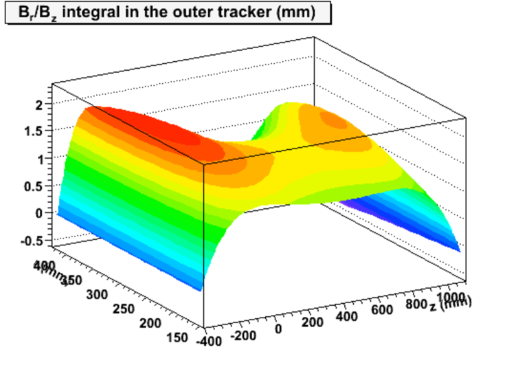
Figure 3.56: Integral of radial field component $I(r,z_{0})$ in the outer tracker region. The radius from the target $r$ and the coordinate along the beam direction $z$ are given on the lower axes in millimetres. The vertical axis shows $I(r,z_{0})$ (see text) in millimetres.

3.4.3 Fringe Field and Field in Flux Return

Particular care was taken during the design development on the fringe fields near the return yoke apertures and in the return yoke itself.

The fringe fields will be critical in several regions:

1. DIRC readout regions;

2. slits for cables and services in the barrel;

3. target recess in the upper octant;

4. outside the yoke on the beam axis.

Problems can arise due to photon detectors operation (point 1), insufficient iron cross section and local increase of magnetic reluctance (point 2) or turbo-molecular pumps operation (points 3 and 4). Every region was separately studied.

The field in the iron flux return yoke and in the doors was studied to evaluate the development of saturation in the most crucial regions. This was done in an iterative process in order to minimise the saturation of the iron. It is advisable to keep saturation low, as this enhances the magnet’s efficiency, strong local field distortions may appear close to saturated parts, and nonlinear effects which are difficult to control appear in forces and fields.

Magnetic Field in the DIRC Readout Region

The barrel DIRC readout will be installed inside the iron yoke and will be read out with the recently developed Micro-Channel Plate Tubes (MCPTs). These devices are almost insensitive to magnetic field up to 1 or $1.5\unit{T}$, depending on the models and dimensions of the sensitive area. The flux density distribution in this area is shown in Fig. 3.57.

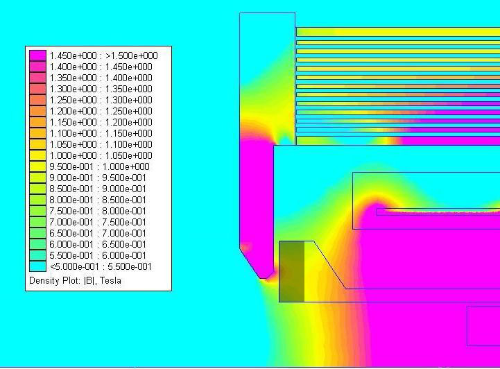
Figure 3.57: Magnetic flux density in the region of the Barrel DIRC readout. The MCPTs will be located on the left within the grey-shaded box depicted here. The field there will remain below 1 T.

Due to the optimisation of the upstream end cap, the flux density in the area where the MCPTs will be operated is $|B|<1\unit{T}$. Since the technology of MCPTs is relatively new, we foresee a backup solution where the slabs extend outside the end cap. Here the readout would be in a region of much lower fields of few $\unit{mT}$ and could be even shielded easily further.

Effect of Cable Routing

Cut outs in the return yoke barrel are foreseen to allow the feed-through of most of the cables and service lines for the detectors. The size of each slit will be $140\times 420$ mm² and there will be one at each corner of the octagon both at the upstream and downstream ends of the barrel (see Fig. 3.4).

The effect of the cut outs on the field parameters has been extensively studied. Although the magnetic field in the area of the passages will be disturbed due to redistribution of flux, its influence on the field in the central region will be insignificant. This conclusion has been confirmed using complete 3D magnetic field calculations within the model shown in Fig. 3.6 that takes into account the actual shape and dimensions of recesses in the yoke barrel. The results of calculations of the field inhomogeneity and of the integral of the radial component of magnetic induction (see Fig. 3.55 and Fig. 3.56) show that the requirements on the field quality are satisfied.

[$y-z$ plane, $x=0$] [$x-y$ plane, $z=0$]

Figure 3.58: Flux density in the target recess. The field sensitive turbo-molecular pumps will be located at a height of 2.0 m from the beam, i.e. at the level of the $x$ or $z$ axis in the plots.

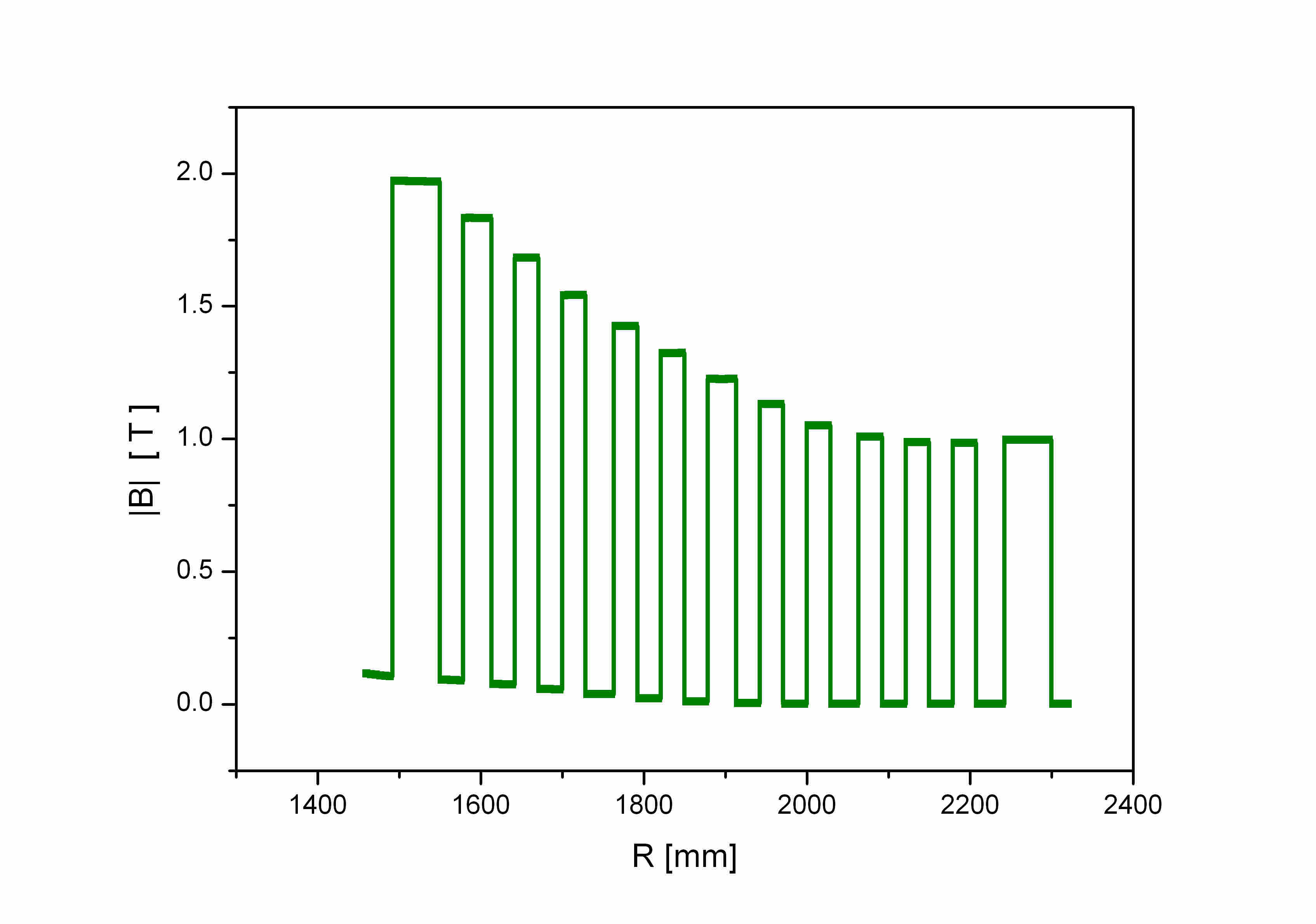
[Barrel ($Z=1300\,$mm)] [Downstream end cap ($R=1200\,$mm)]

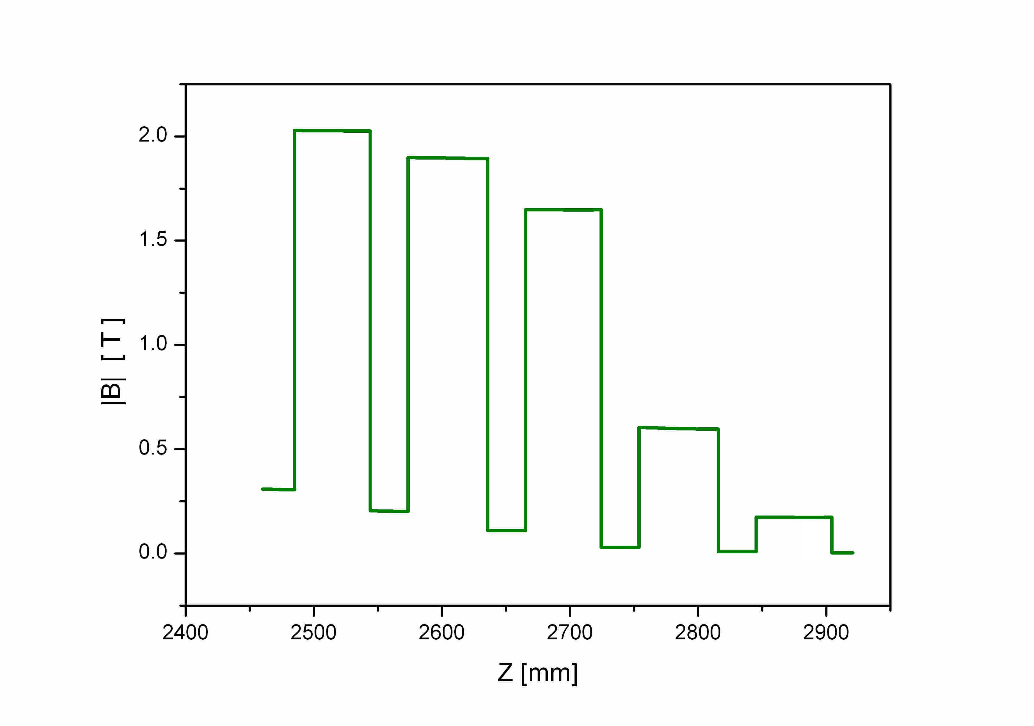
Figure 3.59: Flux density in different parts of the yoke.

Stray Fields Outside the Yoke

The magnetic flux distribution in the recess for the target has been studied, because the generator of the target requires turbo-molecular pumps, which should be located at a height of 2.0 m from the beam and could safely tolerate fields of 5 mT, but not much higher. The plots of this distribution in the vertical $y-z$ plane (containing the beam axis) and in the $x-y$ plane (perpendicular to the beam axis) are shown in Fig. 3.58 and Fig. 3.58. The requirement that in the region of the turbo molecular pumps the magnetic field must not exceed 5 mT is clearly satisfied.

A smaller recess is foreseen in the lower octant, where the turbo-molecular pumps will be placed further away from the interaction point. This recess will have no large effects, neither from the viewpoint of fringe fields nor from the inducted field distribution.

Downstream from the solenoid the pumps in this region will be placed more than $1\unit{m}$ off the centre of the beam pipe. The stray field outside the flux return yoke will anyhow be well damped in downstream direction as the orifice in the door will be relatively small. Thus no problem from fringe fields arises here. In contrast to that in upstream direction, since the opening will be relatively large and the door will be relatively thin, a slightly higher fringe field will arise. This poses no restriction though, as the cable and supply routing to the inner detectors and the EMC end plug will inhibit the installation of turbo-molecular pumps closer than $60\unit{cm}$ to the door anyway. At this distance also in that region the field will be tolerable for such pumps.

Magnetic Induction in the Iron Yoke

The yoke lamination makes the flux line distribution more complex than a compact flux return yoke. There is the possibility that high saturation arises locally, generating deformations of the flux line distribution near the iron.

Two cases where studied in particular:

• the barrel yoke near to the first and last sub-coil;

• the downstream door near the beam pipe hole.

In both cases, small volumes where the flux densities reach $2\unit{T}$ are found. These regions, however, will be extremely limited in size. It was, furthermore, demonstrated that they have no significant effect. Two plots of the density profiles in the barrel yoke and in the downstream door, where the highest values were calculated, are shown in Figs. 3.59 and 3.59.

As a result of the optimisation of the upstream door design, the maximum value of magnetic induction in it is calculated to be $|B|<1.8\unit{T}$, so there will be no saturation effect in the upstream door.

3.4.4 Solenoid Operation

The solenoid magnet has been designed and optimised to work at $2\unit{T}$ central field and $5000\unit{A}$ current, but it can be easily operated at lower currents. Operation at 60-80% of the maximum current is foreseen to allow stable accelerator operation at low beam momentum. In this case the solenoid’s performance in terms of homogeneity will be worse, but only slightly. Usually, the magnet will be ramped up at the beginning of a measurement period and remain at its current setting for the whole period, typically for up to half a year. Whenever required, it can be ramped up or down within about half an hour.

Transient Behaviour

Normal Power Cycling

Power cycling of the solenoid was studied to find the optimal compromise between energization speed and thermal dissipation. A calculation was performed using a 3D Finite Element Model (FEM) with the Ansoft Maxwell code [coil:maxwell]. The result is that the power dissipation due to eddy currents in the coil former can be kept under $10\unit{W}$ assuming a ramp up time of $2000\unit{s}$, or, in other words, a current rise rate of $2.5\unit{A/s}$. The current ramp and the power dissipation are plotted in Fig. 3.60.

Figure 3.60: Power loss via eddy currents in the coil former during normal power cycling as a function of time.

Current $[\unit{A}]$)	5000	4000	3000	2000
Central Induction	$2\unit{T}$	$1.6\unit{T}$	$1.2\unit{T}$	$0.8\unit{T}$
Conductor Peak Field	$2.8\unit{T}$	$2.4\unit{T}$	$2\unit{T}$	$1.5\unit{T}$
$I(r,z_{0})$ in the Tracker $[\unit{mm}]$	$0<I<2$	$0<I<2$	$0<I<2.1$	$-0.1<I<2.1$
Uniformity in the Tracker	$\pm 1.6\%$	$\pm 1.8\%$	$\pm 2\%$	$\pm 2.1\%$
Stored Energy	$21\unit{MJ}$	$14\unit{MJ}$	$7.7\unit{MJ}$	$3.4\unit{MJ}$

Table 3.16: Main field parameters of the  solenoid at different current settings. A setting between 3 and 4 kA is envisaged for the operation at low beam momenta.

During power cycling, the force will increase following a quadratic dependence w.r.t. the current. This is true only if non-linear effects from the induction will stay negligible. As discussed above, some small saturated regions are expected both in the yoke barrel and in the end doors. This saturation may induce deviations to the theoretical behaviour. However, it could be shown by calculations that in solenoid magnet the deviations from the pure quadratic law will be negligible (see Fig. 3.61). The relevant aspect of this calculation is that the residual axial force is a steadily increasing function during solenoid energization. This feature of the axial force allows a simpler design of the suspension system of the coil in the cryostat and of the cryostat in the yoke, compared to a situation in which the force is almost balanced but can change direction during power cycling.

Figure 3.61: Residual axial force as a function of current during normal power cycling. The force will increase steadily and will never change direction.

Emergency Shutdown

In case of a quench of the magnet, the quench protection system will open the quench switches and the solenoid will discharge on the protection resistor, according to the circuit shown in Fig. 3.10. Since the inductance of the solenoid will be $1.7\unit{H}$ and the resistance of the protection resistor will be $0.1\Ohm$, the discharge time constant will be $17\unit{s}$. This means that the current will need few of seconds to reach a value in the order of $100\unit{A}$, at which the solenoid can be considered switched off. In these $30-60\unit{s}$ approximately $60\%$ of the stored magnetic energy will be dissipated in the protection resistor and the remnant will be transformed into heat in the coil. The time dependence of the power dissipated in the coil former is shown in Fig. 3.62.

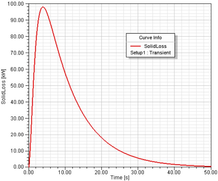
Figure 3.62: Power loss via eddy currents in the coil former during a quench.

The heat which will be generated in the coil former is sufficient to spread the quench all over the coil. The maximum temperature that will be reached in the coil will stay below $80\unit{K}$. This is comparable to magnets of similar type and poses no difficulties. It is anticipated that, after a quench, the whole cold mass will be at the temperature of the radiation shield or below, i.e. at $<60\unit{K}$. This will allow to proceed with a normal cooling procedure with liquid helium after a quench.

Reduced Current Operation

During the operation at beam momenta below 2.25 GeV/c the solenoid will be operating at a reduced current between 60 and 80% of the full current to reduce tune shifts in HESR. For this reason, the magnet performance was evaluated at currents lower than the engineering current. A summary of the main parameters for various different currents is shown in Table 3.16.

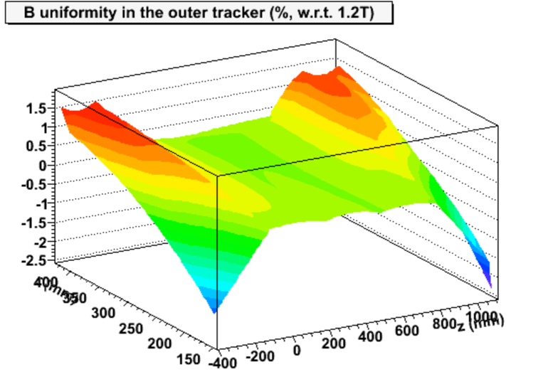
Figure 3.63: $\Delta B/B$ distribution over the outer tracker region at $60\%$ of the nominal current.

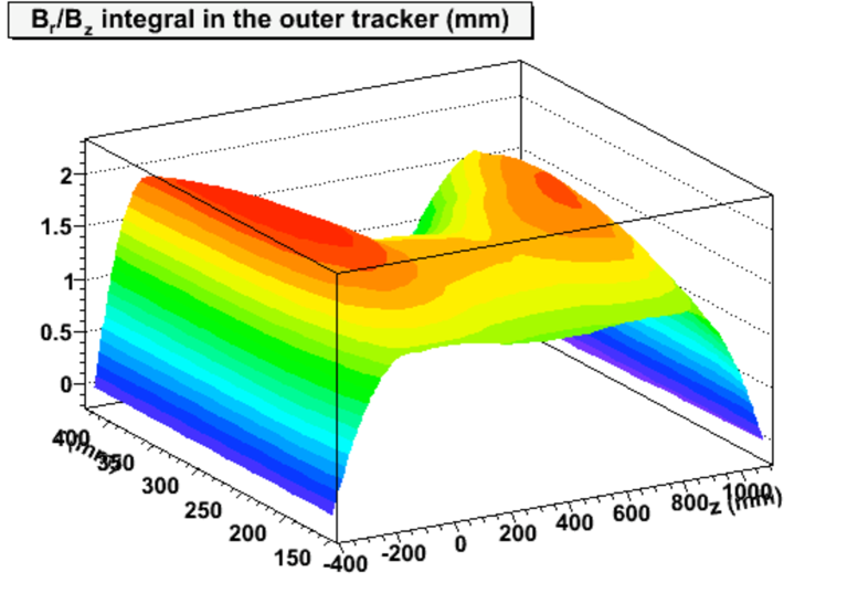
Figure 3.64: $I(r,z_{0})$ distribution over the outer tracker region at $60\%$ of the nominal current.

Since the material properties are not linear the magnetic field will not simply scale with the current. Due to that a small increase in the $I(r,z_{0})$ integral needs to be accounted for at lower currents. The distributions of $\Delta B/B$ and $I(r,z_{0})$ in the outer tracker region are shown in Fig. 3.63 and in Fig. 3.64, respectively. This should be compared with the distribution obtained at the engineering current, which were shown in Fig. 3.55 and Fig. 3.56.

Field Mapping

Field mapping will be performed using existing equipment at GSI and with the help of the GSI Magnet Technology Group. It is envisaged that one full 3D field map would be determined for two current settings: at the full field and one lower field setting, the latter allowing the operation at lowest beam momenta. This work will be performed as soon as the magnet is fully commissioned. Interpolating between the grid points and maps will allow us to determine the magnetic field at every point in the spectrometer opening and any current to sufficiently high accuracy.

3.4.5 Influence on the HESR Beam

The solenoidal field will influence the beam in two ways. Firstly the beam optics will be affected even in an ideal configuration. This will be dealt with by a counter-solenoid placed in front of the PANDA solenoid, which will be provided from the accelerator side. Here we discuss only the effects on the beam slope and mean position due to possible alignment errors.

To first order, the HESR antiproton beam will pass through the centre of the superconducting solenoid magnet, and the antiproton beam will be parallel to the solenoid axis. In this ideal scenario there will be no interaction between the beam and the magnetic field. However, in reality, the magnet alignment will not be perfect. An imperfect magnet alignment generates a small magnetic field ($B_{p}$) perpendicular to the beam trajectory which bends the beam by a small angle and shifts the beam trajectory away from its nominal position, i.e. generating an orbit error. It will not be easy to achieve a magnet alignment better than a few milli-radians due to its large weight and size. Another important reason for the misalignment is that there is always a difference between the magnetic central line and the mechanical central line, and even the magnetic central line does not strictly follow a straight line. Since the magnet misalignment can happen in any direction, the orbit errors may occur in both horizontal and vertical directions.

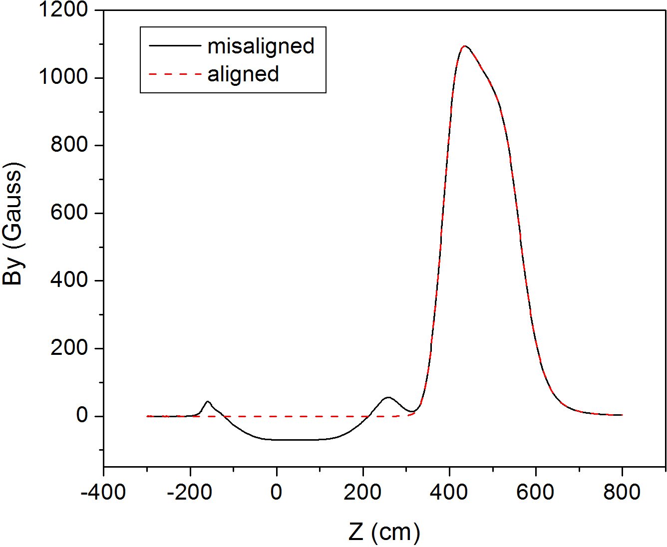
Figure 3.65: Field along the central line for an aligned solenoid (red dashed line) and misaligned solenoid by 0.2 degrees (black solid line). In this calculation the dipole has a field integral of $\sim$0.2 Tm and the antiproton momentum is 1.5 GeV/c.

In order to quantitatively understand the orbit errors caused by the spectrometer, 3D Tosca magnetic field calculations were carried out. In these calculations, both the solenoid and the Forward Spectrometer dipole magnet are modelled. A small polar angle misalignment of $0.2^{\circ}$ ($\sim$3.5 mrad) is considered. For simplicity, the solenoid is rotated around the x-axis. The coordinate system used here is the coordinate system. The x-axis is in the horizontal plane and perpendicular to the antiproton beam, the y direction is the vertical direction and the z axis is along the incoming antiproton beam direction. The magnetic field in the centre of the solenoid is set to be 2 T. To make the calculated field as accurate as possible, around 2 million nodes are used in the Tosca calculations. Based on the calculated fields, beam trajectories are calculated for different beam energies. Because of the extension of the Forward Spectrometer detectors the orbit errors are estimated at $z=10\,$m.

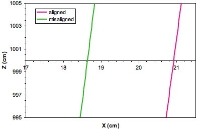
[1.5 GeV/c beam] [15 GeV/c beam]

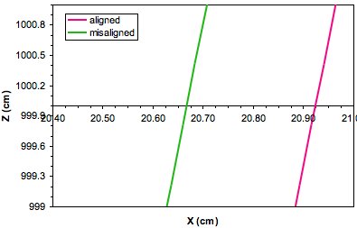
Figure 3.66: Antiproton beam trajectories for aligned (purple line) and misaligned solenoid (green line).

In Fig. 3.65 the calculated magnetic fields $B_{y}$ are shown along the z-axis at an antiproton momentum of 1.5 GeV/c. The solid line is for the misaligned solenoid and the broken line for the properly aligned solenoid. The solenoid is located in the region between $z=-170$ cm and $z=290$ cm. The dipole magnet is located in the region between $z=350$ cm and $z=600$ cm. In the solenoid region, for a properly aligned solenoid, the field $B_{y}$ is calculated to be nearly zero, while for the misaligned solenoid, $B_{y}$ has a maximum value of -69 Gauss. The dipole magnet is set to have a field integral of 0.2 Tm and it has a peak field of $\sim$1100 Gauss. The field integrals $\int{B\,dL}$ from $z=-300$ cm to 800 cm for an aligned and misaligned solenoid are shown in the bottom of the figure. For the misaligned solenoid, the field integral is $\sim$7% smaller than for the properly oriented solenoid. This results in a bending angle error of 2.6 mrad and a beam trajectory shift at $z=10$ m of $\sim$23 mm for a 1.5 GeV/c antiproton beam, as shown in Fig. 3.66. The beam bending angle errors and the trajectory shifts become smaller with increasing beam energies. For a 15 GeV/c beam, the trajectory shift is only $\sim$2.3 mm, which is shown in Fig. 3.66.

A small solenoid misalignment of 3.5 mrad in polar angle can cause a large orbit error for the solenoid. For the 1.5 GeV/c beam, the trajectory shift could be as large as 23 mm 10 m downstream of the target, while for the 15 GeV/c beam it is approximately 2.3 mm. The importance of these shifts and correction possibilities within HESR are currently discussed with the accelerator group.

3.5 Detector and Target Integration

I. Lehmann, A. Bersani, Y. Lobanov

This section describes the details of the integration of the target and all detectors inside the solenoid. We only discuss the installation of the parts which are directly attached to the magnet or in a way relevant for the design. Some of the structures are laid out only conceptually as their detailed design will not affect the overall construction of the magnet.

3.5.1 Overall Assembly Procedure

The complete magnet will be assembled in the parking position outside of the beam line. (Please refer to Fig. 2.13 of the floor plan of the hall.) As a first step the lower frame of the support structure will be assembled and mounted on the transport carriage. This will then be used to subsequently assemble the barrel part of the flux return yoke (see Sec. 3.3.5). Then the additional structures on top of the barrel will be mounted. The fully assembled cryostat will be inserted from the upstream side into the iron yoke. Only when this is done the doors of the yoke will be mounted though we have foreseen the possibility to also install or remove the cryostat with the doors in place but open. All individual parts will be aligned during the assembly but the overall alignment will be performed when the magnet is fully assembled. In order to that an optical alignment system will be used which allows to align the system with respect to the components of the ring.

As a next step the cooling lines and control lines will be connected and the solenoid will be ready for commissioning. When the commissioning will be successfully completed and the solenoid will have been approved the magnet will be powered and the central field will be mapped precisely at all operational modes.

Field mapping will be performed at this stage. Due to its almost cylindrical symmetry, the volume inside the solenoid can be measured with a fine mesh in a half-plane containing the beam axis and in several circumferences to verify the actual symmetry. The three components of the induction field will be measured, with gauges capable of a wide dynamic range, to allow a high degree of accuracy up to $2\unit{T}$ over at least 4 orders of magnitude. The field will be measured in the whole length of the yoke, up to the cryostat inner radius. Between the downward end of the cryostat and the downward door, the field will be measured up to the yoke innermost radius. The grid step will be chosen in the range $2$ to $7\unit{cm}$ according to the required accuracy and the foreseen field gradient in different regions. The field will be measured in a second stage on different circumference, around the beam axis, to measure the deviation from the perfect cylindrical symmetry. The $z$ and $r$ coordinates where to perform these measurements will be determined according to the needs of the various sub-detectors. In addition, a certain number of fixed gauges will be inserted in the muon chamber gaps in the yoke and downward door to check the consistency of the magnetic calculations.

As a very last step the muon detectors will be introduced into the gaps of the yoke, all detector systems will be installed with the foreseen support structures inside the cryostat; and finally the target system will be inserted from the top and bottom of the yoke.

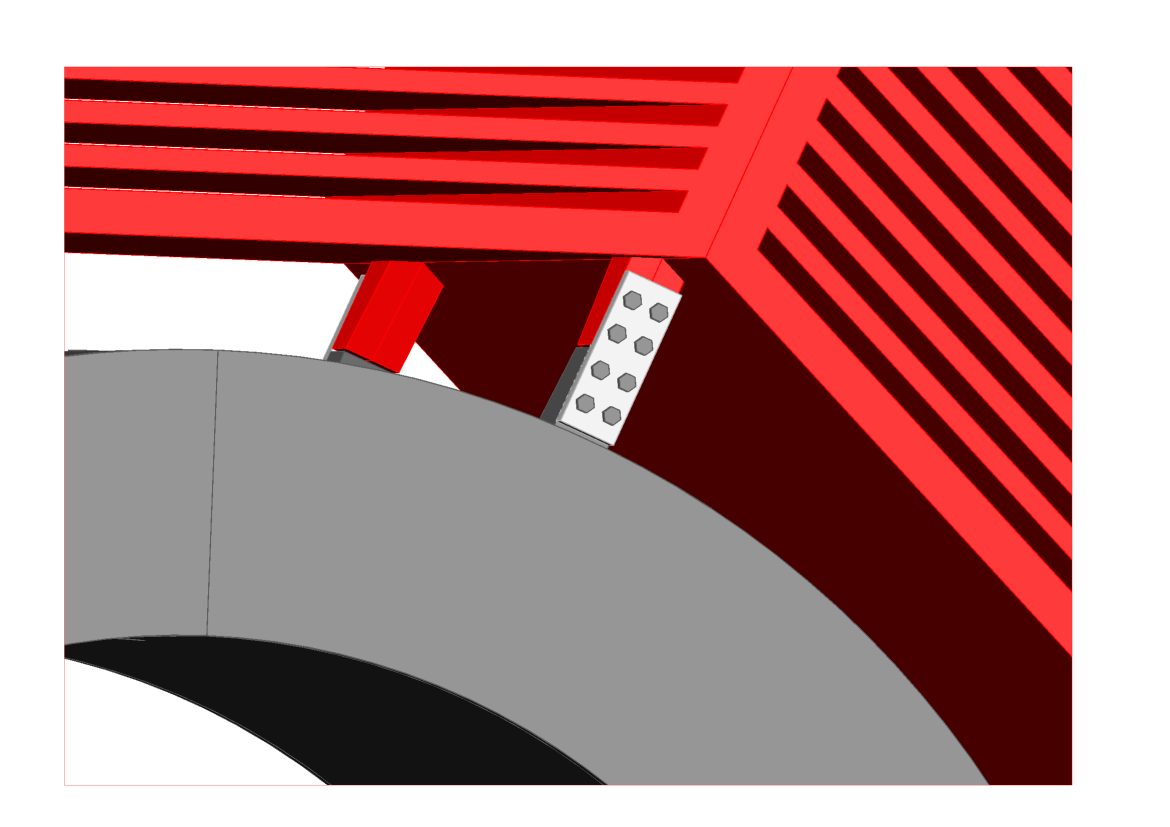
Figure 3.67: View of 2 of the 16 cryostat attachments to the flux return yoke. The attachment of the mounting points via a plate will allow for an easy adjustment of the cryostat within the barrel yoke.

3.5.2 Cryostat Mounting in the Yoke

The coil will be delivered by the manufacturer enclosed inside the cryostat with the proximity cryogenics already attached to it. Thus the cryogenic chimney, which will be located at the upstream top end of the cryostat, will be in place. The whole system will be handled as a single object. A support structure will be produced to place the whole object into the yoke barrel and allow for its safe mounting. The cryogenic chimney will be hosted in the dedicated cut out in the upper octant of the iron yoke. This structure will, most likely, be a slightly modified version of the support structure which will have been manufactured for the handling of the coil and cryostat at the company before. In principle, the same support beam and movement system could also be used to install, with minor modifications, the barrel part of the EMC in the warm bore of the cryostat.

The cryostat will be attached to the instrumented flux return yoke via 16 mounting points, 8 at each end of the cryostat. The yoke will be equipped with 16 equivalent mounting points, placed at the intersections of the beams of the octagonal barrel. The support points inside the yoke and on the cryostat will be accurately measured before the cryostat insertion, to ensure the mechanical tolerances be satisfied for safe operation. The supports will be bolted together using 8 M14 bolts each, 4 on the mounting points of the cryostat and 4 on the mounting points from the yoke. The positioning of the support structures is shown in for one of the 8 identical azimuthal positions in Fig. 3.67.

The cryostat will be bolted to the yoke and placed, using adequate spacers, to a precision better than $1\unit{mm}$ with respect to the nominal position. Further adjustments of the coil position will be possible acting on the support rods. The clearance that allows a fine position adjustment is visible where the grey and red parts meet in Fig. 3.67. The cryostat has been designed to behave as a very rigid body, as specified in the previous sections, so a deformations of the order of less than $0.2\unit{mm}$ is foreseen after the installation and the power up w.r.t.  the nominal position. This value is expected to grow no more than an additional $0.1\unit{mm}$ when the detector loads will be mounted to the cryostat.

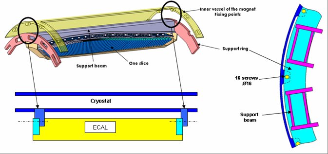
Figure 3.68: Several views detailing the attachment of the EMC barrel to the cryostat. Only a small fraction of the barrel is shown. The top left panel shows an exploded view where the brackets on the cryostat vessel and the EMC support ring are separated. The lower left and right panels show cross sections of the mounted system in the $z-y$ and $x-y$ planes, respectively.

3.5.3 Detector Installation

The detectors to be installed within the solenoid fall into two main categories: the barrel detectors brought in from the upstream side, and the forward end cap detectors brought in from the downstream side of the yoke. All detectors can be installed and removed with the magnet fully assembled but will require the doors to be open. In the following, the detectors are listed in the sequence of installation, putting emphasis on the detectors directly attached to magnet components or most crucial for the design. The weights of the individual detectors are listed in Table 2.6.

Muon Detectors

The muon detectors can be installed completely independently of the other detectors. The single detector element will be an array of $8$ Mini Drift Tubes, of variable length according to the position where the element should be installed. A cross section of an array of MDT is shown in Fig. 3.69. The elements can be inserted individually, simply by hands being relatively light ($\sim 1\unit{kg}$ per linear metre of array).

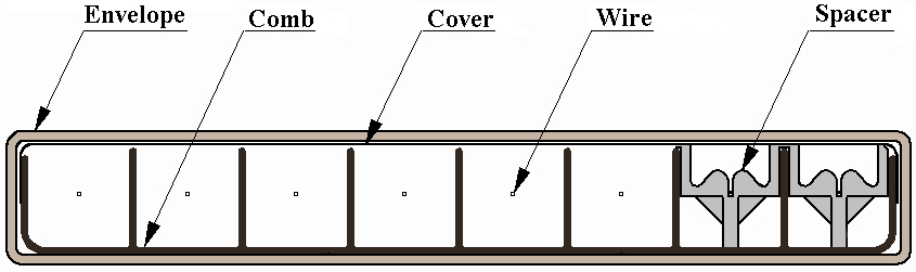
Figure 3.69: Cross section of a muon MDT module.

The detectors installed in the iron yoke will be slid in the proper clearances from downstream, with the end doors open. Shorter elements are foreseen in the upper octant, due to the target recess. The cables will be routed through the slits present in the barrel corners, at downstream end. To ensure a proper cabling scheme, the muon detectors will be the first system to be install to the yoke.

The detectors installed in the downstream doors will be inserted in their clearances from the sides. Different lengths are foreseen to allow the best coverage of the octagonal surface of the doors. The cables will be routed from the sides of the end doors.

Barrel EMC

The Barrel Electromagnetic Calorimeter (EMC) will be connected to the inner surface of the cryostat using 32 dedicated mounting brackets at the inner rim of the cryostat vessel. The attachment between the EMC and the cryostat is shown schematically in Fig. 3.68. The design ensures that the fully assembled barrel of the EMC can be moved in from the upstream side after the installation of the cryostat inside the flux return yoke (see Fig. 3.70). The weight of the Barrel EMC is estimated to be about $20\unit{t}$, which will be by far the major contribution to the load that must be sustained by the cryostat from the detector side. The cryostat itself has been designed to take into account this additional load with adequate safety margins. For further details about EMC design and installation procedures, please refer to EMC TDR [PANDA:TDR:EMC].

Figure 3.70: Artistic view showing the mounting procedure of the Barrel EMC. After the assembly of all parts in a self-supporting barrel structure outside of the solenoid the whole system will be transferred on a central beam into the operation position. After attaching the structure to the cryostat the inner beam and support crosses are removed to make space for the inner detector installation.

Barrel DIRC

The Cherenkov detector based on detection of internally reflected Cherenkov light covering the large angles (Barrel DIRC) will be mounted into the solenoid in 2 independent parts. First the barrel of quartz slaps will be inserted into the solenoid just inside the Barrel EMC. Its weight of 300 kg will be supported by the common support system for the inner detectors which is attached to the cryostat.

The ring structure, where read-out boxes with a weight of about 800 kg are encased, will be mounted separately. It will be mounted after the inner detectors (see next section) will be in place. It is attached to the upstream end of the Barrel yoke by a spider-like structure supported using the same kind of mount points as in the downstream end.

Figure 3.71: Forward end cap of the EMC and Disc DIRC with mounting brackets which will also serve the purpose of guiding the cables and supplies to the cut outs in the iron yoke.

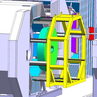
Figure 3.72: Artistic view of the mounting procedure for the forward end cap of the EMC showing the frame which allows the safe movement of the system into the flux return yoke. Some additional support structures have been omitted for visibility.

Inner Detectors and Beam Pipe

The beam pipe and the interaction cross will be installed with the micro-vertex detector (MVD) and the outer tracker, in a single support frame. The pipe with the frame will be prepared outside the yoke, then the detectors will be mounted on it and it will be placed in its working position from the upstream side. It will travel on a dedicated rail system attached to the lateral surface of the cryostat.

Turbo pumps will be installed to remove the background gas coming from the target just outside both the upstream and downstream ends of the solenoid magnet. The locations of the pumps are given in Table 2.4.

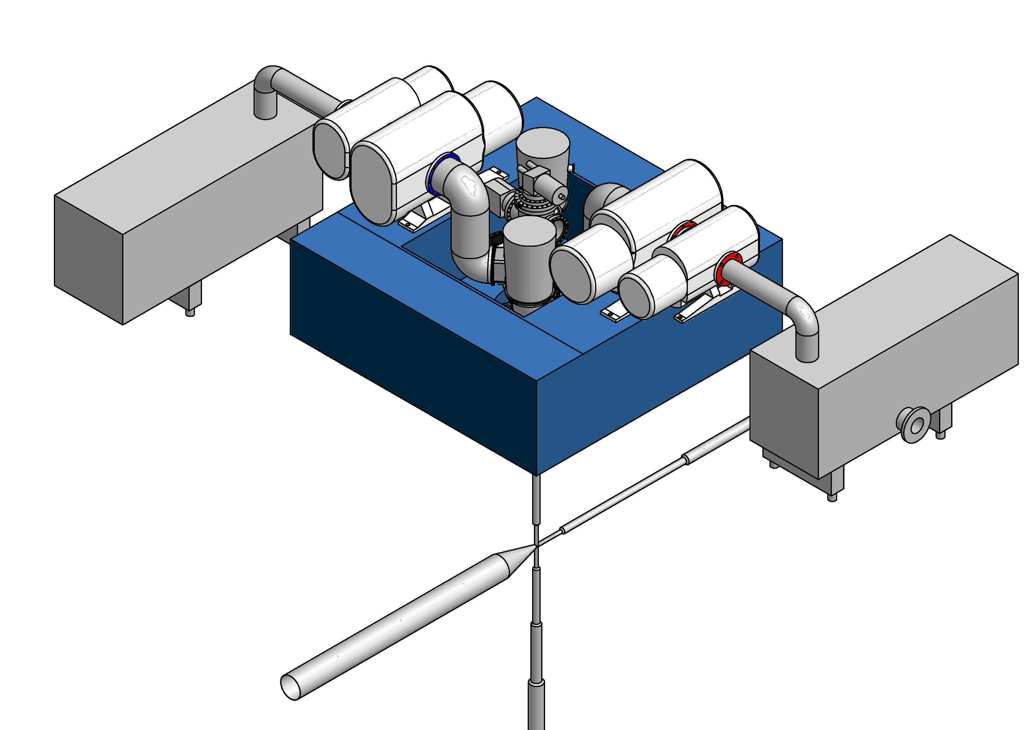
[Bird’s eye view] [Cross section viewed from upstream]

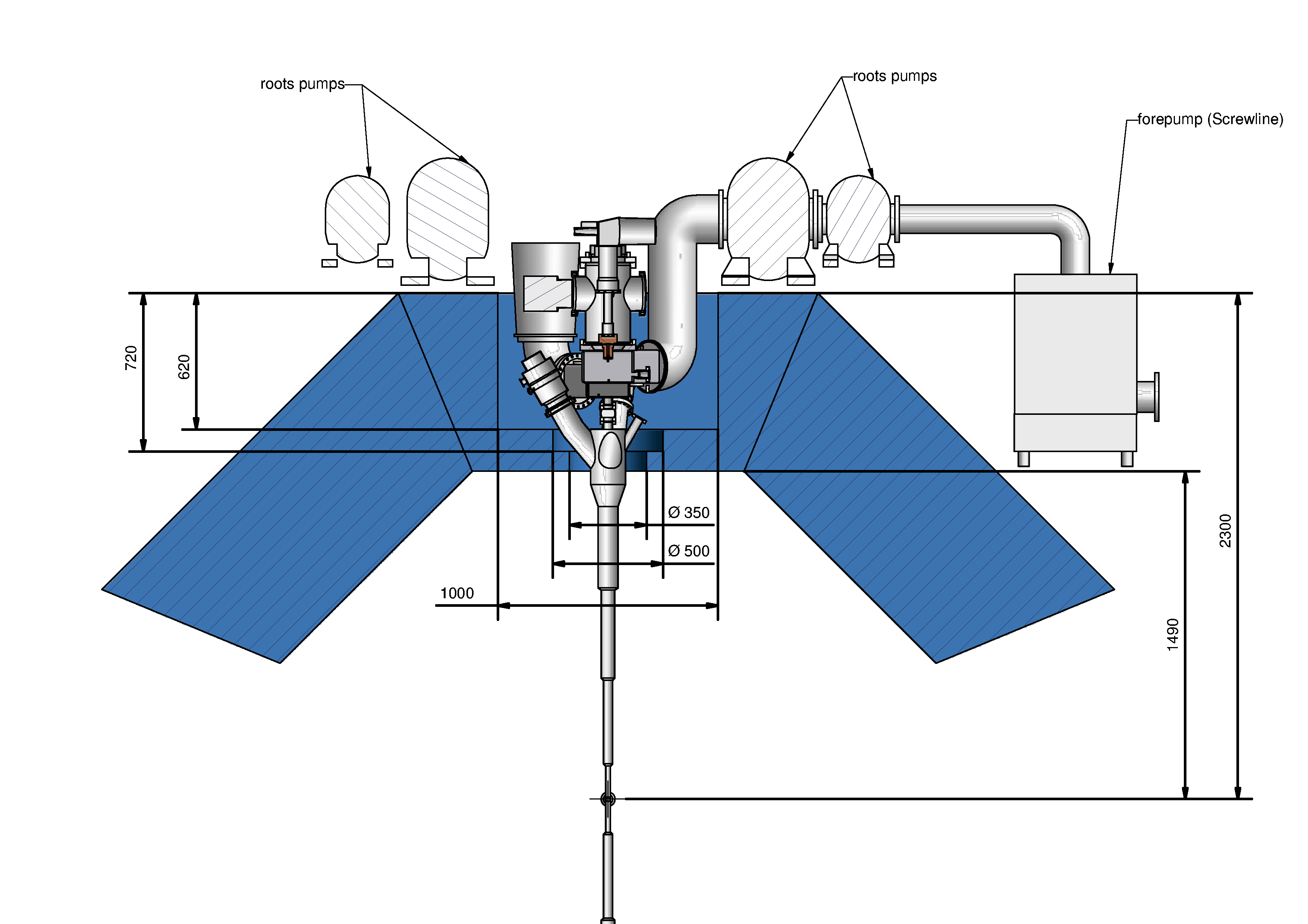
Figure 3.73: Views of the foreseen integration of the generator of the cluster-jet target in the yoke of the solenoid.

Forward End Cap Detectors

The three stations of Gas Electron Multiplier (GEM) detectors will be mounted as the first item inserted from the downstream end of the solenoid. The details of their attachment are not yet specified precisely. It is envisaged that the comparably small weight of these detectors will be attached to the same frame which holds the inner detectors.

The Disc shaped DIRC detector in the forward end cap will be mounted just in front of the forward end cap of the EMC. Mechanically it will be assembled onto the same holding structure and installed together with the EMC. The Forward end cap of the EMC is shown in Fig. 3.71. Here the DIRC is mounted and covers the crystals of the EMC. Once the DIRC is attached the whole system will be placed on a temporary frame which will allow to safely move the array to the operational position and mount it to the inner surface of the yoke (see Fig. 3.72).

3.5.4 Target Integration

The installation of the target production and recovery stages will take place after the beam pipe cross with the detectors has been inserted. The upper and lower straight sections of the target pipe will be inserted from the top and bottom of the flux return yoke, respectively. The connection inside the solenoid will be done through fast joints which can be operated from a distance.

A recess in the upper octant of the barrel is needed to host the turbo-molecular pumps and cryogenics for the production stage, as the cluster jet target requires to keep a maximum distance of $2\unit{m}$ between the nozzle and the interaction point for safe operation.

The roughing pumps will be installed on the sides of the production stage, as close as possible to the turbo-molecular pumps, on dedicated supports. Views showing the integration of the production stage in the instrumented flux return yoke are given in Fig. 3.73. The recovery stage will be attached to lower part of the target pipe in a similar way. For that a smaller recess of 500 mm depth and a diameter of 1 m is sufficient.

The target dump will be installed under the yoke barrel. A proper clearance under the support structure is foreseen to allow the vacuum chamber and pumping installation: in addition, a platform suspended to the yoke carriage is foreseen to allow the hosting of the fore-vacuum pumps and of the proximity electronics of the dump itself.

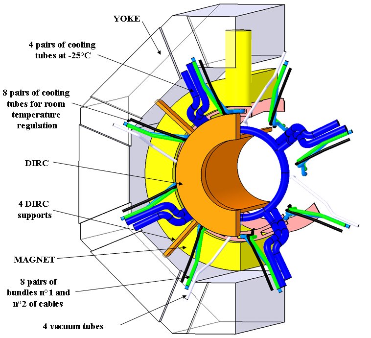
Figure 3.74: Schematic view showing the routing of the cooling pipes (blue) and all other supply lines and signal cables of the Barrel EMC at the upstream end of the solenoid. For visibility details have been omitted and magnet and detectors are cut in half.

3.5.5 Cable and Supply Routing

Cables and pipes coming from the detectors will be guided to the outside of the yoke in their majority through 16 cut outs in the corners of the instrumented flux return barrel, 8 at the upstream and 8 at the downstream end of the barrel, $42\unit{cm}$ wide and $14\unit{cm}$ long. (Please also refer to Sec. 3.3.2 and Fig. 3.21.)

Together with the supply lines, all signal cables coming from most of the detectors will be routed through these slits. It should be emphasised that all cables will be mounted taking into account additional magnetic and Laplace forces acting on them. The upstream end cap of the EMC and the central inner and outer trackers will have their supply lines and signal cables guided to the upstream end close to the beam pipe. As this will not affect the magnet design this is detailed elsewhere. The routing of the Barrel EMC supply lines and signal cables through the upstream end of the yoke is illustrated schematically in Fig. 3.74.

Chapter 4 Forward Spectrometer

I. Lehmann, J. Lühning, E. Lisowski

The central solenoid will be augmented by a large-aperture dipole with 2 Tm bending power. It will be equipped with drift chambers for particle tracking and scintillation counters for time-of-flight measurements inside the aperture, and followed by a full forward detection system. The Forward Spectrometer (FS) will cover angles of up to 5 and 10 degrees in the vertical and horizontal planes, respectively. A view of part of the system showing the instrumented dipole is shown in Fig. 4.1.

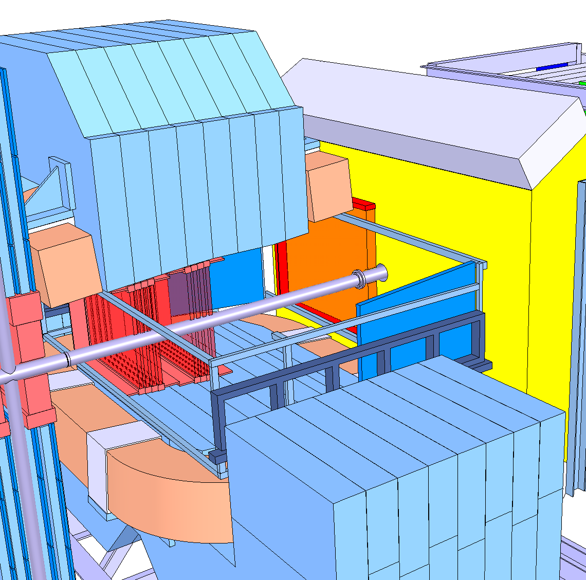
Figure 4.1: View of the dipole magnet cut for visibility and parts of the forward detectors of PANDA.

The major challenge in the construction of the dipole is the achievement of a 2 Tm field integral over a short longitudinal extent, while maintaining reasonable operational costs. The length of the dipole along the beam axis determines the position of the forward detectors. However, the area of the forward detectors obviously increases quadratically with distance to the interaction point. Thus it is necessary to minimise the dimensions of the dipole in this direction. On the other hand, a shorter dipole with large aperture requires higher fields which increase the saturation of the iron yoke. Saturation increases the required currents through the coils considerably. The use of a superconducting coil, although superficially attractive, proved impractical and uneconomic for several reasons discussed in the following. Another important feature of the dipole will be that it will need to be part of the accelerator lattice of the High Energy Storage Ring (). Ramping capabilities compatible with the accelerator will be ensured by segmenting the yoke and providing an appropriate power supply. Extensive optimisation studies have led to a detailed design, which is described later in this chapter.

4.1 Conceptual Design

The conceptual design of the dipole magnet was detailed by a collaboration of research groups experienced in the design and construction of such magnets. The main contributors were engineers from JINR, Dubna, physicists and engineers from GSI, Darmstadt, and physicists from the University of Glasgow. The design studies addressed the issues of physics requirements, as laid out above, field quality, mechanical considerations and economic construction and operation. The option to shield the beam from the field by an iron plate was considered but it proved unacceptable. The primary reason not to further consider this option was the required acceptance for zero degree particles. Furthermore, large background contributions were expected if placing large amounts of material close to the beam. In Fig. 4.2 two options for the coil design are shown which were considered but finally dismissed.

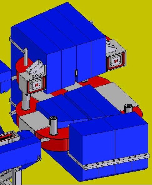
[Superconducting design] [Bedstead-type coil design]

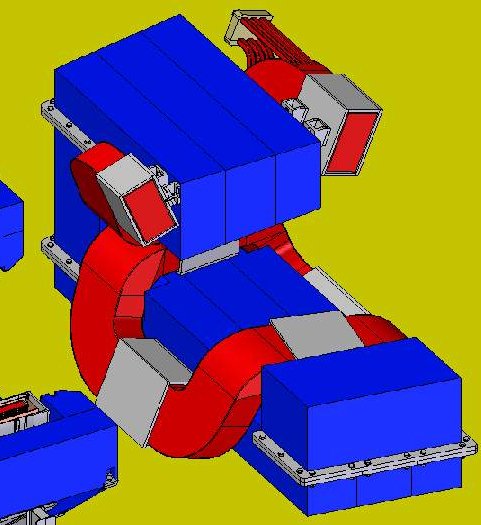
Figure 4.2: Examples for design options considered for the dipole magnet. (a) Superconducting coils decrease the power consumption in the cable but impose mechanical constraints and require refrigeration. (b) A non-planar coil (shown here is the bedstead type) may allow a rather short design but the field properties are less convenient than in the planar construction which was finally chosen.

A design selection has now been made, based on the reasoning and criteria presented below. Minor changes may however be introduced when the details of the construction are evaluated together with the manufacturer. A superconducting coil does not provide an attractive alternative because of the following points.

• The vertical force on each coil will be higher than 100 tons. For a superconducting coil this would demand great skill in the design of the suspensions. Apart from the imposed risks and costs this would require a considerable amount of cryogenic cooling, which would marginalise savings due to reduced power consumption.

• A suspension ensuring low heat losses would require rods in the yoke gap, which would reduce the acceptance of the detectors.

• Our design foresees racetrack shaped coils. The reason for this is a good magnetic stiffness not only on the beam axis but also at an horizontal deflection angle of $10^{\circ}$. A disadvantage of non-circular coils is the fact that they are subject to bending moments in the winding plane. For the large cross sections of normal-conducting coils this poses no problem; but superconducting coils with their rather small cross sections would need additional bending stiffness in the winding plane.

• The dipole magnet will be part of the lattice and therefore needs to be ramped during acceleration within 60 s. This requirement imposes high demands on the conductor and its cooling for a superconducting dipole. Special measures would have to be taken to limit coupling and eddy current loss [Wilson:1983] and to ensure cryogenic stability.

• The construction cost for a dipole magnet with superconducting coils is significantly higher than using resistive coils. From rough estimates we have deduced factor of 2 higher construction costs for a similar superconducting dipole magnet.

• The operation of a superconducting magnet is more challenging and higher efforts on maintenance and survey are required than in the case of resistive coils. Finally, the risk of downtimes or failure of operation is minimal in the latter case.

In conclusion, we have taken the decision to pursue the resistive coil option. Similar considerations have led to the design choice of other large aperture dipole magnets (see e.g. the LHCb magnet [LHCb]).

The optimum coil shape has been determined based on studies of current, effective field, stray field and geometrical dimensions. Many different layouts have been considered, including bedstead and deck-chair shapes. Finally it was found that racetrack type coils, i.e. laid out in one plane, provide satisfactory performance and lowest cost simultaneously.

The effect of field clamping has been studied in detail. It was shown that, indeed, field clamping is required to separate the fields from the solenoid and dipole magnets. It was found that it is advantageous to extend the upstream field clamp such that it can simultaneously act as an extension to the range system for the muon identification above $5^{\circ}$ and $10^{\circ}$ in vertical and horizontal angles, respectively. This system will replace this field clamp fully, but will be mechanically independent and will be mounted only after the installation of all detectors. Therefore, we treat it as a separate part in Sec. 4.4.1. To the downstream side of the dipole the necessity of field clamping is not yet clear, as the details of the detectors in that region are not yet defined. We foresee the possibility to attach several sheets of iron downstream of the coils. Details of their design are not crucial to the design of the remaining components of the magnet.

4.2 Coil and Yoke Design

I. Lehmann, J. Lühning

The total length along the beam has been optimised to balance magnet and detector requirements. A longer magnet would have lower power dissipation, however the area the forward detectors have to cover would increase quadratically with increasing distance from the interaction point. The solution was to select a magnet length of 2.5 meters, which achieves the desired field integral without considerable saturation in the iron yoke. The overall height and width are 3.9 and 5.3 metres, respectively.

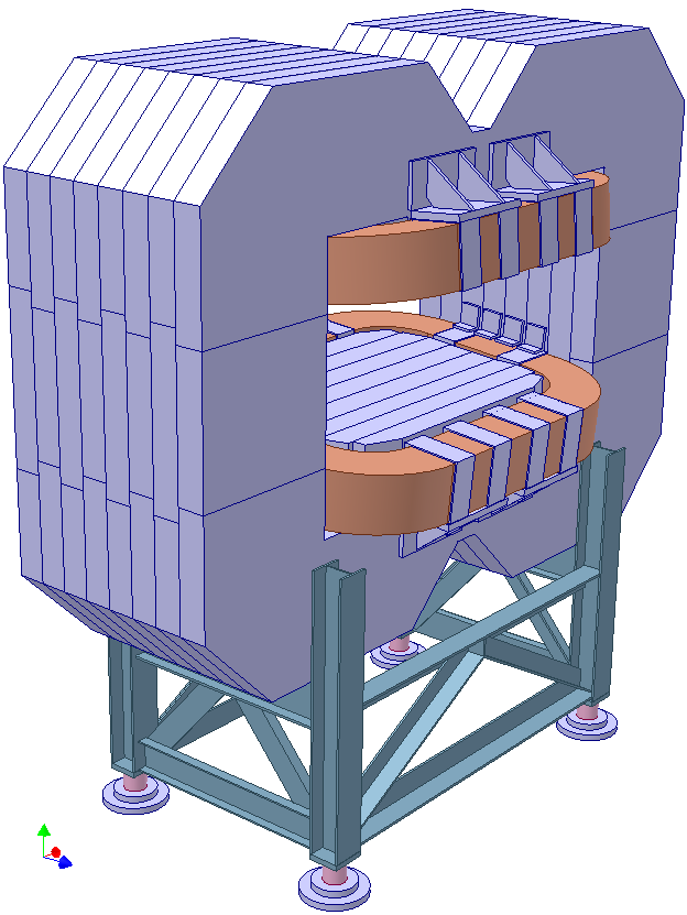
Figure 4.3: View of the large-aperture dipole magnet from the downstream side.

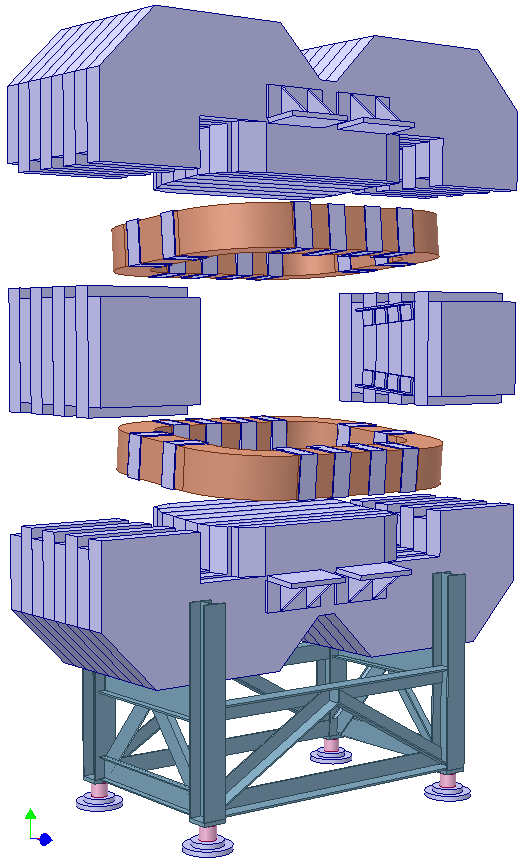
Figure 4.4: Exploded view of the flux return yoke from the downstream side.

The yoke is to be built out of plates of low carbon steel. We foresee AISI 1006 here, which is a high quality, low carbon (0.06%) magnetic steel. The flux return yoke will be segmented for two reasons. First of all a moderate segmentation is mandatory as the magnet needs to be ramped with the acceleration of particles in HESR. At the anticipated ramp time of 60 s and a plate thickness of 20 cm the eddy currents will stay below 5 A/cm², the power dissipation below 400 W, and the delay between the current and field will be less than two seconds (see Sec. 4.3.4). Secondly, the weight of each individual magnet part is below 15 t and so the crane in the experimental area can carry each part. Hence there is no need for an additional crane for assembly. The total assembled weight will be of the order of 220 t. An exploded view showing the mounting points for the coils is shown in Fig. 4.4. Three projections in the three coordinate planes are shown in Figs. 4.5 to 4.7, respectively.

Figure 4.5: Side projection of the dipole magnet showing the overall length and minimal gap in millimetres. The beam comes in from the left. Please note that the opening angle of the coils given here does not fall on the $\pm 5^{\circ}$ line from the interaction point.

Figure 4.6: Top projection of the dipole magnet showing the dimensions of the yoke in millimetres. The beam comes in from the top.

Figure 4.7: Projection from the downstream side of the dipole magnet showing the dimensions of the yoke, the gap opening and the distance to the HESR floor in millimetres.

Figure 4.8: Schematic view of the coil arrangement in the dipole magnet. The upper and lower coils are inclined in the $z-y$ plane by plus and minus $5^{\circ}$, respectively. The $z$ axis is defined by the antiproton beam trajectory before the entrance into the magnetic field of the dipole magnet and the $y$ axis is the vertical direction.

The opening of the yoke and its coils are designed such that particles emitted from the target with vertical angles below $5^{\circ}$ in the vertical plane traverse the magnet fully and reach the detectors in the forward region. As the mounting structure and the frames of the in-gap detectors (see Sec. 4.4) use some of the space, the rectangular upper and lower coils are located 5.5 cm outside the upper and lower $5^{\circ}$ planes (see Fig. 4.8). The use of inclined coils rather than horizontal coils reduces the forces on the muon filter by a factor of 3 and reduces the power consumption. The pole shoes will be manufactured such that the frame has the appropriate space while keeping the iron of the flux return closing in as far as possible to reach a maximum field integral. In addition the surfaces will be kept without steps in order to keep field gradients minimal. A tentative sketch of the envisaged design in shown in Fig. 4.9. The yoke aperture opens out from 0.80 m to 1.01 m in vertical direction while staying constant at 3.1 m in the horizontal plane. The constant horizontal aperture width will facilitate the installation of tracking and time-of-flight detectors to distinguish slower particles that do not exit the magnet.

Figure 4.9: Sketch of the pole shoe geometry in the $z-y$ plane. This shape allows the accommodation of in-gap detectors without constraining the vertical acceptance while keeping the field maximal and continuous.

Copper is the selected conductor material, despite being slightly more expensive than aluminium, due to its lower resistivity and better ductility. Only with copper the required small bending radius can be achieved. Copper can cope with higher current densities and reduces operational costs due to a 37% reduction in power dissipation. It is calculated that the increased purchase cost due to the selection of copper rather than aluminium will be fully compensated by the reduced power consumption costs in less than one year of operation. Additionally, the choice of a copper conductor allows a more compact magnet design, thereby reducing the cost for the forward detectors. The selected hollow copper conductor has a $30\times 24\,$mm² cross section and a cooling channel diameter of 10 mm. A likely arrangement would be to have 6 double pancakes with $14+14$ windings each in both the upper and lower coils. The main parameters of the magnet are listed in Table 4.1.

Item	Value
Coils
Type	Resistive
Material	Copper
Weight	$\sim 18$ t
Arrangement	Race track, inc. $\pm 5^{\circ}$
Conductor diam.	$30\times 24\,$mm2
Water cooling	Channel $\varnothing=10$ mm
Conductor current	2.16 kA
Current density	3.38 A/mm2
Total current	727 kA
Single turn length	8.68 m
Mean resistivity	18.5 n$\Omega$ m
Total dissipated power	360 kW
Inductance (incl. yoke)	0.87 H
Stored energy	2.03 MJ
Flux Return Yoke
Material	Steel XC06
Lamination	$\sim 20$ cm
Weight	$\sim 200$ t
Dim. ($H\times W\times D$)	$3.88\times 5.3\times 1.64$ m3
Gap opening ($H\times W$)	$0.80-1.01\times 3.10$ m2

Table 4.1: Overview of the main parameters of the dipole magnet. The depth $D$ denotes the length along the beam direction $z$ axis.

We assume that the 24 pancakes will be fed by cooling lines in a parallel arrangement, where the water inlet and outlet are located on the inner and on the outer sides of the winding, respectively. Then we would require 3.9 l/s of water and the temperature difference between inlet and outlet would be 22 K. The water velocity in the cooling channels of 10 mm would reach about 2 m/s and the pressure drop would be 8 bar.

To ensure a proper operation of the dipole magnet, a slow control system will be built which provides the interface to HESR and diagnostic systems. The following magnet systems will be monitored

• Interface to . This system will guarantee that the control and diagnostic systems of exchange information and are fully synchronised with all systems of the dipole. The precise layout is not yet defined.

• Current control will be used to monitor the magnetic field intensity and the stability of the dipole magnet.

• Temperature control. The temperature of the copper coils will be monitored by several temperature sensors located at different positions on the upper and lower coils.

• Magnetic field control. Two Nuclear Magnetic Resonance (NMR) probes and 5–10 Hall probes in critical places are foreseen to be used to directly measure the magnetic field intensity and stability.

• Cooling water flow control. The flow of cooling water will be controlled by water flow meters at several locations.

The chief tasks of the diagnostic system are listed in the following.

1. Process signals fast to generate alarm and interlock signals for magnet safety in emergency situations.

2. Record control parameters in the normal operation regime and provide data logging.

3. Allow remote control of all parameters, in particular the full integration within the control systems. Display the data at the operator’s console.

4. Process signals to generate control responses to optimise the magnet operation.

The magnet and auxiliary equipment control system will incorporate a distributed computer control system composed of commercially available components. Detailed design of the slow control system will be performed starting from 2010.

The field mapping will be performed using existing equipment at GSI and with the help of the GSI Magnet Technology Group. It is envisaged that for each of 5 different current settings one full 3D field map would be determined with a grid size of 7, 5 and 2 cm in $x,y$ and $z$, respectively. This work will be performed as soon as the magnet is fully commissioned and 60 days are estimated for the measurements. Interpolating between the grid points and maps would allow us to determine the magnetic field at every point in the spectrometer opening and any current to sufficiently high accuracy.

The magnet design has been optimised and is finalised to a high level of detail. A few minor modifications to the design might, however, be imposed by constraints or recommendations from the manufacturer during the tendering process.

4.3 Performance

I. Lehmann, J. Lühning

4.3.1 Structural Considerations

The studies of the mechanical stability have concentrated on the coils and the stand of the dipole magnet. The bulk mass of the yoke is stemming from the rigidly connected steel plates which provide a good stability by themselves.

Figure 4.10: Deformation of one half of the upper dipole coil, enlarged by 1000 times for visibility. The winding is supported at the vertical upstream and downstream surfaces of the dipole yoke. The loose bearing is in the region between the pole shoe and the flux return part of the yoke. The colours show the Von Mises stresses (red indicates stresses of about 100 MPa, light blue 10 MPa and dark blue below 10 MPa).

Finite Element Model (FEM) calculations were performed with the Generative Structural Analysis module of CATIA [mag:CATIA]. Out of symmetry reasons it is sufficient to analyse only one half of one coil. The result of this calculation is shown in Fig. 4.10. The force input for this model was taken from a calculation using TOSCA [mag:TOSCA_2008]. The total Lorentz force of one coil will be about 110 t in vertical direction while its weight will be only about 10 t. It is difficult to represent the orthotropic properties of the winding precisely. For our calculation, however, a coarse approximation of the properties is sufficient. This was done by introducing 4 empty channels along the perimeter of the winding such that the winding is stiffer in longitudinal direction than in the transverse directions. The support rings holding the winding are assumed to consist of aluminium. Between the support ring and the winding we assume a 5 mm thick layer of soft material (Young’s modulus 4 GPa) in order to avoid high local stresses. A soft material was also applied for the loose bearing in the centre of the magnet. As visible in Fig. 4.10 those calculations reveal that the stresses in the windings stay well below 10 MPa while the stresses in the support stay below 120 MPa. These results show that we have kept a good safety margin in the design of the coils.

Figure 4.11: Deformation of the dipole support structure in the extreme case of a strong seismic load exactly at the very moment where the magnet is suspended only by two legs during the alignment procedure (see text).

The support structure for the large aperture dipole magnet has been designed to safely support the weight of the magnet and additional installations even under exceptional situations. Two extreme cases have been considered in detail:

1. a horizontal acceleration of 1.5 m/s²,

2. the whole weight resting on only 2 diagonally opposite legs of the support structure.

In the very rare occasion of strong seismic activity case 1 may occur. Case 2 may occur during the alignment procedure of the dipole, when one leg is pushed up or released further than the two neighbouring legs (e.g. with the help of a hydraulic jack). The worst case scenario would be if a seismic activity would lead to a horizontal acceleration in the direction diagonal to the two supporting legs precisely in the very moment where the whole load is suspended only by two legs. Though this is extremely unlikely, this case has been studied (see Fig. 4.11). The maximum stress does not exceed 180 MPa, i.e. 3/4 of the elastic limit of ordinary structural steel. Thus, even in this unlikely event the structure would guarantee the mechanical safety of the dipole magnet.

4.3.2 Static Field Properties

The major objective for the field is to achieve a field integral of 2 Tm at 15 for particles emitted from the interaction area below horizontal and vertical angles of $10^{\circ}$ and $5^{\circ}$, respectively. These particles will escape the Target Spectrometer and reach the Forward Spectrometer, where the large-aperture dipole magnet together with the tracking devices will enable the momentum reconstruction of charged particles. Most crucial are the highest momentum particles, as their bending is smallest. Particles with momenta of more than a factor of 15 below the beam momentum will be deflected so much that they will not transverse the full magnet and hence experience a smaller field integral. This poses, however, no problem as the momentum is reconstructed very precisely also with a reduced field integral, because these particles are bend much stronger.

[Contour plot of $B_{y}$ in the $z-y$ plane at $x=0$. The linear scale starts at 0.80 T (blue) and ends at 1.05 T (lilac).] [View from the downstream side showing the field in a colour map from 0.5 T (blue) to 1 T (lilac) in the $y-x$ plane at $z=4.75\,$m.]

Figure 4.12: Vertical magnetic field component $B_{y}$ in the opening of the dipole magnet in two different views.

Figure 4.13: Dipole field for several straight trajectories in the horizontal plane of the dipole. The tracks originate at the interaction point with angles respective to the beam direction of $0^{\circ}$ (red solid curve), $7^{\circ}$ (blue dashed curve) and $10^{\circ}$ (black dotted curve).

Figure 4.14: Bending angle of tracks with $P=P_{beam}$ through the magnetic field of the dipole using ray-trace calculations. The bending varies by 10%, but this can be easily handled by the PANDA track reconstruction.

The magnet was designed such that the field between the pole shoes stays as uniform as possible for a magnet with such a large aperture (about $1\times 3\,$m). Field calculations have been performed with a full 3D model of the magnet using TOSCA [mag:TOSCA_2008]. Figs. 4.12 show views of the field in $z-y$ and $y-x$ planes at $x=0$ and $z=4.75\,$m, respectively. One observes that the field in the central region is constant within 20% while it falls off steeply close to the coil location. Here the change along the particle path is unimportant compared to any change within the $x-y$ plane, as the latter influences the field integral experienced by the particle. In Fig. 4.13 the actual field seen by particles transversing the magnet under three different trajectories is shown. The relevant quantity for the momentum reconstruction is, however, the bending of the tracks due to the passage through the magnetic field. Assuming particles with beam momentum the change of angle induced by the magnetic field has been studied in ray-trace calculations. Particles with lower momenta will be bend more than that and hence can be reconstructed better. The resulting differences of a mean bending angle of $2.2^{\circ}$ are in the order of 10% at the very corners of the yoke gap (see Fig. 4.14).

Figure 4.15: Detail of the field in the region between the end-cap of the solenoid and the entrance of the dipole magnet. This view corresponds to an $z-y$ slice several centimetres off the axis ($x=0$).

These differences are easily handled by the track reconstruction software provided that the actual field is known to the appropriate detail. Therefore the magnet is designed such that the field remains a smooth function in space over the whole volume where particles are tracked.

In Fig. 4.15 the combined field of the dipole and solenoid shows how the intermediate muon filter in front of the dipole will act as an effective field clamp and will help to separate the two spectrometers magnetically and reduce stray fields.

The field strength between the pole shoes of the magnet will not follow the current in the coils in an absolutely linear way. One effect is saturation of the iron which limits the maximum flux and hence changes the resulting field. This effect is static and will start to significantly influence the field at about half of the full current. The saturation will occur mainly at the edges of the pole shoes (see Fig. 4.16). Thus the actual bending power of the magnet will be about 2.02 Tm at full current, while with half the current 1.05 Tm will be reached. This effect of the saturation can be illustrated by calculating the bending power and inductance normalised by the fraction of the full current (see also blue lines in Figs. 4.18). The $\int{B\,dl}$ and the current density in the coils is listed in Table 4.2 for 10 beam momenta. At full current, the total energy is 2.03 MJ, the total inductance is 0.87 Henry.

Figure 4.16: Magnetic field strength $H$ in the flux return of the dipole at full current. The colour scale is logarithmic. Only one upper quarter of the magnet is shown as the other quarters show identical distributions. The field strength is clearly reaching maximal values at the edge of the pole shoes, while it stays two orders of magnitude lower in the bulk of the flux return yoke.

$p_{\mathrm{beam}}$	$T_{\mathrm{beam}}$	$\int{B\,dl}$	Total Current
$[$GeV/c$]$	$[$GeV$]$	$[$Tm$]$	$[$A$]$
1.5	0.83101	0.2	69144
3.0	2.20503	0.4	138298
4.5	3.65850	0.6	207480
6.0	5.13465	0.8	276821
7.5	6.62019	1.0	346557
9.0	8.11050	1.2	416917
10.5	9.60357	1.4	488486
12.0	11.09835	1.6	562660
13.5	12.59429	1.8	641346
15.0	14.09104	2.0	726962

Table 4.2: Dipole parameters for 10 antiproton beam momenta $p_{\mathrm{beam}}$ ranging between 1.5 and 15 GeV/c. Listed are the corresponding kinetic energy $T_{\mathrm{beam}}$, the integral of the field along the $z$ axis $\int{B\,dl}$ and the total current in the coils.

Figure 4.17: Stray fields downstream of the dipole magnet. Shown is half of the upper downstream field clamp of the dipole and a representative volume where the read out of a potential RICH detector would be located. The maximum field in this volume would be 25 Gauss.

4.3.3 Stray Fields

The detectors downstream of the dipole will be affected by stray fields, in particular some detectors which have read-out systems sensitive to magnetic fields. As their design is not yet defined in detail, definite limits for the field strength are not finally set. We have, however, enough flexibility to control the fields in that region by adding field clamps downstream of the coils. As an exemplary scenario we have calculated the field for the most crucial system. The closest detector with possibly field sensitive read-out is the RICH detector. We have studied the field at the location of its likely read-out, though this detector is not yet fully designed. The outcome is illustrated in Fig. 4.17. The use of a field clamp with 3 layers of iron with 4 cm thickness each will result in stray fields below 25 Gauss at the location of a possible RICH readout. This calculation does not include possible additional shieldings at the location of the read out. All other detection systems are either located much further away or foresee field insensitive read-out systems.

4.3.4 Dynamic Properties

The dipole will form part of the accelerator lattice deflecting the beam and hence needs to be ramped for every cycle in a synchronised fashion with the other bending magnets in the . This dynamical change of currents in the coils and subsequent change of field strength induces eddy currents in the flux return yoke. These counteract the magnetisation and demagnetisation at ramp-up and ramp-down, respectively. Thus the field changes slower than the current does. The effect will be decreased by the lamination but still needs to be compensated in order to guarantee beam stability over the full ramp.

[Bending power] [Inductance]

Figure 4.18: Normalised bending power (a) and inductance (b) versus current in the coils of the dipole magnet. Shown are two cases: in blue the magnet is ramped very slowly such that eddy losses can be neglected, while the red curves indicate the situation in the fast ramping foreseen at , i.e. in 1 minute from 25% to full nominal current.

Figure 4.19: Envisaged start of the ramp procedure. A smooth transition is reached by increasing the sweep rate linearly from 0 to 1.25% over a period of 2 s.

Figure 4.20: View of half of the dipole magnet indicating the density of the eddy currents 12 seconds after the start of the ramp – colour coding from 0 (dark blue) to the maximum value of 4 A/cm² (pink).

The time foreseen to accelerate antiprotons from injection momentum (3.8 GeV/c) to full momentum (15 GeV/c) in the is 60 seconds. Thus it is required to change the current in the coils with a rate of 1.25% of the nominal dipole current per second. The ramp-up procedure is envisaged as following. Before injection the magnet is ramped to 25% of the nominal current $I_{\mathrm{nom}}$. At this plateau the current is kept constant for a short while, which allows the (re)injection of antiprotons. Meanwhile the eddy currents will drop. For our calculations we assume now the following sequence. The ramp-up is started by a parabolic current increase over 2 s. This avoids discontinuities in $dI/dt$ which may harm the power supplies. Hence, the actual current $I=I_{\mathrm{nom}}\left[\frac{I_{\mathrm{inj}}}{I_{\mathrm{nom}}}+p_{0}\,t^{2}\right]\,,$ where $t$ is the time in seconds, and the current at injection $I_{\mathrm{inj}}=0.25\,I_{\mathrm{nom}}$. Setting the parameter of the polynomial $p_{0}$ to $2.6\times 10^{-3}\,\mathrm{s}^{-2}$ guarantees a moderate delay, such that the system reaches a steady ramping speed of $dI/dt=0.0125\,I_{\mathrm{nom}}/\mathrm{s}$ after 2 s. The power supply would need to provide additional 25 V to compensate the resistance due to induction if considering a nominal current of 2.1 kA in the coils. Please also refer to Fig. 4.19.

In this scenario with the moderate lamination of 20 cm the eddy currents induced in the dipole yoke reduce the inductance and the bending power only by less than 2% (see Fig. 4.18). The total power losses due to the eddy currents will stay below 400 W during the whole ramp time. In Fig. 4.20 one half of the yoke is shown indicating the density of the eddy currents.

4.3.5 Influence on HESR Beam

In order to quantitatively understand the orbit errors caused by the spectrometer, 3D Tosca magnetic field calculations are carried out. For the dipole the major source of uncertainty is the non uniform saturation in the yoke iron as it is ramped with the beam momentum. 10 different excitation currents corresponding to 10 different antiproton beam energies are used for the dipole, which are shown in Table 4.3. The excitation currents are selected such that the different energy antiproton beams have the same bending angle.

$p_{\mathrm{beam}}$	$\int{B\,dl}$		Relative
	nom.	model	deviation
$[$GeV/c$]$	$[$Tm$]$	$[$Tm$]$
1.5	0.2	0.200000	$+4.2850\times 10^{-7}$
3.0	0.4	0.400000	$+1.9000\times 10^{-7}$
4.5	0.6	0.600001	$+1.5333\times 10^{-6}$
6.0	0.8	0.800006	$+7.8725\times 10^{-6}$
7.5	1.0	1.000019	$+1.9074\times 10^{-5}$
9.0	1.2	1.200045	$+3.7556\times 10^{-5}$
10.5	1.4	1.399972	$-2.0050\times 10^{-5}$
12.0	1.6	1.600052	$+3.2750\times 10^{-5}$
13.5	1.8	1.800047	$+2.6321\times 10^{-5}$
15.0	2.0	1.999948	$-2.6110\times 10^{-5}$

Table 4.3: Dipole parameters for 10 antiproton beam momenta $p_{\mathrm{beam}}$ ranging between 1.5 and 15 GeV/c as in Table 4.2. Here the nominal integral of the field along the $z$ axis $\int{B\,dl}$ is compared to calculations using a realistic model in TOSCA (nom. and model, respectively). The relative deviations stay at a level of $10^{-5}$ or below.

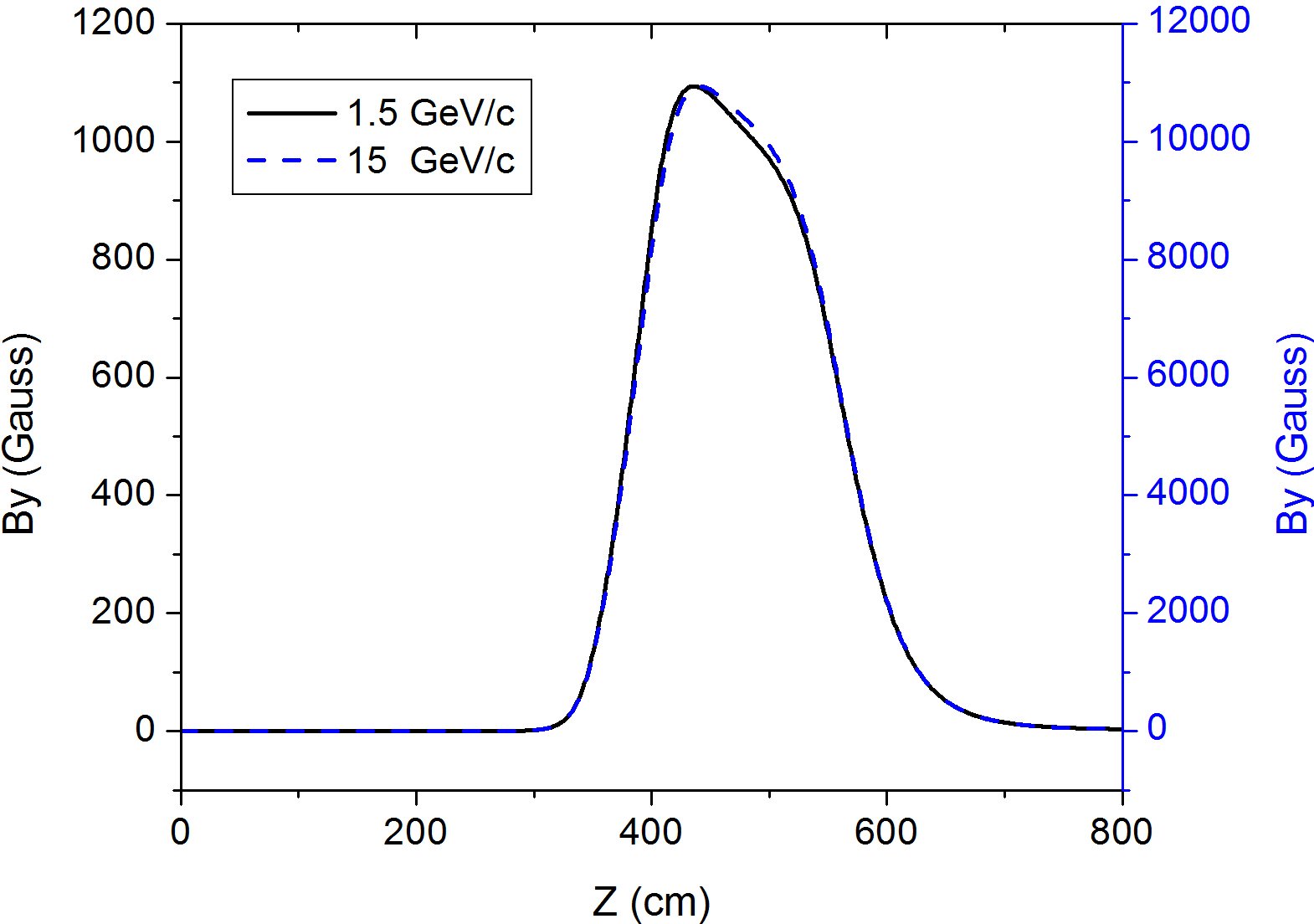
Figure 4.21: Field distribution along the central line for different dipole settings for a 1.5 GeV/c (solid black line and left scale) and a 15 GeV/c beam (dashed blue line and right scale).

In Fig. 4.21, the dipole magnetic fields along the z axis are shown. The dashed line is for the 15 GeV/c antiproton beam, and the solid line is for the 1.5 GeV/c antiproton beam. To compare the differences in the field distributions, the scale for the 1.5 GeV/c antiproton beam is a factor of 10 larger than the one for the 15 GeV/c beam. It is observed that the field changes slightly its shape when scaling between those extremes.

As mentioned in the previous paragraph, the field distribution differences arise from a consideration of non uniform saturation in the iron. The dipole will have a field integral of 2 Tm. The maximum peak field in the dipole mid plane is around 1.1 T, while the maximum magnetic field in the iron pole shoe is as high as 2.9 T, which appears at one of the corners. The magnetic field distribution through the pole shoes will be not uniform and in addition the iron saturation will be non uniform. The saturation itself will not affect the field distribution too much, but the influence of the non uniform saturation will be more serious. To reduce the non uniform saturation effect, a chamfered or rounded pole shoe could be used.

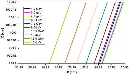
Figure 4.22: Beam trajectories of antiproton beam of momentum from 15 to 1.5 GeV/c. the leftmost side on is for a 15 GeV/c beam, while on the rightmost site is that for a 3 GeV/c beam. The blue line is the trajectory for the 1.5 GeV/c beam.

In Fig. 4.22, beam trajectories of antiproton beams in a range of momenta from 1.5 to 15 GeV/c are shown. These calculations assume a perfectly aligned solenoid. On the leftmost side is the trajectory for a 15 GeV/c beam, while on the rightmost site is that for a 3 GeV/c beam. The distance between these two trajectories at $z=10$ m is around $0.4$ mm. The other trajectories are located in between these two extremes, and except for the 1.5 GeV/c beam, a beam trajectory is normally located on the left side of a beam trajectory having a smaller energy. The blue line is the trajectory for the 1.5 GeV/c beam. The distance between the 3 GeV/c beam trajectory and the 1.5 GeV/c beam trajectory at $z=10$ m is around 0.03 mm. It should be pointed out that the field errors from the TOSCA simulation (see Table 4.3) also contribute to the orbit shift shown in Fig. 4.22, and has the largest effect on the beam trajectory of the 1.5 GeV/c beam. Other beams will also suffer from the same effect, but the orbit variations are much smaller.

In summary the non uniform saturation effect in the dipole magnet will also introduces a small trajectory shift which can be as large as 0.4 mm. This could be reduced by using chamfered or rounded pole shoes. But since this is a minor contribution, it is not clear yet if this will be necessary.

4.4 Detector Integration

E. Lisowski, J. Smyrski

The construction of supports for the Forward Spectrometer detectors is closely connected with the design of the dipole magnet, since the supports must be integrated in the yoke, to avoid any reduction of the aperture of the magnet, leading to limitations of the angular and momentum acceptance of the system. Besides, the detector supports will be mounted directly on the magnet yoke in order to reach high reproducibility of the detectors position with respect to the magnetic field. This is of special importance for the drift chambers, which reconstruct the momentum of charged particles on the basis of deflection of their trajectories in the dipole magnetic field.

The Forward Spectrometer will be equipped with three pairs of tracking drift detectors, hence six independently operating detectors, each containing four double-layers of straw tubes. The first pair of drift detectors (DC1, DC2) will be mounted in front of the dipole magnet, the third (DC5, DC6) further downstream, behind the magnet. The second pair (DC3, DC4) will be installed inside the magnet gap in order to track low momentum particles hitting the magnet yoke inside the gap. The drift detectors in each pair will be mounted on a common support frame. This solution allows to reach a high accuracy of relative positioning of the detectors – better than 0.1 mm. It also eases the installation of the detectors in the experimental position.

High mechanical precision of the mounting elements, used to fix the support frames on the magnet yoke, will allow to reach a high reproducibility of the detector position with respect to the magnet yoke, when dismounting the detector themselves for servicing and mounting them again on the magnet. The frames will be rigid enough to hold the weight of the detectors, which is evaluated to be about 50 kg for the smallest one – DC1 – and about 400 kg for the largest one – DC6. The frame construction will also guarantee high stability of the drift detector positions with respect to the magnet – on the level of 0.05 mm – during periods of data taking.

The detector components of the Forward Spectrometer foreseen for the particle identification (the RICH detector, the TOF wall, the forward muon detectors) and for the calorimetry (the electromagnetic calorimeter) as well as the luminosity monitor will be mounted on a common platform. The platform will be used to support the detectors on a proper height with respect to the beam line. The total mass of the detectors is about 60 tonnes. The platform will be equipped with a driving system allowing to move the detectors between the experimental area and the parking position. The driving system should guarantee a reproducibility of the detector positions with respect to the magnet yoke better than 1 mm.

In the four following subsections we describe respectively:

• the construction of supports for mounting detectors between the solenoid and dipole magnet;

• the construction of support frame for detectors inside the magnet gap;

• the design of supports for mounting the drift detectors at the exit of the dipole magnet;

• the design of the movable platform for the Forward Spectrometer detectors.

The presented design of the detector supports was worked out by the groups from the Cracow University of Technology (CUT) and from the Jagiellonian University (JU), in close cooperation with the whole collaboration.

4.4.1 Detectors Between Solenoid and Dipole

Drift Chambers DC1 and DC2

The first pair of drift detectors (DC1, DC2) will be installed in the space between the Target Spectrometer downstream door and the yoke of the dipole magnet. The chambers will be mounted on the cross formed by the beam pipe and a vertical pipe used for pumping (see Fig. 4.23). After that the detectors will be connected together by means of steel joints and the vacuum pipe will be attached to the detector frames by means of two clamps. The connection between the detectors will guarantee the required high reproducibility of the relative positioning.

During the installation of the drift detectors, the TS downstream door will be opened. The detectors will be mounted on the dipole magnet yoke by means of vertical steel profiles attached to the horizontal coil holders (see Fig. 4.23). After that the segment of the beam pipe passing through the DC1-DC2 pair will be connected to the TS beam pipe with proper flange connection. This connection is located inside the TS downstream door opening. The following step will be the insertion of the frame which will hold the detectors inside the dipole gap (see next section). This will be rolled in from downstream direction and the beam pipe will be connected with a flange foreseen at the $z$-position of the dipole magnet coils. The access to this connection will be limited by the coils to about 70 cm in the vertical direction and to 60 cm in the horizontal direction by the remaining free space between the chambers DC2 and DC3. This space will be sufficient for humans to access the beam pipe and connect the flanges safely.

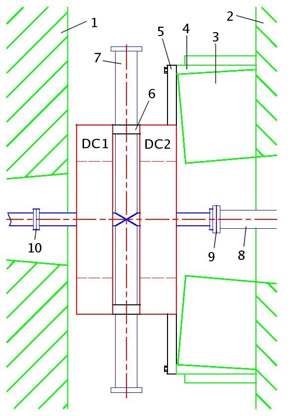
Figure 4.23: Pair of drift detectors DC1 and DC2 mounted on the yoke of the dipole magnet: 1 – TS forward door, 2 – yoke of the dipole magnet, 3 – coil, 4 – coil holder, 5 – steel profile for hanging the detectors, 6 – connecting element, 7 – vacuum pipe, 8 – beam pipe, 9,10 – beam pipe connections.

Muon Filter

Surrounding the vacuum pipe and the tracking detectors DC1 and DC2, a removable muon filter will be placed which serves as a continuation of the muon detectors in the downstream door for the high momentum part of the muon spectrum.

The filter will consist of five layers of 6cm thick iron interleaved with the same drift tube detectors used within the laminated solenoid yoke. It is segmented in four individual blocks (upper-right, upper-left, lower-right, lower-left). The four segments will have cut-outs to respect the enclosed detectors and equipments and can be removed easily as blocks by crane to give access to the drift chambers and the beam and vacuum pipes.

The iron of the muon filter, in addition, will decouple the magnetic fields of the solenoid and the dipole and reduces the stray field of the dipole in the region between the two magnets.

4.4.2 Yoke Gap Fittings

Support Frame

The design of the frame foreseen for supporting detectors between the poles of the dipole magnet is shown in Fig. 4.24. The frame will be made of standard closed stainless-steel profiles. It will have a trapezoidal shape fitting the aperture of the magnet and will be supported by two rails mounted on the side walls of the magnet gap. The rails will be used for sliding the frame in the gap during the installation. The frame is foreseen to support the drift detectors DC3 and DC4 as well as two TOF side walls. It will be also used for supporting a 3 m long part of the beam pipe crossing the magnet gap.

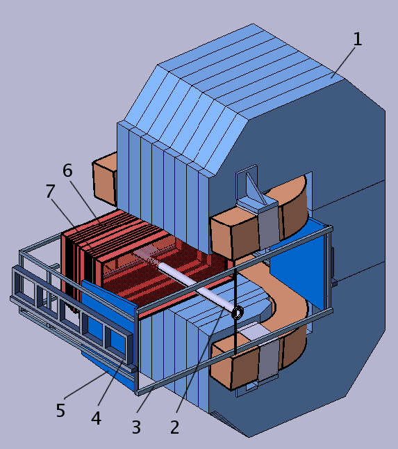
Figure 4.24: Support frame for detectors inside the dipole magnet gap: 1 – magnet yoke, 2 – beam pipe, 3 – movable frame, 4 – rails mounted on the wall of magnet, 5 – time of flight detector, 6 – DC3, 7 – DC4.

Detector Installation

The installation of detectors in the frame will be done with the frame rolled out of the magnet gap. The positions of the drift detectors with respect to the frame will be fixed with the precision better than 0.1 mm by means of reference pins. The beam pipe will be inserted in the central openings in the detectors and subsequently it will be hanged on the frame by means of two vertical bars. Afterwards, the detectors will be cabled and connected to supply lines. The installation of the whole assembly inside the gap of the dipole magnet will be accomplished just by rolling it inside the gap. Excesses foreseen in the guidance of the detector cables and the supply lines should allow for a free movement of the structure during the installation. The movement of the frame inside the magnet gap will be limited by mechanical blockade. Positioning pins mounted on the blockade system are used to fix precisely the position of the support frame with respect to the magnet yoke.

4.4.3 Drift Chambers at the Exit of the Dipole

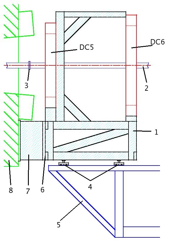
Figure 4.25: Side view of the support frame for the drift detectors DC5 and DC6: 1 – support frame, 2 – beam pipe, 3 – beam pipe connection, 4 – adjustable feet, 5 – forward platform, 6 – connection between support frame and cantilever, 7 – steel cantilever, 8 – dipole magnet yoke.

[] []

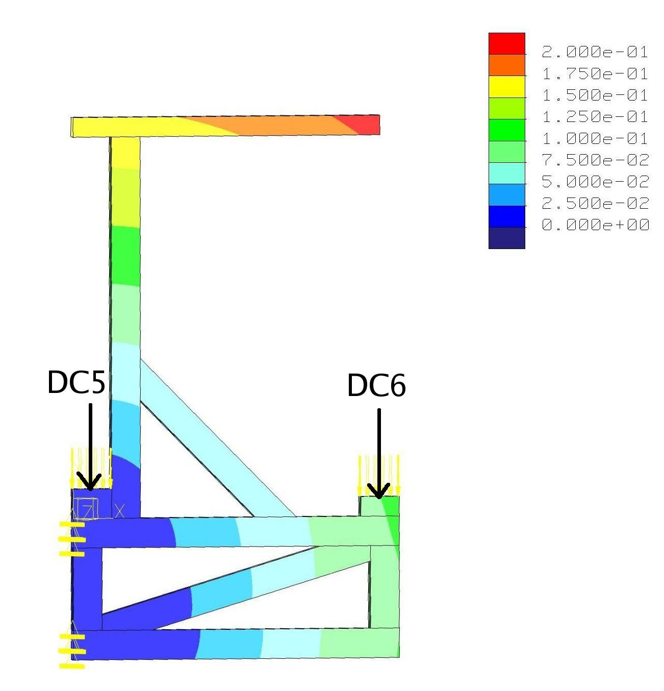
Figure 4.26: a) Von Mises stresses in MPa and b) deformation in mm of the support frame due to weight of DC5 (300 kg) and DC6 (400 kg).

The support for the third pair of drift chambers, DC5 and DC6, will be built as a frame with a rectangular box shape with attached bracket to hold them in proper orientation and position (see Fig. 4.25). The support will be constructed using standard stainless steel profiles. For the total weight of the chambers pair, about 700 kg, a profile with transverse dimensions of 50 mm x 150 mm and wall thickness of 4 mm will guarantee sufficient stiffness of the support. A side view of the support frame is shown in Fig. 4.25. In the service area, the frame will stand on four feet on the platform for the forward detectors. After installation of the drift detectors, the frame will be transferred on the platform to the experimental area and it will be hanged on two steel cantilevers that will be permanently fixed to the dipole magnet yoke. To assure reproducibility of the frame position with respect to the yoke, precisely machined junctions between the frame and the cantilevers are foreseen. After mounting the frame on the cantilevers, the frame feet can be released, since the load is taken over by the cantilevers.

The stresses in the frame under the expected load of DC5 (300 kg) and DC6 (400 kg) lie in a safe range below 7 MPa (see Fig. 4.26). The maximum deformation of the frame is equal to 0.2 mm (see Fig. 4.26) and is acceptable from the point of view of the required positioning reproducibility.

4.4.4 Platform for Forward Detectors

Construction

The components of the Forward Spectrometer detection system including the RICH detector, the TOF-wall, the electromagnetic calorimeter and the forward muon detectors, as well as the luminosity monitor, will be placed on a common platform which will be used to support them on a proper height with respect to the beam line. It will also allow to move the detectors from the experimental area to the service position. A view of the proposed platform is shown in Fig. 4.27.

The area of the platform will be 6.70 m x 4.05 m and the height will be 2.14 m. The heaviest detectors, the electromagnetic calorimeter (8 tonnes), and the forward muon detectors (49 tonnes), will be set up in the central part of the platform. The RICH detector and the forward TOF-wall, with a total mass of about 2 tonnes, will be placed near the dipole magnet on a lowered part of the platform. The platform will be $\sim 0.5\unit{m}$ lower in the upstream segment to host the RICH detector. The lowered part of the platform will be also used to support the drift detectors DC5 and DC6 during the transfer between the service position and the experimental area. The far end of the platform in downstream direction will be used for supporting the luminosity monitor.

The platform will be built as a framework based on two carrying beams with attached wheel sets. In the footing, below the floor level, reinforcing beams with attached wheel tracks will be placed.

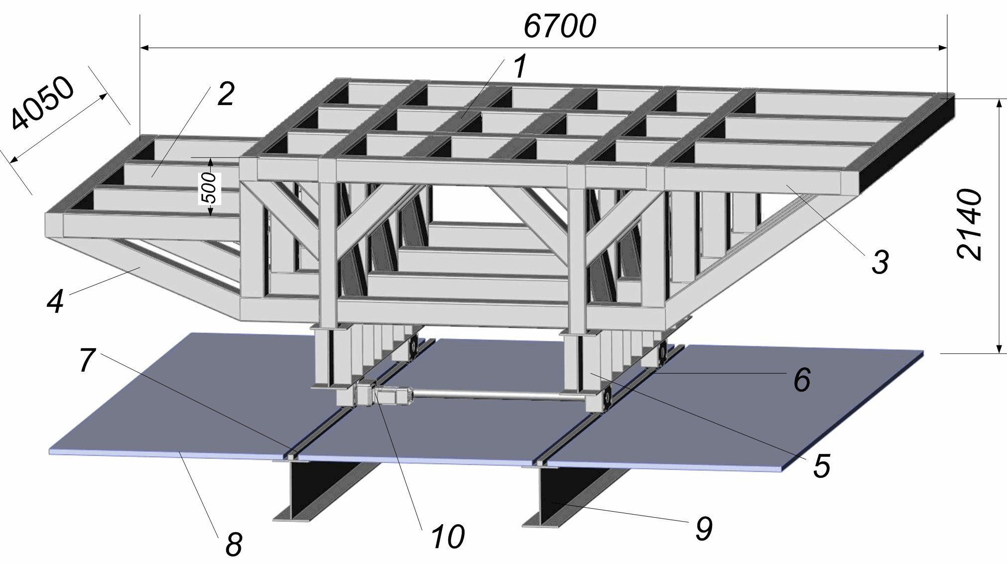
Figure 4.27: Model of the platform for the forward detectors: 1 – main platform, 2 – lowered part of platform, 3,4 – framework made of closed profiles, 5 – carrying beams, 6 – wheel sets, 7 – wheel tracks, 8 – plate determining the floor level, 9 – reinforcing beams, 10 – driving unit.

To build the carrying beams we will use a construction profile commonly used in the industry according to the standard EN 10024. The profile will be additionally strengthened by vertical ribs. The same type of profile will be also used to build the reinforcing beams. The platform framework will be built of rectangular steel profiles (material: S355J2, according to EN-10025-2). The total mass of the platform is 5.5 tonnes.

Driving system

For the driving system of the detector platform, we plan to use wheels with two rims moving on rectangular bars welded to rails. The chosen wheel diameter is 250 mm and the spacing of wheel rims is by $2s=1$ mm larger than the width of the rail bars equal to $k=110$ mm. Wheels will be mounted in blocks which will be fastened under the carrying beams (Fig. 4.27). To move the platform, with its total foreseen load of 60 tonnes, four wheel blocks will be sufficient. The platform will be driven by a single electric motor, with transmission shaft transferring the torque to two wheels. Movement of the platform with maximum velocity of 0.05 m/s can be realised by an electric motor with the power of 0.5 kW. The electric motor will be equipped with a gear box and a brake and will be steered using an electronic system of movement control.

Stress calculations

Calculations of mechanical stress in the platform were carried out using the application Pro/Engineer - Pro/Mechanica. Under the expected load of 60 tonnes, the maximum stress will be lower than 75 MPa (see Fig. 4.28) and is acceptable for the used material. Fig. 4.28 presents corresponding displacement contours. The maximum displacement will not exceed 0.5 mm and thus is acceptable from the point of view of the required positioning accuracy of the detectors.

[] []

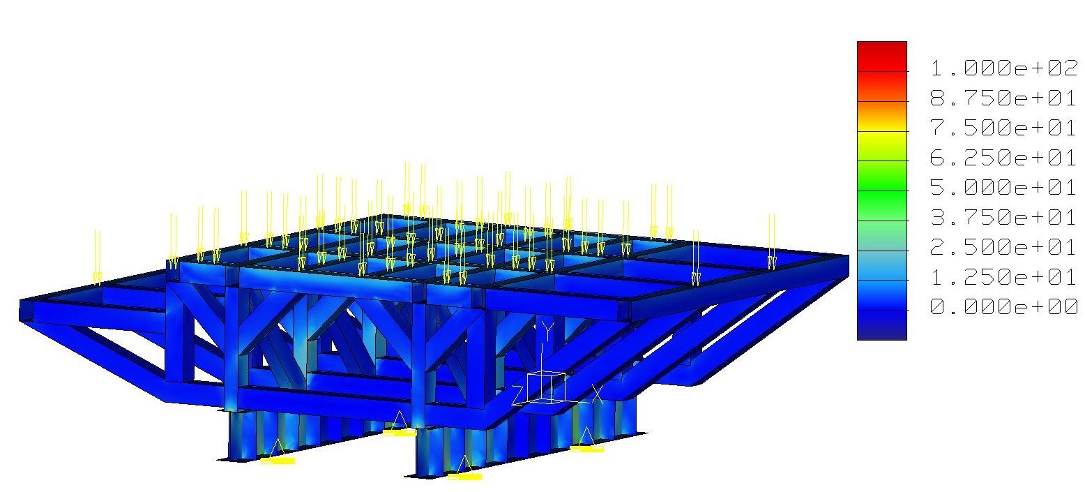
Figure 4.28: a) Von Mises stresses in MPa and b) deformation in mm of the platform due to load of 60 tonnes.

Transport to FAIR

For transfer from manufacturer site to FAIR, the platform it will be divided into three subunits: central platform and two side platforms. The dimensions of these subunits allow for delivery of each of them by conventional means of transport: trucks or railway. After transport to FAIR - to the PANDA experimental hall - the three subunits will be assembled by means of screwing and welding.

Chapter 5 Organisation

I. Lehmann

The two large spectrometer magnets will be built by seven groups from universities and research institutes in Germany, Italy, Russia, Poland and the UK. The institutions and their abbreviations are listed in Table 5.1.

Abr.	Institution
CUT	Cracow University of Technology,
	Kraków, Poland
FZJ	Forschungszentrum Jülich,
	Jülich, Germany
Gla	University of Glasgow,
	Glasgow, United Kingdom
GSI	GSI Helmholtzzentrum für
	Schwerionenforschung GmbH,
	Darmstadt, Germany
INFN	INFN, Sezione di Genova,
	Genova, Italy
JINR	Joint Institute for Nuclear Research,
	Dubna, Russia
UJ	Jagiellonian University,
	Kraków, Poland

Table 5.1: Table of abbreviations and institutions responsible for the design and construction of the magnets at .

5.1 Work Packages and Responsibilities

Five distinct primary work packages have been identified. These comprise the design and construction of the following items.

1. The coil and cryostat of the Target Spectrometer. The overall responsibility is taken by INFN, Genoa.

2. The flux return yoke of the Target Spectrometer, which will serve simultaneously as multi-layer absorber for a large-angle muon detection system. The overall responsibility is taken by JINR, Dubna.

3. The large-aperture dipole magnet for the Forward Spectrometer. The overall responsibility is taken by the University of Glasgow.

4. The support structures and detector mountings for all of the Forward Spectrometer. The overall responsibility is taken jointly by the Jagiellonian University, Kraków and the Cracow University of Technology.

5. The railing systems and movement of the whole Target Spectrometer and the platform with the Forward Spectrometer detectors. The overall responsibility is taken jointly by GSI, Darmstadt and Cracow University of Technology.

The Forschungszentrum Jülich takes care of the spectrometers’ integration into the HESR, which is particularly important for the dipole, since it will be part of the accelerator/storage ring lattice.

The responsibility for the detector mountings inside the Target Spectrometer will remain with the individual detector groups, while the magnet group will provide only mounting points. A detailed list of work packages has been worked out, and responsibilities have been identified, which have been approved by all groups. These are listed in Table 5.2, where the responsible institutions are listed by their abbreviations specified in Table 5.1. Where responsibilities are shared the main responsible is given first and the secondary is indicated in brackets. The main responsible institution will always supervise the work package and take responsibility for a timely and full completion.

Task		Responsible
Instrumented Flux Return
	Design, documentation, tender, supervision of construction	JINR
	Material procurement, manufacturing, assembly and transport preparation	JINR
	Assembly and tests at company	JINR
	Transport to FAIR	JINR
	Interface for muon system	JINR
Coil & Cryostat
	Cold mass cooling circuit design	INFN
	Selection of cable	INFN
	Mandrel and winding (spacers, connectors…) design	INFN
	Mechanical suspension of the cold mass in the cryostat	INFN
	Design of intermediate temperature shields	INFN
	Feed lines and turret	INFN(FZJ)
	Coil Protection system	INFN
	Coil diagnostic and DAQ	INFN(GSI)
	Tender and procurement	INFN
	Follow-up of the cable procurement & tests	INFN
	Follow-up of the coil construction	INFN
	Follow-up of the cryostat construction	INFN
	Follow-up of the cryogenic turret feed lines	INFN
	Coil, cryostat, turret final assembly at manufacturer site	INFN
	Cryogenic and electric tests at company	INFN
	Transport to FAIR	INFN
Dipole Magnet
	Final dipole design	Gla
	Procurement and quality assurance (no assembly)	Gla
	Dipole slow control	Gla
Detector Support Structures
	Platform for the FS detectors	CUT
	Supports in the dipole magnet gap	CUT
	Wire chamber supports of the FS	UJ
	Absorber system for muon filtering between TS and FS	CUT
Magnet Support Structures
	Rail system and moving of solenoid	GSI(CUT)
	Solenoid support structure	JINR
	Dipole support structure	Gla
Assembly and Commissioning at FAIR
	Assembly of yoke and support structures	JINR
	Installation of cryostat and supply lines	INFN (JINR)
	Assembly of dipole magnet and power supply	Gla
	Alignment of magnets	GSI (FZJ)
	Commissioning of solenoid	INFN (JINR)
	Commissioning of dipole	Gla
	Field mapping for both magnets	GSI
	Assembly of detector supports in the FS	CUT(UJ)

Table 5.2: Table of work packages listing the individual work packages and the responsible institutions by the abbreviations as listed in Table 5.1. The institutions listed in brackets are responsible for a specific part of the WP but the overall responsibility is taken by the leading institution.

5.2 Timelines

The timelines are driven by the envisaged start of commissioning of HESR in 2014. In particular, the Forward Spectrometer needs to be in place in order to allow any beam operation, as the dipole forms part of the accelerator lattice. In order to allow for field mapping, detector installation and commissioning the magnets and support structures must be in place and commissioned by 2013.

5.3 General Safety Aspects

The design details and construction of the magnets including the infrastructure for operation will be done according to the safety requirements of FAIR and the European and German safety regulations.

All electrical equipment will comply to the legally required safety code and concur to standards for large scientific installations following guidelines worked out at CERN to ensure the protection of all personnel working at or close to the components of the experimental facility. Power supplies will be mounted safely and independently from large mechanical loads. Hazardous voltage supplies and lines will be marked visibly and protected from damage by any equipment which may cause forces to act on them. All supplies will be protected against overcurrent and overvoltage and have appropriate safety circuits and fuses against short cuts. All cabling and connections will use non-flammable halogen-free materials according to up-to-date standards and will be dimensioned with proper safety margins to prevent overheating. A safe ground scheme will be employed throughout all electrical installations of the experiment. Smoke detectors will be mounted in all appropriate locations. The more specific safety considerations are discussed in the respective sections throughout the document.

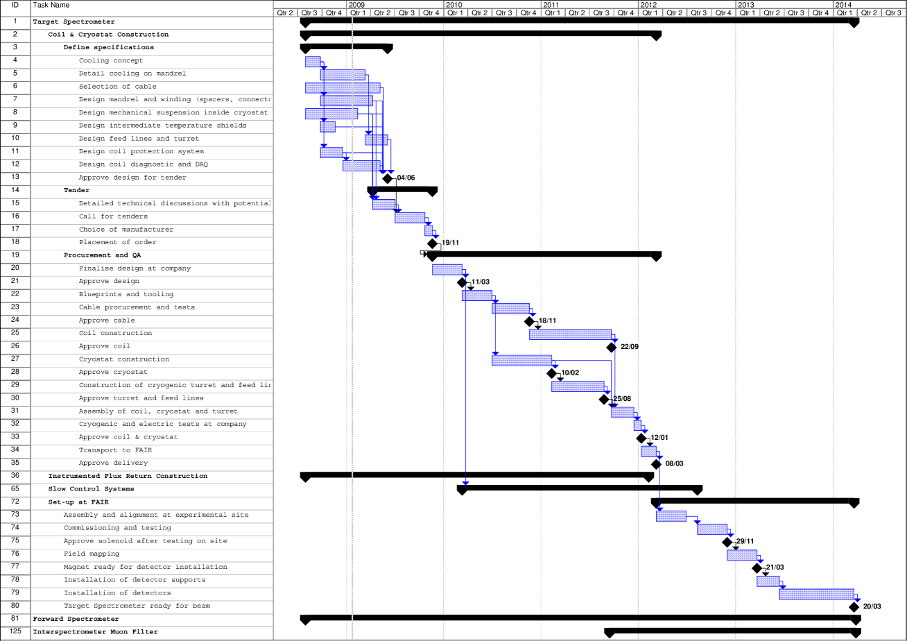
Figure 5.1: Timelines highlighting the coil and cryostat of the Target Spectrometer.

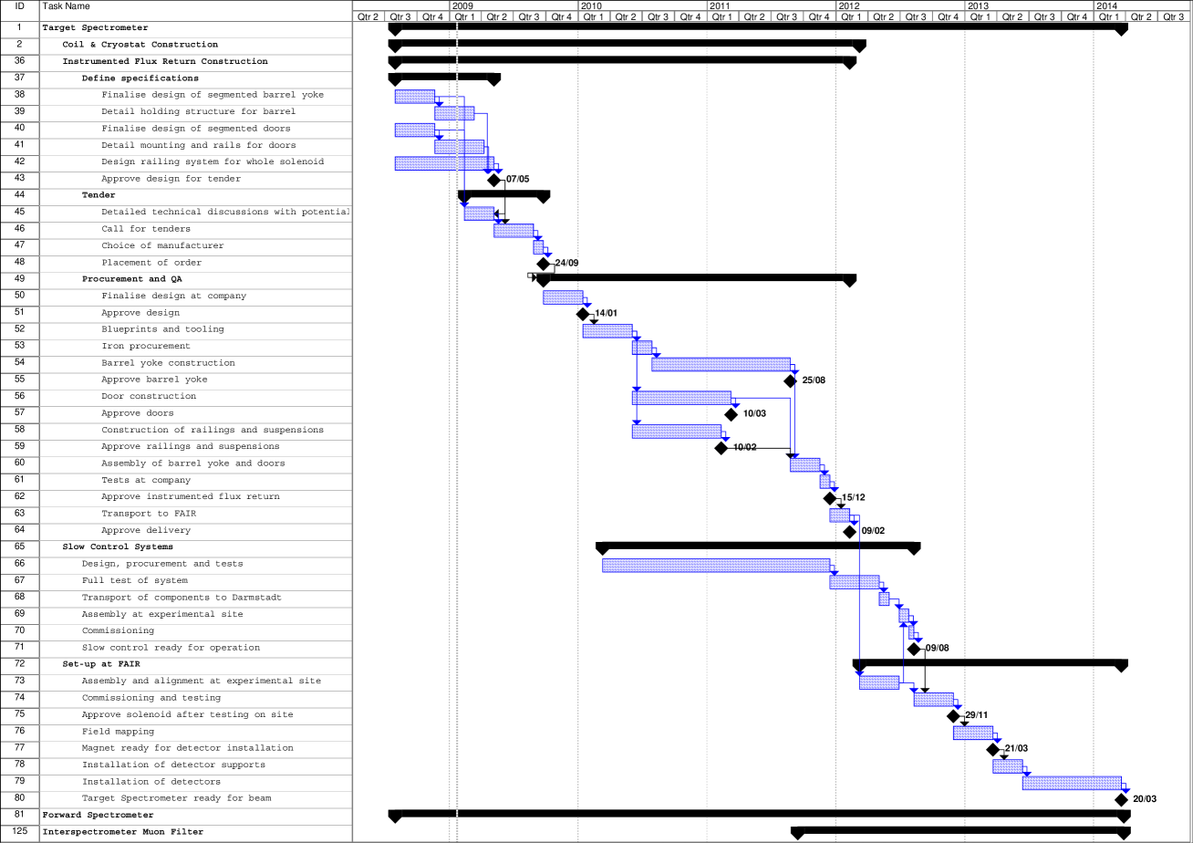
Figure 5.2: Timelines highlighting the instrumented flux return and the slow control systems of the Target Spectrometer.

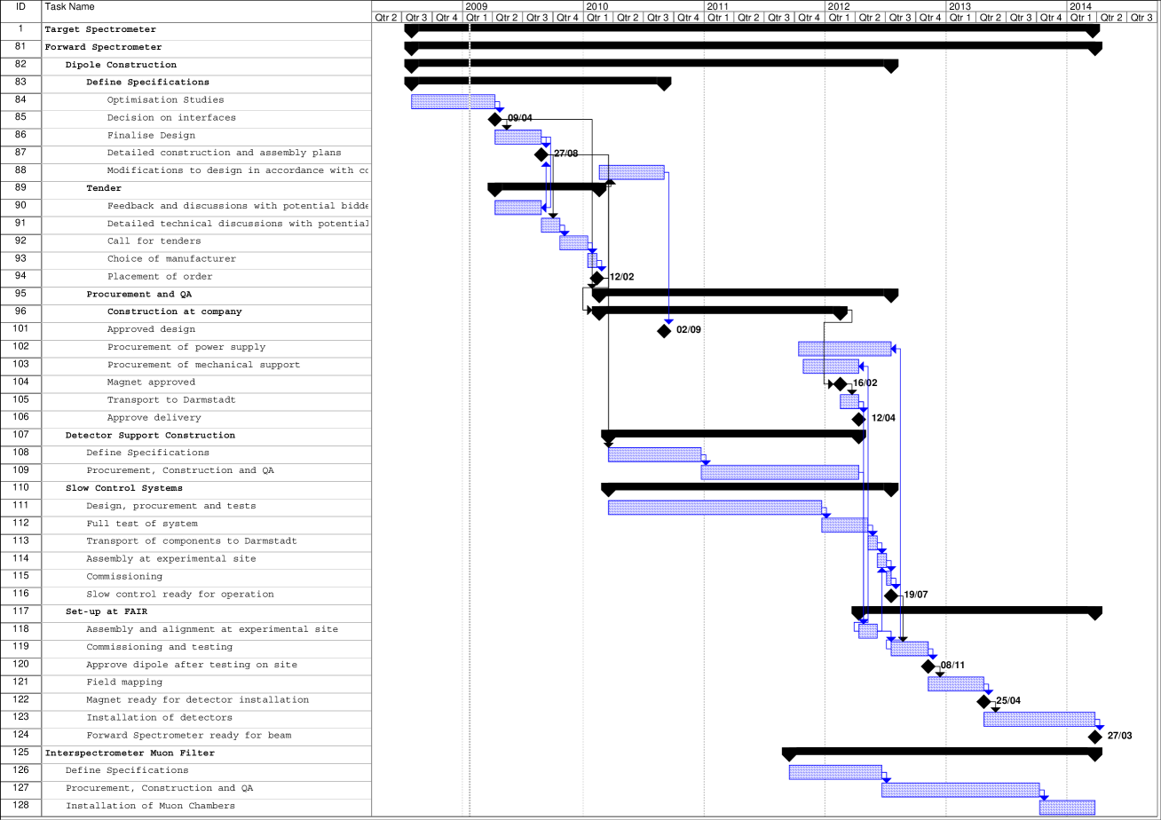
Figure 5.3: Timelines highlighting the Forward Spectrometer and intermediate muon filter.

Acknowledgments
We acknowledge financial support from: the Bundesministerium für Bildung und Forschung (bmbf), the Deutsche Forschungsgemeinschaft (DFG), the University of Groningen, Netherlands, the GSI Helmholtzzentrum für Schwerionenforschung GmbH, Darmstadt, the Helmholtz-Gemeinschaft Deutscher Forschungszentren (HGF), the Schweizerischer Nationalfonds zur Förderung der wissenschaftlichen Forschung (SNF), the Russian funding agency “State Corporation for Atomic Energy Rosatom”, the CNRS/IN2P3 and the Université Paris-sud, the British funding agency “Science and Technology Facilities Council” (STFC), the Instituto Nazionale di Fisica Nucleare (INFN), the Swedish Research Council, the Polish Ministry of Science and Higher Education, the European Community FP6 FAIR Design Study: DIRACsecondary-Beams, contract number 515873, the European Community FP6 Integrated Infrastructure Initiative: HadronPhysics, contract number RII3-CT-2004-506078, the INTAS, and the Deutscher Akademischer Austauschdienst (DAAD).

List of Acronyms

References

- [1] S. Eidelman et al., Phys. Lett. B592, 1 (2004).
- [2] D. E. Acosta et al., Phys. Rev. Lett. 93, 072001 (2004).
- [3] S. K. Choi et al., Phys. Rev. Lett. 91, 262001 (2003).
- [4] PANDA Collaboration, Technical Progress Report, Technical report, FAIR-ESAC, 2005, http://www-panda.gsi.de.
- [5] K. T. Brinkmann, P. Gianotti, and I. Lehmann, Nucl. Phys. News 16, 15 (2006), arXiv:physics/0701090.
- [6] FAIR Project, Baseline Technical Report, Technical report, GSI, Darmstadt, 2006, ISBN: 3-9811298-0-6, EAN: 978-3-9811298-0-9, http://www.gsi.de/fair/reports/btr.html.
- [7] PANDA Collaboration, Physics Performance Report for PANDA, 2009, http://www-panda.gsi.de/archive/public/panda_pb.pdf.
- [8] J. Bai et al., Phys. Rev. Lett. 84, 594200 (2000).
- [9] J. Bai et al., Phys. Rev. Lett. 88, 101802 (2002).
- [10] S. Uehara et al., Phys. Rev. Lett. 96, 082003 (2006).
- [11] K. Abe et al., Phys. Rev. Lett. 94, 182002 (2005).
- [12] G. E. Brown and M. Rho, Phys. Lett. B338, 301 (1994).
- [13] FAIR Project, FAIR Brochure, 2008, http://www.gsi.de/documents/DOC-2008-May-86-1.pdf.
- [14] FAIR Baseline Technical Report, subproject HESR, Technical report, Gesellschaft für Schwerionenforschung (GSI), Darmstadt, 2006, ISBN 3-9811298-0-6.
- [15] FAIR Technical Design Report, HESR, Technical report, Gesellschaft für Schwerionenforschung (GSI), Darmstadt, 2008, http://www-win.gsi.de/FAIR-EOI/PDF/TDR_PDF/TDR_HESR-TRV3.1.2.pdf.
- [16] A. Lehrach et al., Beam dynamics of the High-Energy Storage Ring (HESR) for FAIR, in Conference Proceedings, STORI08, Journal of Modern Physics E.
- [17] V. Parkhomchuk, Nucl. Instrum. Meth. A441, 9 (2000).
- [18] A. Sørensen, in CERN 87-10, 135, 1987.
- [19] F. Hinterberger, T. Mayer-Kuckuk, and D. Prasuhn, Nucl. Instrum. Meth. A275, 239 (1989).
- [20] F. Hinterberger and D. Prasuhn, Nucl. Instrum. Meth. A279, 413 (1989).
- [21] O. Boine-Frankenheim, R. Hasse, F. Hinterberger, A. Lehrach, and P. Zenkevich, Nucl. Instrum. Meth. A560, 245 (2006).
- [22] A. Lehrach, O. Boine-Frankenheim, F. Hinterberger, R. Maier, and D. Prasuhn, Nucl. Instrum. Meth. A561, 289 (2006).
- [23] F. Hinterberger, in Beam-Target Interaction and Intra-beam Scattering in the HESR Ring, Report of the Forschungszentrum Jülich, 2006, Jül-4206, ISSN 0944-2952.
- [24] H. Staengle et al., Nucl. Instrum. Meth. A397, 261 (1997).
- [25] A. Adametz, ”Preshower Measurement with the Cherenkov Detector of the BABAR Experiment Aleksandra Adametz”, Diploma thesis, Master’s thesis, University Heidelberg, 2005.
- [26] K. Mengel et al., IEEE Trans. Nucl. Sci. 45, 681 (1998).
- [27] R. Novotny et al., IEEE Trans. Nucl. Sci. 47, 1499 (2000).
- [28] M. Hoek et al., Nucl. Instrum. Meth. A486, 136 (2002).
- [29] PANDA Collaboration, Technical Design Report, PANDA Electromagnetic Calorimeter (EMC), Technical report, FAIR–GSI, 2008, arXiv:0810.1216 [physics.ins-det].
- [30] N. Akopov et al., Nucl. Instrum. Meth. A479, 511 (2002).
- [31] G. S. Atoyan et al., Nucl. Instrum. Meth. A320, 144 (1992).
- [32] I.-H. Chiang et al., (1999), KOPIO Proposal.
- [33] A. Yamamoto et al., KEK-PREPRINT-85-83.
- [34] H. Minemura et al., Nucl. Instrum. Meth. A238, 18 (1985).
- [35] J. M. Baze et al., In *Boston 1987, Proceedings, Magnet technology* 1260-1263.
- [36] E. Acerbi, F. Alessandria, G. Baccaglioni, and L. Rossi, IN *ZUERICH 1985, PROCEEDINGS, MAGNET TECHNOLOGY*, 163-166.
- [37] H1-PROPOSAL.
- [38] CERN Geneva - CERN-LEPC-83-03 (83,REC.OCT.) 237p.
- [39] A. Yamamoto et al., Nucl. Instrum. Meth. A584, 53 (2008).
- [40] H. Desportes et al., Ad. Cryogenics Eng. 25, 175 (1980).
- [41] Ansoft GmbH, Ansoft GmbH Maxwell Electromagnetic FEM, 12.0 edition, 2008.
- [42] ANSYS INC, General Finite Element Code, 10.0 edition, 2005.
- [43] Vector Fields Ltd., Oxford, UK, OPERA 3D - Software for Electromagnetic Design. TOSCA 9.0 Reference Manual., 2003.
- [44] M. S. Lubell, IEEE Trans on Mag MAG 19, 720 (1983).
- [45] Unfired pressue vessels, 2006, BS EN 13445.
- [46] Design of steel structures, 1993, EuroCode3, EN-1993.
- [47] A. Efremov et al., Nuclear Instruments and Methods in Physics Research A 585, 182 (2008).
- [48] A. Bersani et al., Nuclear Instruments and Methods in Physics Research A 586, 392 (2008).
- [49] E. Koshurnikov et al., IEEE Transactions on Applied Superconductivity 16, 469 (2006).
- [50] M. N. Wilson, Superconducting Magnets, New. York: Clarendon Press, Oxford, 1983.
- [51] LHCb magnet: Technical design report, Technical report, CERN, 2000, CERN-LHCC-2000-007.
- [52] Dassault Systemes, 75008 Paris, CATIA - Computer Aided Three Dimensional Interactive Application. CATIA V5, Reference Manual., r17 edition, 2008.
- [53] Vector Fields Ltd., Oxford, UK, OPERA 3D - Software for Electromagnetic Design. TOSCA 12.0 Reference Manual., x64 edition, 2008.

References

- [1] S. Eidelman et al., Phys. Lett. B592, 1 (2004).
- [2] D. E. Acosta et al., Phys. Rev. Lett. 93, 072001 (2004).
- [3] S. K. Choi et al., Phys. Rev. Lett. 91, 262001 (2003).
- [4] PANDA Collaboration, Technical Progress Report, Technical report, FAIR-ESAC, 2005, http://www-panda.gsi.de.
- [5] K. T. Brinkmann, P. Gianotti, and I. Lehmann, Nucl. Phys. News 16, 15 (2006), arXiv:physics/0701090.
- [6] FAIR Project, Baseline Technical Report, Technical report, GSI, Darmstadt, 2006, ISBN: 3-9811298-0-6, EAN: 978-3-9811298-0-9, http://www.gsi.de/fair/reports/btr.html.
- [7] PANDA Collaboration, Physics Performance Report for PANDA, 2009, http://www-panda.gsi.de/archive/public/panda_pb.pdf.
- [8] J. Bai et al., Phys. Rev. Lett. 84, 594200 (2000).
- [9] J. Bai et al., Phys. Rev. Lett. 88, 101802 (2002).
- [10] S. Uehara et al., Phys. Rev. Lett. 96, 082003 (2006).
- [11] K. Abe et al., Phys. Rev. Lett. 94, 182002 (2005).
- [12] G. E. Brown and M. Rho, Phys. Lett. B338, 301 (1994).
- [13] FAIR Project, FAIR Brochure, 2008, http://www.gsi.de/documents/DOC-2008-May-86-1.pdf.
- [14] FAIR Baseline Technical Report, subproject HESR, Technical report, Gesellschaft für Schwerionenforschung (GSI), Darmstadt, 2006, ISBN 3-9811298-0-6.
- [15] FAIR Technical Design Report, HESR, Technical report, Gesellschaft für Schwerionenforschung (GSI), Darmstadt, 2008, http://www-win.gsi.de/FAIR-EOI/PDF/TDR_PDF/TDR_HESR-TRV3.1.2.pdf.
- [16] A. Lehrach et al., Beam dynamics of the High-Energy Storage Ring (HESR) for FAIR, in Conference Proceedings, STORI08, Journal of Modern Physics E.
- [17] V. Parkhomchuk, Nucl. Instrum. Meth. A441, 9 (2000).
- [18] A. Sørensen, in CERN 87-10, 135, 1987.
- [19] F. Hinterberger, T. Mayer-Kuckuk, and D. Prasuhn, Nucl. Instrum. Meth. A275, 239 (1989).
- [20] F. Hinterberger and D. Prasuhn, Nucl. Instrum. Meth. A279, 413 (1989).
- [21] O. Boine-Frankenheim, R. Hasse, F. Hinterberger, A. Lehrach, and P. Zenkevich, Nucl. Instrum. Meth. A560, 245 (2006).
- [22] A. Lehrach, O. Boine-Frankenheim, F. Hinterberger, R. Maier, and D. Prasuhn, Nucl. Instrum. Meth. A561, 289 (2006).
- [23] F. Hinterberger, in Beam-Target Interaction and Intra-beam Scattering in the HESR Ring, Report of the Forschungszentrum Jülich, 2006, Jül-4206, ISSN 0944-2952.
- [24] H. Staengle et al., Nucl. Instrum. Meth. A397, 261 (1997).
- [25] A. Adametz, ”Preshower Measurement with the Cherenkov Detector of the BABAR Experiment Aleksandra Adametz”, Diploma thesis, Master’s thesis, University Heidelberg, 2005.
- [26] K. Mengel et al., IEEE Trans. Nucl. Sci. 45, 681 (1998).
- [27] R. Novotny et al., IEEE Trans. Nucl. Sci. 47, 1499 (2000).
- [28] M. Hoek et al., Nucl. Instrum. Meth. A486, 136 (2002).
- [29] PANDA Collaboration, Technical Design Report, PANDA Electromagnetic Calorimeter (EMC), Technical report, FAIR–GSI, 2008, arXiv:0810.1216 [physics.ins-det].
- [30] N. Akopov et al., Nucl. Instrum. Meth. A479, 511 (2002).
- [31] G. S. Atoyan et al., Nucl. Instrum. Meth. A320, 144 (1992).
- [32] I.-H. Chiang et al., (1999), KOPIO Proposal.
- [33] A. Yamamoto et al., KEK-PREPRINT-85-83.
- [34] H. Minemura et al., Nucl. Instrum. Meth. A238, 18 (1985).
- [35] J. M. Baze et al., In *Boston 1987, Proceedings, Magnet technology* 1260-1263.
- [36] E. Acerbi, F. Alessandria, G. Baccaglioni, and L. Rossi, IN *ZUERICH 1985, PROCEEDINGS, MAGNET TECHNOLOGY*, 163-166.
- [37] H1-PROPOSAL.
- [38] CERN Geneva - CERN-LEPC-83-03 (83,REC.OCT.) 237p.
- [39] A. Yamamoto et al., Nucl. Instrum. Meth. A584, 53 (2008).
- [40] H. Desportes et al., Ad. Cryogenics Eng. 25, 175 (1980).
- [41] Ansoft GmbH, Ansoft GmbH Maxwell Electromagnetic FEM, 12.0 edition, 2008.
- [42] ANSYS INC, General Finite Element Code, 10.0 edition, 2005.
- [43] Vector Fields Ltd., Oxford, UK, OPERA 3D - Software for Electromagnetic Design. TOSCA 9.0 Reference Manual., 2003.
- [44] M. S. Lubell, IEEE Trans on Mag MAG 19, 720 (1983).
- [45] Unfired pressue vessels, 2006, BS EN 13445.
- [46] Design of steel structures, 1993, EuroCode3, EN-1993.
- [47] A. Efremov et al., Nuclear Instruments and Methods in Physics Research A 585, 182 (2008).
- [48] A. Bersani et al., Nuclear Instruments and Methods in Physics Research A 586, 392 (2008).
- [49] E. Koshurnikov et al., IEEE Transactions on Applied Superconductivity 16, 469 (2006).
- [50] M. N. Wilson, Superconducting Magnets, New. York: Clarendon Press, Oxford, 1983.
- [51] LHCb magnet: Technical design report, Technical report, CERN, 2000, CERN-LHCC-2000-007.
- [52] Dassault Systemes, 75008 Paris, CATIA - Computer Aided Three Dimensional Interactive Application. CATIA V5, Reference Manual., r17 edition, 2008.
- [53] Vector Fields Ltd., Oxford, UK, OPERA 3D - Software for Electromagnetic Design. TOSCA 12.0 Reference Manual., x64 edition, 2008.

References

- [1] S. Eidelman et al., Phys. Lett. B592, 1 (2004).
- [2] D. E. Acosta et al., Phys. Rev. Lett. 93, 072001 (2004).
- [3] S. K. Choi et al., Phys. Rev. Lett. 91, 262001 (2003).
- [4] PANDA Collaboration, Technical Progress Report, Technical report, FAIR-ESAC, 2005, http://www-panda.gsi.de.
- [5] K. T. Brinkmann, P. Gianotti, and I. Lehmann, Nucl. Phys. News 16, 15 (2006), arXiv:physics/0701090.
- [6] FAIR Project, Baseline Technical Report, Technical report, GSI, Darmstadt, 2006, ISBN: 3-9811298-0-6, EAN: 978-3-9811298-0-9, http://www.gsi.de/fair/reports/btr.html.
- [7] PANDA Collaboration, Physics Performance Report for PANDA, 2009, http://www-panda.gsi.de/archive/public/panda_pb.pdf.
- [8] J. Bai et al., Phys. Rev. Lett. 84, 594200 (2000).
- [9] J. Bai et al., Phys. Rev. Lett. 88, 101802 (2002).
- [10] S. Uehara et al., Phys. Rev. Lett. 96, 082003 (2006).
- [11] K. Abe et al., Phys. Rev. Lett. 94, 182002 (2005).
- [12] G. E. Brown and M. Rho, Phys. Lett. B338, 301 (1994).
- [13] FAIR Project, FAIR Brochure, 2008, http://www.gsi.de/documents/DOC-2008-May-86-1.pdf.
- [14] FAIR Baseline Technical Report, subproject HESR, Technical report, Gesellschaft für Schwerionenforschung (GSI), Darmstadt, 2006, ISBN 3-9811298-0-6.
- [15] FAIR Technical Design Report, HESR, Technical report, Gesellschaft für Schwerionenforschung (GSI), Darmstadt, 2008, http://www-win.gsi.de/FAIR-EOI/PDF/TDR_PDF/TDR_HESR-TRV3.1.2.pdf.
- [16] A. Lehrach et al., Beam dynamics of the High-Energy Storage Ring (HESR) for FAIR, in Conference Proceedings, STORI08, Journal of Modern Physics E.
- [17] V. Parkhomchuk, Nucl. Instrum. Meth. A441, 9 (2000).
- [18] A. Sørensen, in CERN 87-10, 135, 1987.
- [19] F. Hinterberger, T. Mayer-Kuckuk, and D. Prasuhn, Nucl. Instrum. Meth. A275, 239 (1989).
- [20] F. Hinterberger and D. Prasuhn, Nucl. Instrum. Meth. A279, 413 (1989).
- [21] O. Boine-Frankenheim, R. Hasse, F. Hinterberger, A. Lehrach, and P. Zenkevich, Nucl. Instrum. Meth. A560, 245 (2006).
- [22] A. Lehrach, O. Boine-Frankenheim, F. Hinterberger, R. Maier, and D. Prasuhn, Nucl. Instrum. Meth. A561, 289 (2006).
- [23] F. Hinterberger, in Beam-Target Interaction and Intra-beam Scattering in the HESR Ring, Report of the Forschungszentrum Jülich, 2006, Jül-4206, ISSN 0944-2952.
- [24] H. Staengle et al., Nucl. Instrum. Meth. A397, 261 (1997).
- [25] A. Adametz, ”Preshower Measurement with the Cherenkov Detector of the BABAR Experiment Aleksandra Adametz”, Diploma thesis, Master’s thesis, University Heidelberg, 2005.
- [26] K. Mengel et al., IEEE Trans. Nucl. Sci. 45, 681 (1998).
- [27] R. Novotny et al., IEEE Trans. Nucl. Sci. 47, 1499 (2000).
- [28] M. Hoek et al., Nucl. Instrum. Meth. A486, 136 (2002).
- [29] PANDA Collaboration, Technical Design Report, PANDA Electromagnetic Calorimeter (EMC), Technical report, FAIR–GSI, 2008, arXiv:0810.1216 [physics.ins-det].
- [30] N. Akopov et al., Nucl. Instrum. Meth. A479, 511 (2002).
- [31] G. S. Atoyan et al., Nucl. Instrum. Meth. A320, 144 (1992).
- [32] I.-H. Chiang et al., (1999), KOPIO Proposal.
- [33] A. Yamamoto et al., KEK-PREPRINT-85-83.
- [34] H. Minemura et al., Nucl. Instrum. Meth. A238, 18 (1985).
- [35] J. M. Baze et al., In *Boston 1987, Proceedings, Magnet technology* 1260-1263.
- [36] E. Acerbi, F. Alessandria, G. Baccaglioni, and L. Rossi, IN *ZUERICH 1985, PROCEEDINGS, MAGNET TECHNOLOGY*, 163-166.
- [37] H1-PROPOSAL.
- [38] CERN Geneva - CERN-LEPC-83-03 (83,REC.OCT.) 237p.
- [39] A. Yamamoto et al., Nucl. Instrum. Meth. A584, 53 (2008).
- [40] H. Desportes et al., Ad. Cryogenics Eng. 25, 175 (1980).
- [41] Ansoft GmbH, Ansoft GmbH Maxwell Electromagnetic FEM, 12.0 edition, 2008.
- [42] ANSYS INC, General Finite Element Code, 10.0 edition, 2005.
- [43] Vector Fields Ltd., Oxford, UK, OPERA 3D - Software for Electromagnetic Design. TOSCA 9.0 Reference Manual., 2003.
- [44] M. S. Lubell, IEEE Trans on Mag MAG 19, 720 (1983).
- [45] Unfired pressue vessels, 2006, BS EN 13445.
- [46] Design of steel structures, 1993, EuroCode3, EN-1993.
- [47] A. Efremov et al., Nuclear Instruments and Methods in Physics Research A 585, 182 (2008).
- [48] A. Bersani et al., Nuclear Instruments and Methods in Physics Research A 586, 392 (2008).
- [49] E. Koshurnikov et al., IEEE Transactions on Applied Superconductivity 16, 469 (2006).
- [50] M. N. Wilson, Superconducting Magnets, New. York: Clarendon Press, Oxford, 1983.
- [51] LHCb magnet: Technical design report, Technical report, CERN, 2000, CERN-LHCC-2000-007.
- [52] Dassault Systemes, 75008 Paris, CATIA - Computer Aided Three Dimensional Interactive Application. CATIA V5, Reference Manual., r17 edition, 2008.
- [53] Vector Fields Ltd., Oxford, UK, OPERA 3D - Software for Electromagnetic Design. TOSCA 12.0 Reference Manual., x64 edition, 2008.

References

- [1] S. Eidelman et al., Phys. Lett. B592, 1 (2004).
- [2] D. E. Acosta et al., Phys. Rev. Lett. 93, 072001 (2004).
- [3] S. K. Choi et al., Phys. Rev. Lett. 91, 262001 (2003).
- [4] PANDA Collaboration, Technical Progress Report, Technical report, FAIR-ESAC, 2005, http://www-panda.gsi.de.
- [5] K. T. Brinkmann, P. Gianotti, and I. Lehmann, Nucl. Phys. News 16, 15 (2006), arXiv:physics/0701090.
- [6] FAIR Project, Baseline Technical Report, Technical report, GSI, Darmstadt, 2006, ISBN: 3-9811298-0-6, EAN: 978-3-9811298-0-9, http://www.gsi.de/fair/reports/btr.html.
- [7] PANDA Collaboration, Physics Performance Report for PANDA, 2009, http://www-panda.gsi.de/archive/public/panda_pb.pdf.
- [8] J. Bai et al., Phys. Rev. Lett. 84, 594200 (2000).
- [9] J. Bai et al., Phys. Rev. Lett. 88, 101802 (2002).
- [10] S. Uehara et al., Phys. Rev. Lett. 96, 082003 (2006).
- [11] K. Abe et al., Phys. Rev. Lett. 94, 182002 (2005).
- [12] G. E. Brown and M. Rho, Phys. Lett. B338, 301 (1994).
- [13] FAIR Project, FAIR Brochure, 2008, http://www.gsi.de/documents/DOC-2008-May-86-1.pdf.
- [14] FAIR Baseline Technical Report, subproject HESR, Technical report, Gesellschaft für Schwerionenforschung (GSI), Darmstadt, 2006, ISBN 3-9811298-0-6.
- [15] FAIR Technical Design Report, HESR, Technical report, Gesellschaft für Schwerionenforschung (GSI), Darmstadt, 2008, http://www-win.gsi.de/FAIR-EOI/PDF/TDR_PDF/TDR_HESR-TRV3.1.2.pdf.
- [16] A. Lehrach et al., Beam dynamics of the High-Energy Storage Ring (HESR) for FAIR, in Conference Proceedings, STORI08, Journal of Modern Physics E.
- [17] V. Parkhomchuk, Nucl. Instrum. Meth. A441, 9 (2000).
- [18] A. Sørensen, in CERN 87-10, 135, 1987.
- [19] F. Hinterberger, T. Mayer-Kuckuk, and D. Prasuhn, Nucl. Instrum. Meth. A275, 239 (1989).
- [20] F. Hinterberger and D. Prasuhn, Nucl. Instrum. Meth. A279, 413 (1989).
- [21] O. Boine-Frankenheim, R. Hasse, F. Hinterberger, A. Lehrach, and P. Zenkevich, Nucl. Instrum. Meth. A560, 245 (2006).
- [22] A. Lehrach, O. Boine-Frankenheim, F. Hinterberger, R. Maier, and D. Prasuhn, Nucl. Instrum. Meth. A561, 289 (2006).
- [23] F. Hinterberger, in Beam-Target Interaction and Intra-beam Scattering in the HESR Ring, Report of the Forschungszentrum Jülich, 2006, Jül-4206, ISSN 0944-2952.
- [24] H. Staengle et al., Nucl. Instrum. Meth. A397, 261 (1997).
- [25] A. Adametz, ”Preshower Measurement with the Cherenkov Detector of the BABAR Experiment Aleksandra Adametz”, Diploma thesis, Master’s thesis, University Heidelberg, 2005.
- [26] K. Mengel et al., IEEE Trans. Nucl. Sci. 45, 681 (1998).
- [27] R. Novotny et al., IEEE Trans. Nucl. Sci. 47, 1499 (2000).
- [28] M. Hoek et al., Nucl. Instrum. Meth. A486, 136 (2002).
- [29] PANDA Collaboration, Technical Design Report, PANDA Electromagnetic Calorimeter (EMC), Technical report, FAIR–GSI, 2008, arXiv:0810.1216 [physics.ins-det].
- [30] N. Akopov et al., Nucl. Instrum. Meth. A479, 511 (2002).
- [31] G. S. Atoyan et al., Nucl. Instrum. Meth. A320, 144 (1992).
- [32] I.-H. Chiang et al., (1999), KOPIO Proposal.
- [33] A. Yamamoto et al., KEK-PREPRINT-85-83.
- [34] H. Minemura et al., Nucl. Instrum. Meth. A238, 18 (1985).
- [35] J. M. Baze et al., In *Boston 1987, Proceedings, Magnet technology* 1260-1263.
- [36] E. Acerbi, F. Alessandria, G. Baccaglioni, and L. Rossi, IN *ZUERICH 1985, PROCEEDINGS, MAGNET TECHNOLOGY*, 163-166.
- [37] H1-PROPOSAL.
- [38] CERN Geneva - CERN-LEPC-83-03 (83,REC.OCT.) 237p.
- [39] A. Yamamoto et al., Nucl. Instrum. Meth. A584, 53 (2008).
- [40] H. Desportes et al., Ad. Cryogenics Eng. 25, 175 (1980).
- [41] Ansoft GmbH, Ansoft GmbH Maxwell Electromagnetic FEM, 12.0 edition, 2008.
- [42] ANSYS INC, General Finite Element Code, 10.0 edition, 2005.
- [43] Vector Fields Ltd., Oxford, UK, OPERA 3D - Software for Electromagnetic Design. TOSCA 9.0 Reference Manual., 2003.
- [44] M. S. Lubell, IEEE Trans on Mag MAG 19, 720 (1983).
- [45] Unfired pressue vessels, 2006, BS EN 13445.
- [46] Design of steel structures, 1993, EuroCode3, EN-1993.
- [47] A. Efremov et al., Nuclear Instruments and Methods in Physics Research A 585, 182 (2008).
- [48] A. Bersani et al., Nuclear Instruments and Methods in Physics Research A 586, 392 (2008).
- [49] E. Koshurnikov et al., IEEE Transactions on Applied Superconductivity 16, 469 (2006).
- [50] M. N. Wilson, Superconducting Magnets, New. York: Clarendon Press, Oxford, 1983.
- [51] LHCb magnet: Technical design report, Technical report, CERN, 2000, CERN-LHCC-2000-007.
- [52] Dassault Systemes, 75008 Paris, CATIA - Computer Aided Three Dimensional Interactive Application. CATIA V5, Reference Manual., r17 edition, 2008.
- [53] Vector Fields Ltd., Oxford, UK, OPERA 3D - Software for Electromagnetic Design. TOSCA 12.0 Reference Manual., x64 edition, 2008.