Detecting Entanglement with Jarzynski’s Equality

Abstract

We present a method for detecting the entanglement of a state using non-equilibrium processes. A comparison of relative entropies allows us to construct an entanglement witness. The relative entropy can further be related to the quantum Jarzynski equality, allowing non-equilibrium work to be used in entanglement detection. To exemplify our results, we consider two different spin chains.

In quantum information theory, entanglement is considered not only an interesting phenomenon, but also a resource which can be used in quantum computation. Entanglement has therefore been the topic of much research. A separable state can be written as a convex sum of pure product states, $\sigma=\sum_{i}p_{i}\sigma_{i}^{1}\otimes\sigma_{i}^{2}\otimes\cdots\otimes\sigma_{i}^{n}$ where the $p_{i}$s are the weights of the product states, $\sigma_{i}^{j}$, with $\sum_{i}p_{i}=1$, while an entangled state cannot. Many methods have been devised to measure and detect entanglement, even for thermal and for many-body systems manybody . The entanglement witness ent_wit is an expectation value of an operator which is bounded for any separable state, whereas entangled states can exceed this bound. A thermodynamic witness allows us to use thermodynamic quantities such as the magnetic susceptibility mag_susc to detect entanglement. The major advantage of using a such a witness is that we can detect thermal many-body entanglement using experimentally measurable quantities.

Thus far, these thermodynamic witnesses have only been used for detecting entanglement in equilibrium systems. However, a result from condensed matter theory, Jarzynski’s equality Jarzynski , allows the change in free energy between two equilibrium states to be related to the non-equilibrium work done needed to drive the system from one state to the other. While the work done can be measured or calculated in an experiment, the change in free energy cannot. Thus Jarzynski’s equality can be used to experimentally estimate the change in free energy during a non-equilibrium process ExpJar . It is the aim of this letter to use Jarzynski’s equality to witness equilibrium entanglement using non-equilibrium processes. Our work also raises the exciting possibility of using this witness to detect entanglement in biological systems.

In our construction of an entanglement witness, we use the relative entropy, a directed distance from an initial state $\rho_{i}$ to a final state $\rho_{f}$, given by

$$S(\rho_{f}||\rho_{i})=tr(\rho_{f}\log\rho_{f})-tr(\rho_{f}\log\rho_{i}).$$ (1)

This is a measure of entanglement VrelEnt when $\rho_{i}=\sigma_{css}$ is the closest separable state to $\rho_{f}$. Formally, we have for the relative entropy of entanglement, $E_{RE}(\rho_{f})=\min_{\rho_{i}\in{\mathcal{S}}}S(\rho_{f}||\rho_{i})$, where we take the minimum over the set of separable states ${\mathcal{S}}$, to find $\sigma_{css}$. The relative entropy can measure entanglement for both equilibrium and non-equilibrium, pure and mixed states, and therefore for thermal, open and closed systems.

We can now construct an entanglement witness using the relative entropy by introducing an arbitrary state $\rho^{*}$. Since the set of separable states is convex, and the relative entropy is a directed distance, if the distance from $\sigma_{css}$ to $\rho$ is larger than the distance from $\rho^{*}$ to $\rho$, then $\rho^{*}$ is entangled. Fig. (1) gives a two dimensional representation of this idea. Hence our witness is

$$S(\rho||\sigma_{css})\geq S(\rho||\rho^{*}).$$ (2)

If $\rho^{*}$ satisfies this inequality, we know it must be entangled. The witness is best when $\rho$ is a pure state and hence is located at the edge of the outer ellipse in Fig. (1). We will refer to this inequality as the relative entropy witness. We note that this witness can detect entanglement in both equilibrium and non-equilibrium states.

Although originally a classical result, it has been shown that Jarzynski’s equality,

$$\langle e^{-\beta{\mathcal{W}}}\rangle=e^{-\beta\Delta F},$$ (3)

where $\beta^{-1}$ is the temperature, ${\mathcal{W}}$ is the work done on the system and $\Delta F$ is the change in free energy between the initial and final equilibrium states, is valid for both open openJnew and closed quantum systems Kurchan2 ; Tasaki ; Mukamel . The brackets $\langle\cdots\rangle$ denote an average over all possible realisations of the work, or trajectories in phase space. Both the path and the rate at which the system is driven are fixed for the equality, though each are arbitrary.

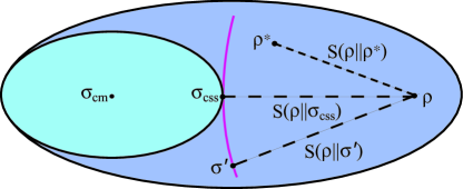
Figure 1: This is a $2$d representation of the multidimensional Hilbert space. The small oval represents the set of separable states, and the large oval the set of all states. $\sigma_{cm}$ is a completely mixed state, and $\sigma_{css}$ is the closest separable state to $\rho$. Any state along the pink curve, such as $\sigma^{\prime}$, has the same “distance” in terms of the relative entropy as $\sigma_{css}$ to $\rho$.

There are several different methods (for a review, see reference Kurchan_rev ), in the literature for deriving a quantum version of Jarzynski’s equality, however we discuss the one which has been successfully theoretically verified Engel . In a closed quantum system, instead of classical trajectories in phase space, we define the quantum equivalent of quantum transition probabilities Kurchan2 ; Tasaki ; Mukamel . An initial Hamiltonian $H_{i}$ and a final Hamiltonian $H_{f}$ have eigenvalues $E_{n}^{i}$, $E_{m}^{f}$ and eigenvectors $|\phi_{n}^{i}\rangle$, $|\phi_{m}^{f}\rangle$ respectively. We perform a measurement of the energy at time $t_{i}$ and then again at $t_{f}$ so that the system is in a specific energy eigenstate. The quantum transition probabilities are then defined as $q_{m,n}=|\langle\phi_{m}^{f}|U(t_{f})|\phi_{n}^{i}\rangle|^{2}$ where $U(t_{f})=\hat{T}_{<}e^{-i\int_{0}^{t_{f}}H(s)ds}$ is the time evolution operator, and $\hat{T}_{<}$ is the time ordering operator. $q_{m,n}$ can be interpreted as the probability that the final state of the system is $|\phi_{m}^{f}\rangle$ given that it was initially in the state $|\phi_{n}^{i}\rangle$. The average is then given as $\langle e^{-\beta{\mathcal{W}}}\rangle=\sum_{n}(e^{-\beta E_{n}^{i}}/Z_{i})\sum_{m}q_{m,n}e^{-\beta(E_{m}^{f}-E_{n}^{i})}$ where the work is defined as ${\mathcal{W}}=E_{m}^{f}-E_{n}^{i}$ and $Z_{i}=tr(e^{-\beta H_{i}})$ is the initial partition function.

Consider now an open quantum system (subsystem, $S$) interacting with a bath, $B$, with total Hamiltonian $H(t)=H_{S}(t)+H_{SB}+H_{B}$ and arbitrary coupling, $H_{SB}$ openJnew . As only the subsystem is time dependent, the change in energy of the total system equals the work done on the subsystem. Hence the average in equation (3) is identical to the closed system case. Further, the free energy of the total system is given by $F(t)=F_{S}(t)+F_{B}$. This allows Jarzynski’s equality to be written $\langle e^{-\beta{\mathcal{W}}}\rangle=e^{-\beta\Delta F_{S}}$ openJnew .

Other fluctuation theorems have also been derived. One equality which will be useful Tasaki is $\langle e^{-(\beta_{f}E_{f}-\beta_{i}E_{i})}\rangle=e^{-(\beta_{f}F_{f}-\beta_{i}F_{i})}$. This demonstrates that a change in temperature between the initial and final state can also be taken into account. However, unless $\beta_{i}=\beta_{f}$, the quantity $(\beta_{f}E_{f}-\beta_{i}E_{i})$ no longer relates to work. We refer to this equation as the Jarzynski-Tasaki equality.

Consider again the relative entropy, equation (1). We now restrict each of the states to be in thermal equilibrium. Thus we have initial and final states, $\sigma_{css}=e^{-\beta_{i}H_{i}}/Z_{i}$ and $\rho=e^{-\beta_{f}H_{f}}/Z_{f}$ respectively. Similarly, $\rho^{*}=e^{-\beta^{*}H^{*}}/Z^{*}$. Expanding equation (1), we can write the relative entropy in terms of a change in free energy donald ; vlatko_land , $S(\rho||\sigma_{css})=\Delta(\beta F)-tr(\rho_{f}\Delta(\beta H))$ where $\Delta(\beta F)=\beta_{f}F_{f}-\beta_{i}F_{i}$ and $\Delta(\beta H)=\beta_{f}H_{f}-\beta_{i}H_{i}$. Combining this identity with the Jarzynski-Tasaki equality, we find that

$$S(\rho||\sigma_{css})=-tr(\rho\Delta(\beta H))-\ln\langle e^{-(\beta_{f}E_{f}-\beta_{i}E_{i})}\rangle.$$ (4)

Equation (4) relates the entanglement to the average change in energy at different temperatures (in a possibly driven system). When $\beta_{f}=\beta_{i}$, we can instead relate the entanglement to the average work done in creating the quantum correlations of $\rho$ from the purely classical correlations of $\sigma_{css}$. In addition to this being an interesting result in itself, we can also use this definition of the relative entropy in the entanglement witness, equation (2). We call this the relative Jarzynski witness and discuss this in more detail below.

An open quantum system (or subsystem) can also be considered. As discussed previously, such systems also obey Jarzynski’s equality, $\langle e^{-\beta{\mathcal{W}}}\rangle=e^{-\beta\Delta F_{S}}$ where $F_{S}(t)$ is the free energy of the subsystem. We define $Y(t)=tr(e^{-\beta(H_{S}(t)+H_{SB}+H_{B})})$ as the partition function of the total system and $Z_{B}=tr(e^{-\beta H_{B}})$ as the partition function of the bath. The partition function of the subsystem, $Z_{S}(t)=tr(e^{-\beta F_{S}})=Y(t)/Z_{B}$ can be associated with an effective Hamiltonian openJnew ,

$$H^{eff}(t)=-\frac{1}{\beta}\ln\left[\frac{tr_{B}(e^{-\beta(H_{S}(t)+H_{SB}+H_{B})})}{tr_{B}(e^{-\beta H_{B}})}\right],$$ (5)

so that $Z_{S}(t)=tr_{S}(e^{-\beta H^{eff}(t)})$. Using these equations, and since the initial and final states must be in equilibrium, we have $\rho_{S}=e^{-\beta H^{eff}(t)}/Z_{S}(t)$ for each state. This only represents the state of the system when it is in equilibrium.

The relative entropy can now be defined in terms of the effective Hamiltonian and the work done on the subsystem, $S(\rho_{S}||\sigma_{S,css})=-\beta tr[\rho_{S}(H_{f}^{eff}-H_{i}^{eff})]-\ln\langle e^{-\beta{\mathcal{W}}}\rangle$. Hence we can write the entanglement witness for an open quantum system, $S(\rho_{S}||\sigma_{S,css})\geq S(\rho_{S}||\rho_{S}^{*})$, where $\rho_{S}^{*}=e^{-\beta H^{eff,*}}/Z_{S}^{*}$ as the state is in equilibrium.

We have shown that it is possible to detect entanglement in a state $\rho^{*}$ or $\rho_{S}^{*}$ using a non-equilibrium process. There are three ways we can use the entanglement witness. First, if we have a specific state $\rho^{*}$ in mind but don’t know whether it is entangled, the witness allows us to detect entanglement in this state. Second, if we have the Hamiltonian of a system, we can detect entanglement in that system. We ask for which values of the parameters of the system, such as a magnetic field, is the system entangled? In this case we find out in which $\rho^{*}$s of the system entanglement can be detected. Computationally, linking equation (2) to Jarzynski’s equality simply gives a different way to calculate the relative entropy. It is in the third method, the experimental applications, that are exciting in this respect.

Experimentally, we can relate the relative Jarzynski witness to non-equilibrium processes. For the closed quantum system when $\beta_{f}=\beta_{i}$, and the open quantum system, this corresponds to a series of measurements. We drop the subscript $S$ that denotes the subsystem in the open quantum system here since the work done in the open system is equal to the change in energy of the total, closed, system. Hence the discussion is valid for both open and closed systems.

Since we consider a quantum system, measurements of the energy on many replicas of the same system will give different values. As the quantum Jarzynski equality demonstrates, each time we measure an initial and a final energy of a system to calculate the work, we obtain different results. After many measurements of the initial state ($\sigma_{css}$) and the final state ($\rho$), we can calculate the average $\langle e^{-\beta{\mathcal{W}}}\rangle$. We then repeat this procedure with initial state $\rho^{*}$ and compare the resulting experimental values of the relative entropy. The value of $tr(\rho(H_{f}-H_{i}))$ can also be experimentally measured. For instance, if a magnetic field is driving the process, this corresponds to the change in the field multiplied by the final state magnetisation. We can now detect entanglement in $\rho^{*}$.

When $\beta_{f}\neq\beta_{i}$ we can use the Jarzynski-Tasaki equality and a similar argument holds. However, it is no longer the work done that is measured. Instead we measure the initial and final temperatures of the system in addition to the energy eigenvalues.

A problem with using our Jarzynski witness is the possibility that $\sigma_{css}$ is not an equilibrium state of the system, and therefore we cannot define Jarzynski’s equality. However, we find that we do not require $\sigma_{css}$ to be in equilibrium itself. Instead, we require only that we have an equilibrium state $\sigma^{\prime}$ of the system where $S(\rho||\sigma_{css})=S(\rho||\sigma^{\prime})$. The states satisfying this equality are represented by the pink curve in Fig. (1).

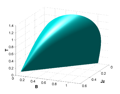
Figure 2: This plots $J_{z}$ versus $B$ and $T$ when $N=3$, and shows the values for which we can detect entanglement in $\rho^{*}$. The state is entangled between the surface of the plot and the axes.

We now illustrate the entanglement witness with two examples. We first consider a three qubit $XXZ$ spin chain as we can define both the initial and final states to be in equilibrium. In the second example, we use a seven qubit chain to demonstrate what happens when the closest separable state is not in equilibrium and we must use a different equilibrium state $\sigma^{\prime}$.

For each example, we have calculated the witness using the relative entropy witness and using the Jarzynski-Tasaki witness, and find both give the correct results. This also allows us to successfully numerically verify the Jarzynski-Taskaki equality. We calculate the time evolution operator exactly in the three qubit case as $[H(t_{1}),H(t_{2})]=0$, and using the method described in Dorosz for seven qubits as $[H(t_{1}),H(t_{2})]\neq 0$. This method allows an approximation of $U(t_{f})$ to be calculated using $U(t_{f})=\prod_{n=0}^{M-1}e^{-iH(t_{n})\Delta t}$. We use $\Delta t=0.001$ to give accurate results. We use these examples rather than that of an open quantum system since the closest separable state to $\rho_{n}$ given below is known. This allows us to do some of the calculation analytically which allows further insight into the problem.

We take our state to be close to the pure symmetric state, $\rho_{n}=(1/n)\hat{S}(|00\cdots 01\rangle)\hat{S}(\langle 00\cdots 01|)$ where $\hat{S}$ is the total symmetrisation operator, whose closest separable state vlatko_css ; wei_css is known to be

$$\sigma_{css,n}=\frac{1}{n^{n}}\sum_{k=0}^{n}(n-1)^{k}\hat{S}(|\underbrace{000}_{k}...\underbrace{111}_{n-k}\rangle)\hat{S}(\langle\underbrace{000}_{k}...\underbrace{111}_{n-k}|).$$ (6)

We will identify the states $\rho_{n}$ and $\sigma_{css,n}$ with thermal equilibrium states, $e^{-\beta H}/Z$, and hence we will not have exactly the states above. However, we find that the relative entropy calculated in each case is identical to many significant figures.

The Hamiltonian of the $XXZ$ spin chain is

$$H=-\sum_{l=1}^{n}\left[\frac{J}{2}\left(\sigma_{l}^{x}\sigma_{l+1}^{x}+\sigma_{l}^{y}\sigma_{l+1}^{y}\right)+J_{z}\sigma_{l}^{z}\sigma_{l+1}^{z}+B\sigma_{l}^{z}\right],$$ (7)

where $J$ and $J_{z}$ are coupling strengths, and $B$ is a magnetic field.

For our first example, the three qubit spin chain, we require $J_{z}$ and $B$ to be time dependent. Both $\rho_{3}$ and $\sigma_{css,3}$ can be written as thermal equilibrium states, $\rho=e^{-\beta H}/Z$, of the Hamiltonian. For the initial state to be $\sigma_{css,3}$, we require that $B_{i}=\beta^{-1}\log(2)/2$ and $J_{z,i}=(2J-\beta^{-1}\log(3))/4$ at a low temperature. For concreteness, we take $\beta^{-1}=0.01$ and $J=1$. For the final state to be $\rho_{3}$, we have $B_{f}=1/2$ and $J_{z,f}=0$.

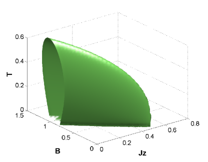
Figure 3: This plots $J_{z}$ versus $B$ and $T$ when $N=7$, and shows the values for which we can detect entanglement in $\rho^{*}$. The state is entangled between the surface of the plot and the axes.

We can now detect entanglement in an arbitrary equilibrium state, $\rho^{*}_{3}$ using the entanglement witness. Fig. (2) shows the values of the magnetic field, $J_{z}$ and the temperature for which we can detect entanglement: we can detect that $\rho^{*}_{3}$ is entangled in the region between the surface and the axes. Hence, experimentally driving a system from the state $\rho^{*}_{3}$ with values of $B$, $J_{z}$ and $T$ that are within the surface to the state $\rho$ will allow entanglement to be detected on comparison with the same process starting at $\sigma_{css,3}$.

Our second example is the $7$ qubit spin chain, with $B$ time dependent and $J_{z}=0$. For any $7$ qubit chain, we cannot identify $\sigma_{css,7}$ with a thermal equilibrium state, and hence we use $\sigma_{7}^{\prime}=[(7^{7}-7\times 6^{6})|0000000\rangle\langle 0000000|+6^{6}\hat{S}(|0000001\rangle)\hat{S}(\langle 0000001|)]/7^{7}$ instead. For the initial state to be $\sigma_{7}^{\prime}$, we require that $B_{i}=\beta^{-1}\log[70993/46656]/2+J$ at a low temperature. For concreteness, we again take $\beta^{-1}=0.01$ and $J=1$, and for the final state to be $\rho_{7}$, we have $B_{f}=0.92$.

We can now detect the entanglement of a state $\rho^{*}_{7}$ as before. Fig. (3) shows the values of $B$, $J_{z}$ and the temperature for which we can detect entanglement. Again, we can detect that $\rho^{*}_{7}$ is entangled in the region between the surface and the axes.

We note that although $J_{z}=0$ for both the initial and final state Hamiltonians, this is not necessarily so for $\rho^{*}$. Indeed, we can detect when $\rho^{*}$ is entangled in many other situations. This is due to the fact that the Hilbert space of the Hamiltonian is spanned by the set of $n$ computational eigenvectors, $\{|00\cdots 0\rangle,|00\cdots 01\rangle\cdots|11\cdots 1\rangle\}$. Hence the entanglement witness applies to any state $\rho^{*}$ that exists within this Hilbert space. For example, we could introduce a Dzyaloshinskii-Moriya interaction to the Hamiltonian of $\rho^{*}$ and still use the witness to detect entanglement in the system.

A possible application of this work is the detection of entanglement in biological systems. The photosynthetic bacteria, Prosthecochloris aestuarii, can be modelled using a seven spin Hamiltonian. Using experimental values adolphs ; plenio and simplifying the model to an isolated system, we can use this Hamiltonian to construct a specific state $\rho^{*}$. The $7$ qubit chain defined above can then be used in the witness. In this simplified model, we do not detect any entanglement. However, we expect that the full model, and a more appropriate Hamiltonian $H_{f}$ which is closer to $H^{*}$ will allow entanglement to be detected.

We have presented a witness which uses the relative entropy to detect entanglement. When the states are in equilibrium, we have shown that Jarzynski’s equality can be used to detect entanglement. Hence this witness enables entanglement to be detected using non-equilibrium processes. Using this witness, we have considered two examples. In one we can define an equilibrium closest separable state to $\rho$, and in the other we instead define an entangled equilibrium state which has the same directed distance to $\rho$ in terms of the relative entropy.

Acknowledgements: V.V. and J.H. acknowledge the EPSRC for financial support. V.V. is grateful for funding from the Wolfson Foundation, the Royal Society and the E.U. His work is also supported by the National Research Foundation and the Ministry of Education (Singapore).

References

- (1) L. Amico, R. Fazio, A. Osterloh and V. Vedral, Rev. Mod. Phys. 80, 517 (2008)
- (2) G. Toth, Phys. Rev. A 71, 010301(R) (2005)
- (3) M. Wiesniak, V. Vedral and C. Brukner, New J. Phys. 7, 258 (2005)
- (4) C. Jarzynski, Phys. Rev. Lett. 78, 2690 (1997)
- (5) J. Liphardt, S. Dumont, S. B. Smith, I. Tinoco, Jr., and C. Bustamante Science 296, 1832 (2002).
- (6) V. Vedral, M. B. Plenio, M. A. Rippin, and P. L. Knight, Phys. Rev. Lett. 78, 2275 (1997)
- (7) M. Campisi, P. Talkner, and P. Hanggi, Phys. Rev. Lett. 102, 210401 (2009)
- (8) J. Kurchan, arXiv: cond-mat/0007360
- (9) H. Tasaki, arXiv: cond-mat/0009244
- (10) S. Mukamel, Phys. Rev. Lett. 90 170604 (2003)
- (11) J. Kurchan, J. Stat. Mech. P07005 (2007)
- (12) A. Engel and R. Nolte, Europhys. Lett. 79, 10003 (2007)
- (13) M. J. Donald, J. Stat. Phys. 49, 81 (1987).
- (14) V. Vedral, Proc. R. Soc. Lond. A 456, 969 (2000)
- (15) S. Dorosz, T. Platini and D. Karevski, Phys. Rev. E, 77, 051120 (2008)
- (16) V. Vedral, New J. Phys. 6, 102 (2004)
- (17) T. C. Wei, M. Ericsson, P. M. Goldbart and W. J. Munro, Quantum Inf. Comput. 4, 252 (2004)
- (18) M. B. Plenio and S. F. Huelga, New J. Phys. 10, 113019 (2008)
- (19) J. Adolphs and T. Renger, Biophys. J. 91, 2778 (2006)