Abstract

It is shown how a recently proposed method of cloaking is effective over a broad range of frequencies. The method is based on three or more active devices. The devices, while not radiating significantly, create a “quiet zone” between the devices where the wave amplitude is small. Objects placed within this region are virtually invisible. The cloaking is demonstrated by simulations with a broadband incident pulse.

OCIS codes: (260.0260) Physical optics; (350.7420) Waves; (160.4760) Optical properties

1 Introduction

A tremendous amount of interest and excitement has been generated by recent strides towards making objects invisible, not by camouflage, but by manipulating the fields in such a way that the cloaking device and the object to be cloaked scatter very little radiation in any direction and do not absorb it. Here using a new method of active exterior cloaking, described in [1] for single frequency waves, we demonstrate how an object can be cloaked against an incoming broadband pulse. To our knowledge this is the first example showing cloaking of an object against an incoming pulse. It uses active cloaking devices to generate anomalous localized waves which cancel the incident waves within the cloaking region to create a “quiet zone”, within which objects can be hidden. Because active devices, rather than materials, are used to generate the anomalous localized waves, one may superimpose the results for different frequencies to obtain broadband cloaking. Our method requires one to know the form of the incoming pulse in advance, since the fields generated by the cloaking devices are tailored to the incoming fields.

Dolin [2], Kerker [3], and Alú and Engheta [4] realized that certain objects could be made invisible by coating them with an appropriate material tailored according to the object to be cloaked. A breakthrough came with the work of Greenleaf et al.[5], for conductivity, Leonhardt [6], for geometric optics, and Pendry et al.[7] for electromagnetism who showed that materials could guide fields around a region, leaving a “quiet” zone in that region within which objects could be placed without disturbing the surrounding field. This idea was extended to acoustics [8, 9, 10, 11], elastodynamics [12], and water waves [13], and has been confirmed experimentally [14, 13, 15, 16, 17].

A completely different type of cloaking, which we call exterior cloaking because the cloaking region is outside the cloaking device, was introduced by Milton, Nicorovici, McPhedran and collaborators [18, 19, 20]. They showed that clusters of polarizable dipoles within a critical distance of a flat or cylindrical superlens [21, 22, 23] are cloaked. Anomalously localized fields generated by the interaction between the induced dipoles and the superlens effectively cancel the fields acting on the polarizable dipoles. While larger objects do not appear to be cloaked [24], Lai et al.[25] show that an object outside a superlens can be cloaked if the appropriate “antiobject” is embedded in the superlens.

Ideally cloaking should be over a broad range of frequencies. Most cloaking methods are narrowband and approaches to obtain broadband cloaking can have drawbacks, such as requiring frequency independent relative dielectric constants or relative refractive indices less than one [26, 27, 15, 16, 17] which necessitate a surrounding medium with dielectric constant sufficiently greater than one: thus such electromagnetic cloaking could work underwater or in glass, but not in air or space. One proposal without this drawback is the broadband interior cloaking scheme of Miller [28] which uses active cloaking controls rather than passive materials. Here we also use active cloaking devices to achieve broadband exterior cloaking. The principle is similar to that of active sound control (see e.g [29, 30]), with the fundamental novelty that we do not need a closed surface to suppress the incident field in a region while not radiating significantly. Another type of broadband exterior cloaking, using waveguides to guide waves around a “quiet zone”, has recently been introduced and confirmed experimentally [31].

2 Cloaking a single frequency

For simplicity we just consider the two dimensional case, corresponding to transverse electric or magnetic waves, so the governing equation is the Helmholtz equation $\Delta u+k^{2}u=0$. Here $u({\bf x},\omega)$ is the wave field, $k=2\pi/\lambda$ is the wavenumber and $\lambda=2\pi c_{0}/\omega$ is the wavelength at frequency $\omega$ and at a constant propagation speed $c_{0}$. We would like to cloak a region in the plane from a known probing (incident) wave $u_{i}({\bf x},\omega)$ supported in the frequency band $\omega_{0}+[-B/2,B/2]$, where the central frequency is $\omega_{0}$ and the bandwidth is $B$.

The key to our cloaking method are devices that (a) cancel the probing wave in the region to be cloaked and (b) radiate very little waves away from the devices. To give a concrete example, let us take for the cloaked region the disk $|{\bf x}|\leq\alpha$ and assume we measure the radiation emitted by the devices on the circle $|{\bf x}|=\gamma>\alpha$. Thus the device’s field $u_{d}({\bf x},\omega)$ must be so that (a’) $u_{d}\approx-u_{i}$ for $|{\bf x}|\leq\alpha$ and (b’) $u_{d}\approx 0$ for $|{\bf x}|=\gamma$.

The devices can be idealized by $D$ points ${\bf x}_{1},\ldots,{\bf x}_{D}$ with $|{\bf x}_{j}|=\delta$ and $\alpha<\delta<\gamma$ so that the devices surround the cloaked region. Because the device’s field must solve Helmholtz equation and become small far away, we take it as a linear combination of outgoing waves emanating from the source points ${\bf x}_{1},\ldots,{\bf x}_{D}$ with the form [1]:

$$u_{d}({\bf x},\omega)=\sum_{m=1}^{D}\sum_{n=-N}^{N}b_{m,n}H^{(1)}_{n}(k|{\bf x}-{\bf x}_{m}|)\exp[in\theta_{m}],$$

where $H^{(1)}_{n}$ is the $n-$th Hankel function of the first kind and $\theta_{m}\equiv\arg({\bf x}-{\bf x}_{m})$ is the angle between ${\bf x}-{\bf x}_{m}$ and $(1,0)$. We seek coefficients $b_{m,n}$ so that (a’) holds on points of the circle $|{\bf x}|=\alpha$ and (b’) holds on points of the circle $|{\bf x}|=\gamma$. The control points are uniformly distributed and at most $\lambda/2$ apart on each circle. The resulting linear equations are solved in the least squares sense with the Truncated Singular Value Decomposition in two steps. First we find coefficients $b_{m,n}$ so that (a’) holds, and second we find a correction to enforce (b’) while still satisfying (a’). (see Appendix A for more details).

3 Simulations

We demonstrate cloaking in a regime that could correspond to Transverse Electric microwaves in air (neglecting dispersion and attenuation), where $u({\bf x},\omega)$ is the transverse component of the electric field. For the numerical experiments we took a central frequency and bandwidth of $2.4$GHz, a propagation speed of $c_{0}=3\times 10^{8}$m/s and a central wavelength of $\lambda_{0}=12.5$cm. Simulations suggest a minimum of three devices are needed to cloak independently of the direction of the incoming waves. In Fig. 1 we show cloaking at the central frequency $\omega_{0}/(2\pi)=2.4$GHz of a region of radius $\alpha=2\lambda_{0}$ (solid white circle). Here the devices are located $\delta=10\lambda_{0}$ from the origin and invisibility is enforced at a distance $\gamma=20\lambda_{0}$ from the origin (dashed white circle). The incident wave is a point source originating at ${\bf x}_{s}=(-20,0)\lambda_{0}$ and modulated in frequency by a Gaussian truncated to the bandwidth $\widehat{g}(\omega)=\sigma\sqrt{2\pi}\exp(-\sigma^{2}(\omega-\omega_{0})^{2}/2)$, for $|\omega-\omega_{0}|\leq B/2,$ and $0$ otherwise. We took $\sigma=4/\omega_{0}$. The scatterer is a perfectly conducting “kite” obstacle [32] with homogeneous Dirichlet boundary conditions, fitting inside the cloaked region. The scattered field is computed using the boundary integral equation method in [32].

With the devices inactive (Fig. 1a), the “kite” scatters the incident field and thus can be easily detected. When the devices are active (Fig. 1b) they create a region with very small fields while being nearly undetectable from far away. Since there are almost no waves in the cloaked region, the scattered waves from the object are greatly reduced, making the object invisible. Quantitatively, the disturbance of the incident wave is $1.1\times 10^{-4}$% of the field scattered without the devices, as measured on the dashed white circle with the $L^{2}$ norm. We carried the same procedure for $N_{freq}=101$ frequencies in the bandwidth with similar results, as can be seen in Fig. 2. Since the bandwidth is $100$% of the central frequency, broadband cloaking is possible with our approach.

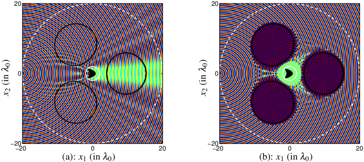
Fig. 1: Wave field at the central frequency $\omega_{0}$ when the cloaking devices are (a) inactive and (b) active. Only the real part of the fields is displayed, with a linear color scale going from $-1$ (dark blue) to $1$ (dark red). All fields have been rescaled by $|u_{i}({\bf x},\omega)|$ to remove the geometric spreading of the point source.

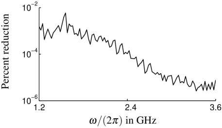
Fig. 2: Reduction of the scattering in percent achieved by the cloaking devices over the bandwidth, measured in the $L^{2}$ norm on $|{\bf x}|=20\lambda_{0}$. The ordinates scale is logarithmic.

Several time snapshots (computed by taking the inverse Fourier transform in time of the total fields) appear in Fig. 3. For full animations see Fig. 3 (Movie 1 and Movie 2), which covers the time interval $[0,T]$, with $T\approx 132$ns or the time it takes for the wave to travel $50.5\lambda_{0}$. The devices make the incoming wave disappear when it reaches the cloaked region, and then rebuild the wave as it exits the cloaked region. This makes the object virtually undetectable.

Here the cloaked region is for visualization purposes deliberately small ($2\lambda_{0}=25$cm radius). However we have successfully cloaked regions up to $10\lambda_{0}=1.25$m in radius as shown in Fig. 4, where we take three devices with $|{\bf x}_{m}|=\delta=5\alpha$ and invisibility is enforced on $|{\bf x}|=\gamma=10\alpha$.

The point-like devices could be problematic in practice because of the ${\cal O}(|{\bf x}-{\bf x}_{m}|^{-N})$ singularities near the devices. Fortunately the point devices can be replaced (with Green’s identities) by curves where the fields have reasonable amplitudes and where we can control a single- and double-layer potential [32]. These curves could be the circles suggested by the contours $\left|{u_{d}}\right|=100\max_{|{\bf x}|=\alpha}|u_{i}({\bf x},\omega)|$ (in black in Fig. 1). The radius of such devices for other cloaked region radii is estimated in Fig. 5. Since the devices do not completely surround the region to be cloaked, exterior cloaking is possible at least for $\alpha\leq 10\lambda_{0}$.

A theoretical study of this cloaking method is ongoing, and we speculate it generalizes to three dimensions and Maxwell equations.

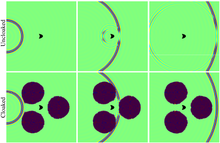
Fig. 3: Cloaking for a circular wave pulse. Top row: devices inactive (Movie 1). Bottom row: devices active (Movie 2). The visualization window in ${\bf x}$ is as in Fig. 1 and the scale is linear and relative to the maximum amplitude on the plane of the incident field at each time.

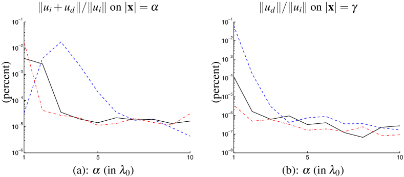
Fig. 4: Cloak performance in terms of the cloaked region radius $\alpha$, as measured by (a) $\|u_{i}+u_{d}\|/\|u_{i}\|$ with the $L^{2}$ norm on $|{\bf x}|=\alpha$ and (b) $\|u_{d}\|/\|u_{i}\|$ with the $L^{2}$ norm on $|{\bf x}|=\gamma$. Dashed, solid and dash-dotted lines correspond to $\omega/(2\pi)=$ $1.2$GHz, $2.4$GHz and $3.6$GHz.

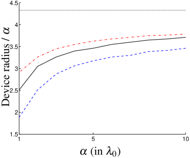
Fig. 5: Estimate of the radius of circular cloaking devices relative to the radius of the cloaked region $\alpha$. Dashed, solid and dash-dotted lines correspond to $\omega/(2\pi)=$ $1.2$GHz, $2.4$GHz and $3.6$GHz, respectively. The device radius is estimated as the largest of the distances from a device point ${\bf x}_{m}$ to the level-set $\left|{u_{d}}\right|=100\max_{|{\bf x}|=\alpha}|u_{i}({\bf x},\omega)|$. If the devices were perfect circles, any device radius below the dotted line (at $\cos(\pi/6)\delta/\alpha=5\sqrt{3}/2$) would indicate that the devices do not touch, i.e. they are three disjoint devices.

Appendix A Finding the driving coefficients for the devices

Let ${\bf b}$ be a vector with the $(2N+1)D$ possibly complex coefficients $b_{m,n}$. Denote by ${\bf p}_{j}^{\alpha}$ (resp. ${\bf p}_{j}^{\gamma}$) the $N^{\alpha}$ (resp. $N^{\gamma}$) control points on the circle $|{\bf x}|=\alpha$ (resp. $|{\bf x}|=\gamma)$. The coefficients ${\bf b}$, the number $N$ of terms in the expression for $u_{d}$ and the control points all depend on the frequency $\omega$. Using the form for $u_{d}$ in the text, construct a matrix ${\bf A}$ of size $N^{\alpha}\times(2N+1)D$ and a matrix ${\bf B}$ of size $N^{\gamma}\times(2N+1)D$ such that $u_{d}({\bf p}_{j}^{\alpha},\omega)=({\bf A}{\bf b})_{j}$ and $u_{d}({\bf p}_{j}^{\gamma},\omega)=({\bf B}{\bf b})_{j}$. We estimate the driving coefficients as follows. Enforce (a’): Use the Truncated Singular Value Decomposition (TSVD) to find coefficients ${\bf b}_{0}$ such that ${\bf A}{\bf b}_{0}\approx-[u_{i}({\bf p}_{j}^{\alpha},\omega)]$, in the least squares sense. Enforce (b’) while still satisfying (a’): Find ${\bf z}$ as the solution to the least squares problem ${\bf B}({\bf b}_{0}+{\bf Z}{\bf z})\approx\mathbf{0}$. Again the TSVD can be used for this step. Here ${\bf Z}$ is a matrix with columns spanning the nullspace of ${\bf A}$ (a byproduct of the SVD in the previous step).

The coefficients are then ${\bf b}={\bf b}_{0}+{\bf Z}{\bf z}$. The heuristic for $N$ in the numerical experiments is $N=\lceil{k(\delta-\alpha/2)}\rceil$, where $\lceil{x}\rceil$ is the smallest integer larger than $x$. The choice of cut-off singular values can be used to control how well one wants to satisfy (a’) and (b’). We used a fixed $10^{-5}$ tolerance relative to the maximum amplitude of $u_{i}$ on the control points.