Reexamination of Astrophysical Resonance-Reaction-Rate Equations for An Isolated, Narrow Resonance

Abstract

The well-known astrophysical resonant-reaction-rate (RRR) equations for an isolated narrow resonance induced by the charged particles have been reexamined. The validity of those ‘look reliable’ assumptions used in deriving the classical analytic equations has been checked, and found that these analytic equations only hold for certain circumstances. It shows the customary definition of ‘narrow’ is inappropriate or ambiguous in some sense, and it awakes us not to use those analytic equations without caution. As a suggestion, it’s better to use the broad-resonance equation to calculate the RRR numerically even for a narrow resonance. The present conclusion may influence some work in which the classical narrow-resonant equations were used for calculating the RRRs, especially at low stellar temperatures for those previously defined ‘narrow’ resonances.

1 Introduction

Nuclear astrophysics addresses some of the most remarkable questions in nature: What are the origins of the elements making life on earth possible? How did the sun, the solar system, and the stars form and evolve? and etc.. In order to answer these questions, a huge amount of nuclear physics information is required in the astrophysical models as input. Thereinto the reaction rate, which is defined as how fast a reaction takes place, is one of the most critical ones. It reflects most of the critical stellar features (such as time scale, energy production as well as nucleosynthesis of the elements, etc). Nuclear astrophysics has been developed for more than 50 years, a great number of stellar reaction rates have been calculated by utilizing the classical equations based on the experimental data. However, few people has questioned the validity of those classical reaction-rate equations derived in the historic books or references, e.g., in bib:fow67 ; bib:cla83 ; bib:rol88 .

This work is focusing on the validity of resonant-reaction-rate (hereafter referred to as RRR) equations for an isolated narrow resonance induced by the charged particles. Actually these equations have been derived in many books or references. As an example, let’s thumb through the famous Book “Cauldrons in the Cosmos”  bib:rol88 . To make readers easy to follow, a similar deriving procedure and the same notations used in bib:rol88 are being adopted here.

It is well-known the stellar reaction rate per particle pair $\langle\sigma v\rangle$ can be written as (Equ. (4.1) in  bib:rol88 )

$$\langle\sigma v\rangle=\left(\frac{8}{\pi\mu}\right)^{1/2}\frac{1}{(kT)^{3/2}}\int^{\infty}_{0}\sigma(E)E\mathrm{exp}\left(-\frac{E}{kT}\right)dE.$$ (1)

As for an isolated resonance the cross section can be expressed by a famous Breit-Wigner formula as (Equ. (4.52) in bib:rol88 )

$$\sigma(E)_{BW}^{N}= \pi(\frac{\lambda}{2\pi})^{2}\frac{2J+1}{(2J_{1}+1)(2J_{2}+1)}(1+\delta_{12})$$ (2)

$$\times\frac{\Gamma_{a}\Gamma_{b}}{(E-E_{R})^{2}+(\Gamma/2)^{2}}.$$

With the knowledge of the energy dependence of the cross section for a narrow resonance ($\Gamma$$\ll$$E_{R}$), Equ. 1 of the stellar RRR per particle pair can be replaced by

$$\langle\sigma v\rangle=\left(\frac{8}{\pi\mu}\right)^{1/2}\frac{1}{(kT)^{3/2}}\int^{\infty}_{0}\sigma(E)_{BW}^{N}E\mathrm{exp}\left(-\frac{E}{kT}\right)dE.$$ (3)

Assuming the Maxwell-Boltzmann function $E\mathrm{exp}(-E/kT)$ changing very little over the resonance region (hereafter referred to as “the FIRST assumption”), Equ. 3 can be written in a form of, i.e., Equ. (4.53) in bib:rol88 ,

$$\langle\sigma v\rangle=\left(\frac{8}{\pi\mu}\right)^{1/2}\frac{1}{(kT)^{3/2}}E_{R}\mathrm{exp}\left(-\frac{E_{R}}{kT}\right)\int^{\infty}_{0}\sigma(E)_{BW}^{N}dE.$$ (4)

And then the integration of the Breit-Wigner cross section yields, for a narrow resonance with $(\frac{\lambda}{2\pi})^{2}\simeq(\frac{\lambda}{2\pi})_{R}^{2}$ (hereafter referred to as “the SECOND assumption”) and with negligible energy dependence of the partial and total widths (hereafter referred to as “the THIRD assumption”), i.e., Equ. (4.54) in bib:rol88 ,

$$\int^{\infty}_{0}\sigma(E)_{BW}^{N}dE = \pi(\frac{\lambda}{2\pi})_{R}^{2}\omega\Gamma_{a}\Gamma_{b}\int^{\infty}_{0}\frac{1}{(E-E_{R})^{2}+(\Gamma/2)^{2}}$$ (5)

$$= 2\pi^{2}(\frac{\lambda}{2\pi})_{R}^{2}\omega\frac{\Gamma_{a}\Gamma_{b}}{\Gamma}.$$

Where $\omega\gamma$=$\omega\frac{\Gamma_{a}\Gamma_{b}}{\Gamma}$ is defined as the resonance strength. Finally, the RRR per particle pair for an isolated narrow resonance can be written as

$$\langle\sigma v\rangle=\left(\frac{2\pi}{\mu kT}\right)^{3/2}\hbar^{2}(\omega\gamma)_{R}\mathrm{exp}\left(-\frac{E_{R}}{kT}\right).$$ (6)

This classical analytic Eq. 6 is so famous that it has been utilized in a great number of nuclear astrophysics work.

After a careful survey, we find the definition and border of narrow and broad resonances in the previous literature are not quite clear. For instance, a resonance with $\Gamma/E_{R}$$\geq$10 % called a broad resonance bib:rol88 implies that a resonance with $\Gamma/E_{R}$$<$10 % can be treated as a narrow one, is it appropriate? In the present work, we will examine the validity of all three assumptions mentioned above.

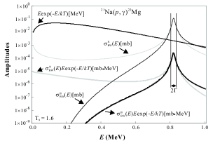
Figure 1: Amplitudes of relevant functions used in the equations. The units are included in the square brackets. See text for details.

2 Validity of Assumptions

The FIRST assumption

Chronically a resonance for which $\Gamma/E_{R}$$<$10 % was treated as a narrow resonance (e.g., see  bib:rol88 ), here it shows this definition of ‘narrow’ is inappropriate especially at low temperatures. If one defines the variation $\delta_{MB}$ of the Maxwell-Boltzmann function $E\mathrm{exp}(-E/kT)$ over the resonance region as

$$\delta_{MB} = 1-\frac{E_{R}+\Gamma/2}{E_{R}}\mathrm{exp}\left(-\frac{E_{R}+\Gamma/2-E_{R}}{kT}\right)$$

$$= 1-\left(1+\frac{\Gamma/2}{E_{R}}\right)\mathrm{exp}\left(-\frac{\Gamma}{2kT}\right),$$

then $\delta_{MB}$ may be large at certain circumstances (e.g., assuming a resonance with $\Gamma$=16 keV and $\frac{\Gamma}{E_{R}}$=10 %, $\delta_{MB}$$\approx$59 %, 17 % at $T$ = 0.1, 0.4 GK, respectively). Clearly, the variation $\delta_{MB}$ exponentially depends on the stellar temperature, and therefore this assumption is not a good one for low temperatures. From the definition of $\delta_{MB}$, another complementary restriction for a narrow resonance should be expressed as $\Gamma\leq\frac{T_{9}}{11.608}\ln\frac{1+\frac{\Gamma/2}{E_{R}}}{1-\delta_{MB}}$ ($\Gamma$ in unit of MeV). For instance, with $\delta_{MB}$=5 % and $\Gamma/E_{R}$$<$10 %, another restriction for width is $\Gamma\leq$ 0.017 $T_{9}$ MeV. It should be noted that in some literature a definition of ‘narrow’ was $\Gamma$$\ll$$E_{R}$, but its ambiguity may give rise to certain misleading in some sense.

The SECOND assumption

The de Broglie wavelength squared $(\frac{\lambda}{2\pi})^{2}$ (=$\frac{\hbar^{2}}{2\mu E}$) is inversely proportional to the center-of-mass energy $E$, and therefore this assumption $(\frac{\lambda}{2\pi})^{2}$$\simeq$$(\frac{\lambda}{2\pi})_{R}^{2}$ means $E$$\simeq$$E_{R}$ over the resonance region. It’s a reasonable assumption for a resonance with $\Gamma/E_{R}$$<$10 %.

The THIRD assumption

The partial width for a charged particle $a$ (usually either proton or $\alpha$-particle) is strongly energy dependent because the projectile must penetrate the Coulomb barrier, and can be defined as (Equ. (4.65) in bib:rol88 )

$$\Gamma_{a}=\frac{2\hbar}{R_{n}}\left(\frac{2E}{u}\right)^{\frac{1}{2}}P_{\ell}\theta^{2}_{\ell},$$

where the penetration factor can be calculated by $P_{\ell}$=$\frac{1}{(F_{\ell}^{2}+G_{\ell}^{2})}$ bib:bar74 with the regular and irregular Coulomb wave functions $F_{\ell}$, $G_{\ell}$. The quantity $\theta^{2}_{\ell}$, called the dimensionless reduced width of a nuclear state, is generally determined experimentally and contains the nuclear structure information. Generally speaking, $\theta^{2}_{\ell}$ is independent of energy $E$. Here, for simplicity, only $s$-wave case has been discussed. Therefore, it is sufficient to use the expression $\Gamma_{a}$=$c_{1}\sqrt{E}P_{\ell=0}(E)$$\propto$$\sqrt{E}e^{-2\pi\eta}$, where the penetration factor $P_{\ell=0}$ for the Coulomb barrier is approximated by a Gamow factor bib:rol88 . The quantity $c_{1}$ depends on the nuclear structure of the resonance. The exponent is $2\pi\eta$=$c_{2}\sqrt{1/E}$ with $c_{2}$=31.29$Z_{1}Z_{2}\sqrt{\mu}$ depending on the projectile-target combination. Note only in this equation the center-of-mass energy $E$ is given in units of keV. On the other hand, $\gamma$-ray partial widths depend only weakly on the energy via $\Gamma_{\gamma}$=$c_{3}E_{\gamma}^{2L+1}$$\propto$$(E+Q)^{2L+1}$, where $E_{\gamma}$ and $L$ are the energy and multipolarity, respectively, of the $\gamma$-ray transition under consideration, and $Q$ is the reaction $Q$-value. The quantity $c_{3}$ depends on the nuclear structure of the two levels involved in the interaction. Therefore, for the usual particle-gamma reaction channel (e.g., $(p,\gamma)$ or $(\alpha,\gamma)$), the variation of quantity $\Gamma_{a}\Gamma_{\gamma}$ ($\propto$$\sqrt{E}(E+Q)^{2L+1}e^{-c_{2}\sqrt{1/E}}$) over the resonance region can be expressed as

$$\delta_{\Gamma_{a}\Gamma_{\gamma}}= \sqrt{1+\Delta E/E_{R}}\times\left(1+\frac{\Delta E}{E_{R}+Q}\right)^{2L+1}$$

$$\times\mathrm{exp}^{-\frac{c_{2}}{\sqrt{E_{R}}}\left(\frac{1}{\sqrt{1+\Delta E/E_{R}}}-1\right)}.$$

Here, $\Delta E$ defines the energy interval between the resonance energy $E_{R}$ and the energies where the Maxwell-Boltzmann function crossing the Breit-Wigner function. It is obvious that the dominate variation takes place in the third exponential term. Given a condition of $\Delta E/E_{R}$ = 5 %, for $p(p,\gamma)$ reaction, $\delta_{\Gamma_{a}\Gamma_{\gamma}}$ are only about 8%, 5%, 4% for resonances at $E_{R}$=0.1, 0.5, 1.0 MeV, respectively; while for ${}^{12}C(p,\gamma)$ reaction, $\delta_{\Gamma_{a}\Gamma_{\gamma}}$ are respectively increased to 58%, 24%, 18% for the above resonance energies. Clearly the variation $\delta_{\Gamma_{a}\Gamma_{\gamma}}$ is very sensitive to the projectile-target combination via quantity $c_{2}$. Therefore, the THIRD assumption is appropriate only for certain projectile-target combinations for a resonance with $\Gamma/E_{R}$$<$10 %.

Actually, the RRR per particle pair for a narrow resonance can be directly written as (use Eqs. 2 & 3)

$$\langle\sigma v\rangle= \sqrt{2\pi}\frac{\hbar^{2}\omega}{(\mu kT)^{3/2}}$$ (7)

$$\times\int^{\infty}_{0}\mathrm{exp}\left(-\frac{E}{kT}\right)\frac{\Gamma_{a}\Gamma_{b}}{(E-E_{R})^{2}+(\Gamma/2)^{2}}dE.$$

If one assumes quantity $\mathrm{exp}(-E/kT)$ as a constant over the resonance region, Equ. 7 is equivalent to Equ. 6. But, obviously this is not a good assumption for certain circumstances (see discussion for the FIRST assumption). As a conclusion, except the SECOND reasonable assumption, the FIRST and THIRD assumptions only hold for certain circumstances.

Now, let’s turn to Equ. 5. Here an approximation (i.e., $\arctan(\frac{E_{R}}{\Gamma/2})$$\simeq$$\frac{\pi}{2}$) was utilized, and hence one can get

$$\int^{\infty}_{0}\frac{1}{(E-E_{R})^{2}+(\Gamma/2)^{2}}dE\simeq\frac{\pi}{\Gamma/2}.$$

This approximation causes about a 3% error for a condition of $\Gamma/E_{R}$= 10%, and thus it can be regarded as a reasonable one. The integration ranges, from 0 to $\infty$, were used in Equ. 5, and therefore the quantity $\Gamma_{a}\Gamma_{b}$ can’t be considered as a constant and taken outside the integral. The quantity $\Gamma_{a}\Gamma_{b}$ can be roughly considered as a constant over a very narrow energy interval, and therefore the integration ranges on Equ. 5 should be physically restricted bib:ang99 . A general equation has been derived here,

$$\int^{E_{R}+n\frac{\Gamma}{2}}_{E_{R}-n\frac{\Gamma}{2}}\frac{1}{(E-E_{R})^{2}+(\Gamma/2)^{2}}dE=\frac{2}{\Gamma/2}\mathrm{arctan}(n).$$ (8)

Ratios between the values of quantity $\frac{\pi}{\Gamma/2}$ and those of quantity $\frac{2}{\Gamma/2}\mathrm{arctan}(n)$ are 0.5, 0.7, 0.8 for $n$=1,2,4, respectively. This effect can be seen in the following Table 1 as well. Thus for a small value of $n$, the ‘look reliable’ derivation of Equ. 5 is inappropriate in the integration-range point of view; while for a large $n$, although the difference becomes small, the above-mentioned assumptions might be inappropriate in the ‘narrow’ point of view. Therefore, the classical analytic Eqs. 4-6 are suggested not to be utilized in the future RRR calculations without caution.

3 Numerical Integration

In the past, some researchers utilized the numerical integration of Equ. 1 with a broad-resonance formula to calculate the resonant-reaction-rate (RRR) of a narrow resonance, while others still utilized the simple analytic expression of Equ. 6. In order to check their differences, as an example, the RRR of a key stellar reaction ²¹Na(p,$\gamma$)²²Mg is discussed below. There is a known resonant state in the compound nucleus ²²Mg at $E_{R}$=0.821 MeV ($J^{\pi}$=$1^{+}$, $\ell$=0) with a proton width of $\Gamma_{p}$=16 keV and a resonant strength of $\omega\gamma$=0.556 eV (here $\Gamma_{\gamma}$$\approx$$\frac{\omega\gamma}{\omega}$=1.48 eV, and hence $\Gamma$$\approx$$\Gamma_{p}$) bib:dau04 . The corresponding $\gamma$-transition to the ground state in ²²Mg is a pure $M$1 transition (i.e., 1⁺$\rightarrow$0⁺) with a multipolarity $L$=1. According to the previous definition, this resonance ($\Gamma/E_{R}$$\simeq$2%) can be ‘reasonably’ treated as a narrow one.

Figure 1 shows the amplitudes of relevant functions used in the equations for this resonance state at the ‘Gamow-peak’ temperature $T$=1.6 GK. The narrow-resonance cross section $\sigma_{BW}^{N}(E)$ is calculated by assuming the constant partial widths $\Gamma_{p}$, $\Gamma_{\gamma}$ (and $\Gamma$). Obviously the tendencies for this cross section and the corresponding integrand curve (indicated by a grey thick solid line) are physically unreal towards lower energies. The reason is the assumption of constant widths is invalid out of the resonance region. If a broad-resonance formula is used in the calculation, the integrand curve (indicated by a thick solid line) become physically reasonable at low energies. Here, the broad-resonance cross section $\sigma_{BW}^{B}(E)$ can be written as, (i.e., Equ. (4.59)) in bib:rol88 ,

$$\sigma(E)_{BW}^{B}=\sigma_{R}\frac{E_{R}}{E}\frac{\Gamma_{p}(E)}{\Gamma_{p}(E_{R})}\frac{\Gamma_{\gamma}(E)}{\Gamma_{\gamma}(E_{R})}\frac{(\Gamma_{R}/2)^{2}}{(E-E_{R})^{2}+[\Gamma(E)/2]^{2}}.$$ (9)

The energy dependence of the proton and $\gamma$-ray partial widths are given by

$$\Gamma_{p}(E)=\Gamma_{p}(E_{R})\frac{P_{\ell=0}(E)}{P_{\ell=0}(E_{R})},$$

$$\Gamma_{\gamma}(E)=\Gamma_{\gamma}(E_{R})B_{\gamma}\left(\frac{E+Q_{p\gamma}-E_{xf}}{E_{R}+Q_{p\gamma}-E_{xf}}\right)^{2L+1},$$

where $Q_{p\gamma}$ is the (p, $\gamma$) reaction $Q$-value ($Q$=5.508 MeV bib:dau04 ), $B_{\gamma}$ is the primary $\gamma$-ray branching ratio to the final state at $E_{xf}$ (Here, $B_{\gamma}$ is assumed to be unity and $E_{xf}$=0 for the ground state). The penetration factors, $P_{\ell}$, are calculated by using a RCWFN bib:bar74 code with a channel-radius parameter of $a_{0}$=1.35 fm.

The numerically and analytically calculated resonant-reaction-rates (RRRs) are compared in Table 1, where the corresponding ratios were listed for different temperatures and integration ranges used in Equ. 7. It can be seen that two methods give almost the same results at ‘Gamow-peak’ temperature $T$=1.6 GK for a full-range integration (0$\rightarrow$$\infty$). For narrow integration ranges, the analytic results are larger than the numerical ones. This shows that the integration should be computed for a full range, and it is not a difficult task anymore with current computers. Notably, at lower temperatures, the numerical results become much larger than the analytic ones (see the 2nd column in Table 1). This implies a higher-energy resonance can contribute to the reaction rate at low temperature significantly (or tremendously) more than the previous analytical result. Furthermore, presume this $E_{R}$=0.821 MeV resonance locating at 0.160, 0.323 MeV, the calculated $Ratio$s for a full-range integration are 0.78, 0.90, respectively, at the relevant ‘Gamow-peak’ temperatures of 0.14, 0.4 GK. This conclusion demonstrates that the previous analytic results may be underestimated by a considerable amount for a resonance with a several keV width even at their ‘Gamow-peak’ temperatures. Although the condition $\Gamma/E_{R}$$<$10 % still holds in these cases, $\delta_{MB}$ varies from 6 % to 37 % for the temperatures listed in Table 1. It indicates that, in the present case, the resonance width is not narrow enough to use the analytic equations at low temperatures, and hence another restriction on the width should be set, e.g., $\Gamma$$\leq$ 3.4 keV for a temperature of 0.2 GK, and it is about five times narrower than the experimental value ($\Gamma$=16 keV).

4 Conclusions

The validity of the resonant-reaction-rate (RRR) equations for an isolated narrow resonance have been reexamined, and it reminds us not to use those analytic equations without careful examination. As a suggestion, it’s better to use the broad-resonance equation to calculate the RRR numerically even for a narrow resonance. In addition, the RRR is usually calculated by using the measured $E_{R}$ and $\omega\gamma$ analytically in the popular direct measurement approach. We think this kind of calculation is inaccurate at low temperatures for a resonance of a few keV width. Because there are still researchers using the analytic equations without rigorous examinations so far, it is worthwhile to address this issue clearly and it will be helpful for the communities. Two years ago, a new book “Nuclear Physics of Stars” bib:iliadis was published, where the definition of a narrow-resonance seems reasonable. But, we should realize that a question is hidden in this sort of calculation, i.e., is it physically appropriate to extend the broad-resonance Breit-Wigner formulism (esp. for a narrow resonance) down to very low energy? since the energy gap between the resonance and the Gamow-peak is quite large, it’s more than hundreds or thousands of resonance width sometimes. However, we can’t address this question in the present work. In addition, some authors bib:ang99 ; bib:iliadis thought that the product of Maxwell-Boltzmann distribution and cross section could give rise to another maximum caused by the low-energy wing of a resonance but, our calculation shows the appearance of this low-energy maximum depends on the temperature condition, for instance, there is no such maximum (but a plateau) in our example beyond $T$$\sim$0.5 GK (of course, no maximum at $T$=1.6 GK in Fig. 1).

Table 1: Ratios of the calculated resonant-reaction-rates (RRRs) using the numerical integration of Equ. 1 with a broad-resonance formula and using the analytic Equ. 6. The ratios are listed for different temperatures and integration ranges, respectively. Additionally the values of $\delta_{MB}$ are listed for different temperatures as well.

	$Ratio=\mathrm{Numerical}/\mathrm{Analytic}$
$T_{9}$(GK)	0 $\rightarrow$ $\infty$	$E_{R}\pm\frac{\Gamma}{2}$	$E_{R}\pm 2\frac{\Gamma}{2}$	$E_{R}\pm 4\frac{\Gamma}{2}$	$\delta_{MB}(\%)$
0.2	2.4$\times 10^{7}$	0.52	0.76	1.02	37
0.4	6.6	0.50	0.72	0.87	21
0.5	1.6	0.50	0.71	0.86	17
1.6	1.0	0.50	0.71	0.84	5.6