Density dependence of valley polarization energy for composite fermions

Abstract

In two-dimensional electron systems confined to wide AlAs quantum wells, composite fermions around the filling factor $\nu=3/2$ are fully spin polarized but possess a valley degree of freedom. Here we measure the energy needed to completely valley polarize these composite fermions as a function of electron density. Comparing our results to the existing theory, we find overall good quantitative agreement, but there is an unexpected trend: The measured composite fermion valley polarization energy, normalized to the Coulomb energy, decreases with decreasing density.

I Introduction

When subjected to high perpendicular magnetic fields, two-dimensional electron systems (2DESs) exhibit a wide variety of exotic phenomena including the fractional quantum Hall effect (FQHE). tsuiPRL82 The composite fermion (CF) theory jainPRL89 ; halperinPRB93 ; CFbook explains the FQHE of electrons by mapping it to the integer QHE of CFs which are electron-magnetic flux quasi-particles. Although absent in the simplest version of the CF theory, the presence of discrete degrees of freedom, such as spin and valley, ushers in a rich variety of phenomena. For many years, understanding the spin polarization of the various FQHE states has been a topic of great interest among experimentalists and theorists alike. In the case of exotic states such as the one formed at Landau level filling factor $\nu=5/2$, the determination of spin-polarization is valuable for deducing the nature of the ground state as its possible non-Abelian statistics has promising consequences for topological quantum computing. nayakRMP08 For other states, e.g. those which form around $\nu=$ 1/2 and 3/2, numerous transport, eisensteinPRL89 ; eisensteinPRB90 ; engelPRB92 ; duPRL95 ; duPRB97 optical, kukushkinPRL99 ; chughtaiPRB02 and nuclear spin resonance and relaxation dementyevPRL99 ; melintePRL00 ; freytagPRL02 ; tracyPRL07 ; liPRL09 studies have aided the understanding of the role of spin in the CF picture. parkPRL98 ; parkSSC01

It was recently shown bishopPRL07 that CFs which form at $\nu=3/2$ in AlAs quantum wells possess a valley degree of freedom which in principle is analogous to spin. In this study, we use in-plane strain to tune the energy of the occupied valleys, and measure the valley splitting energy needed to completely valley polarize the CFs at and around $\nu=3/2$. We find remarkably good agreement between our results and the existing theory which was developed to explain the spin-polarization of CFs in (single-valley) GaAs. parkPRL98 ; parkSSC01 However, the polarization energy, normalized to the Coulomb energy, is found to depend on the 2D electron density ($n$), a feature not explained by the CF theory.

II Experiment details

We report measurements on two samples (A and B) which are 12 and 15 nm-wide AlAs quantum wells grown using molecular beam epitaxy. Details of sample growth are given in Ref. 21. A standard Hall bar is fabricated using photolithography, GeAuNi alloy is used as contact, and metallic front and back gates are deposited on the sample which allow us to control $n$. Studies were done both in a ³He cryostat and a dilution refrigerator at base temperatures of about 0.3 K and $\simeq 50$ mK, respectively and using standard low-frequency lock-in techniques.

III System under study: AlAs

III.1 Effect of strain

The band structure of bulk AlAs has three ellipsoidal conduction band minima (valleys) at the X-points of the Brillouin zone. In quantum wells wider than 5 nm, only two valleys with their major axes lying in the 2D plane are occupied. shayeganPhysicaB06 Their in-plane Fermi contours are anisotropic and are characterized by transverse and longitudinal band effective masses, m_t = 0.205m_e and m_l = 1.05m_e, where m_e is the free electron mass. The degeneracy between these two valleys can be broken by the application of strain which we accomplish by gluing the sample to a piezoelectric stack (piezo), as shown in Fig. 1(a). A voltage $V_{P}$ applied to the piezo induces a strain $\epsilon=\epsilon_{[100]}-\epsilon_{[010]}$ where $\epsilon_{[100]}$ and $\epsilon_{[010]}$ denote strains along the [100] and [010] crystal directions respectively. shayeganPhysicaB06 This strain causes a transfer of electrons from one valley to another. The resulting valley splitting energy is given by $E_{v,e}=\epsilon E_{2}$ where $E_{2}$ is the deformation potential which in AlAs has a band value of 5.8 eV. shayeganPhysicaB06 Although the above picture of valley occupation was first chalked out for the case of electrons, gunawanPRL06 a similar approach for CFs was recently demonstrated. bishopPRL07

III.2 Composite fermion picture around $\nu=3/2$

For the density range under study, the band parameters for AlAs electrons are such that the Zeeman energy is larger than the cyclotron energy. Since there are two valleys available for occupation near $\epsilon=0$, the first two electron Landau levels (LLs) have the same spin. Since the CFs near $\nu=3/2$ form in the second electron LL, this CF system is effectively single-spin and two-valley. This is in contrast to the energy level diagram for GaAs electrons which involves only one valley; however the band parameters in the GaAs system are such that the Zeeman energy is small and the second electron LL is of the opposite spin. Thus, in GaAs, the CFs formed around $\nu=3/2$ form a single-valley, two-spin system. In either case, the CF sea at $\nu=3/2$ is formed by hole-flux composite particles. CFbook These CFs no longer feel the externally applied perpendicular magnetic field, $B$. Instead, they feel an effective magnetic field given by $B_{eff}=3(B-B_{3/2})$ where $B_{3/2}$ is the field at $\nu=3/2$. The various FQHE states formed around $\nu=3/2$ are taken to be the integer QHE states of these CFs. Each fractional electron filling factor ($\nu$) has an integer CF counterpart ($p$). CFbook

IV Results and discussion

In Fig. 1(c) we show magnetoresistance traces for sample A taken at different values of $\epsilon$. At $\epsilon=0$, the FQHE minima at $\nu=5/3$ and 7/5 are very weak or absent while the minimum at $\nu=8/5$ is strong. As we move away from $\epsilon=0$ various minima become weak and strong as a function of $\epsilon$. For example, the traces shown in purple ($\epsilon=0$) and blue ($\epsilon=\pm 0.64\times 10^{-4}$) show the weakest minima for $\nu=7/5$ while those in red ($\epsilon=\pm 0.40\times 10^{-4}$) exhibit the weakest minima for $\nu=8/5$. This behavior can be qualitatively understood by following the simple CF energy fan diagram shown in Fig. 1(b). At $\epsilon=0$ each of the CF LLs is doubly (valley) degenerate. This degeneracy is broken as we apply strain and the two valleys separate in energy. There are specific values of $\epsilon$ at which the LLs of CFs undergo an energetic ”coincidence” thereby causing the gap at the Fermi energy ($E_{F}$) to vanish. For example, the $\nu=7/5$ state (p = 3) is weak at $\epsilon=0$ and undergoes one coincidence as $\epsilon$ increases before becoming completely valley polarized at large $\epsilon$. In transport measurements, these coincidences show up as the weakening of the FQHE minima. At high enough strains all the states become fully valley polarized. Note here that as we apply strain, both the electron and CF LLs split in energy. It is important to realize that in the range of $\epsilon$ depicted in Fig. 1, it is the CFs that become valley polarized; much larger values of $\epsilon$ are needed to valley polarize the $electron$ LLs. bishopPRL07 This two-valley nature of the electron LLs is critical for justifying the description of the CFs as being formed in a ”two-valley, single-spin” system.

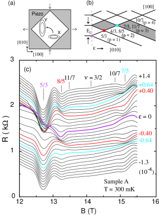
Figure 1: (a) Experimental setup showing the sample glued to a piezo. Schematic transfer of electrons from [100] to [010] valley in response to strain is also shown. (b) Simple energy fan diagram in the CF model for a two-valley, single-spin system. The [100] and [010] valleys are degenerate in energy at $\epsilon=0$ and the degeneracy is lifted as strain is applied. (c) Magnetoresistance traces taken at $T$ = 300mK, at different values of strain (shown on the right in units of $10^{-4}$) for $n=5.1\times 10^{11}$ cm^-2. The traces are offset vertically for clarity.

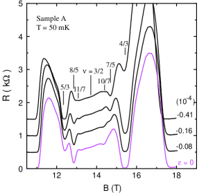
Figure 2: Magnetoresistance traces at $T$ = 50 mK for sample A taken at different values of strain for $n=5.0\times 10^{11}$ cm^-2.

Note that the data in Fig. 1(c) were taken at $T$ = 300 mK. We repeated these measurements at $T=50$ mK in a second cooldown in a different cryostat and the results are shown in Fig. 2. The behavior is qualitatively the same, but we note that resistance minima at some higher order fractions, for example $\nu=11/7$ and 10/7 are better developed.

To demonstrate the response of the various minima to $\epsilon$, we hold $B$ fixed at a particular $\nu$ and sweep $\epsilon$. In Figs. 3(a) and (b), we show results for sample A at $T$ = 300 mK and 50 mK respectively. The peak positions are observed to be temperature independent. Note the symmetry between the positive and negative values of $\epsilon$. This is because the current in this sample is flowing along the [110] crystal direction with respect to which the [100] and [010] valleys are symmetric. In each trace of Fig. 3 the phase and number of oscillations are consistent with the fan diagram in Fig. 1(b). The high quality of this sample is evident from the appearance of higher order fractions (up to $p=4$). The oscillations at the higher order fractions are particularly interesting since the field sweeps show only weak evidence of their existence. Similar measurements in sample B are shown in Fig. 4(a).

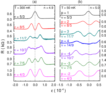
Figure 3: Piezoresistance traces taken for sample A at T = 300 mK (panel (a)) and 50 mK (panel (b)) for different $\nu$. The values of $n$ are given in units of $10^{11}$ cm^-2.

Our piezorsistance data allow us to determine the onset of CF valley polarization at exactly $\nu=3/2$ also. Notice the piezoresistance trace taken at $\nu=3/2$ in Fig. 4(a); for comparison, we also show a trace at $B$ = 0 in Fig. 4(b). The $B$ = 0 trace can be explained qualitatively in a simple model where the conductivities of the two anisotropic valleys add in parallel, leading to an increase in the resistance as the electrons are transferred from one valley to the other. The piezoresistance can also stem from a loss of screening as the electrons become valley polarized and lose their valley degree of freedom; this is analogous to the $magnetoresistance$ exhibited by 2DESs as the electrons become $spin$ polarized in a parallel magnetic field. tutucPRL02 The ”kink” in the piezoresistance and the near-saturation of the resistance at sufficiently large $\epsilon$ signal the full valley polarization of the electrons, gunawanNP07 again, in analogy with the magnetoresistance data. tutucPRL02 Now, as shown in Fig. 4(a), we observe a qualitatively similar behavior at $\nu=3/2$. The resistance at $\nu=3/2$ exhibits a minimum when the two valleys are balanced, increases as the valley degeneracy is broken and saturates once the CFs are fully valley polarized. We take the kink position, marked by an arrow in Fig. 4(a), to signal the complete valley polarization of the CFs. footnote1 We note that very recent experimental data liPRL09 for GaAs CFs at $\nu=1/2$ also show an enhancement, followed by a near-saturation, of the resistance as the CFs become $spin$ polarized.

The energy needed to completely valley polarize the CFs, $E_{v,pol}$, can be obtained directly from Figs. 3 and 4. For $\mid p\mid=2$, 3 and 4, complete polarization is signalled by the outer-most peaks in piezoresistances as these occur at the last coincidence (see e.g., the red square and blue circle in Fig. 1(b)). For the case of $\nu=3/2$, the kink position in the piezoresistance trace is taken as the point of full valley polarization (shown in Fig. 4(a) with an arrow) with the upper and lower excursions included in the error bars. In all cases, $E_{v,pol}=\epsilon_{pol}E_{2}$ where $\epsilon_{pol}$ is the measured threshold strain and $E_{2}$ = 5.8 eV.

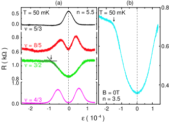
Figure 4: (a) Piezoresistance traces taken for sample B at T = 50 mK for different $\nu$. (b) Piezoresistance for sample B at $B=0$. The values of $n$ are given in units of $10^{11}$ cm^-2.

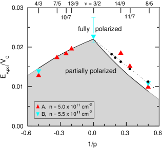
Figure 5: Valley polarization energy in units of Coulomb energy as a function of 1/$p$. Data are shown for both samples at comparable $n$. Theoretical phase boundaries (originally worked out for two-spin system) based on the microscopic CF theory (black circles) and $m_{p}$ model (solid line) from Ref. 18 are also shown.

In Fig. 5 we plot $E_{v,pol}$ for various $\nu$ in units of the Coulomb energy $V_{C}=e^{2}/4\pi\kappa\epsilon_{0}\textit{l}_{B}$ where $\kappa=10$ is the dielectric constant of AlAs and $\textit{l}_{B}=\sqrt{\hbar/eB}$ is the magnetic length. Data from both samples (obtained from Figs. 3(b) and 4(a)) are shown at comparable values of $n$. footnote2 Also shown are small black circles (joined with a dotted line), taken from Ref. 18 which is the theoretical calculation footnote3 using a microscopic CF-wavefunction. Note that the theoretical phase boundary is independent of $n$. This is not surprising since the CF-Hamiltonian comprises entirely of the Coulomb interaction term. Hence all relevant energy scales in the problem should scale as $V_{C}$. Since the calculations are not done for negative values of $p$, we compare our experimental data points to a simpler, one-parameter model which is obtained in Ref. 18 as follows. The points obtained from the microscopic CF theory for positive $p$ are extrapolated to $B_{eff}=0$ (1/$p$ = 0) to obtain an intercept of $E_{v,pol}/V_{C}=0.022$. Since this value corresponds to the complete polarization of the CF sea at $\nu=3/2$, we have $E_{v,pol}=E_{F}=2\pi\hbar^{2}n_{CF}/m_{p}$ which gives $m_{p}=0.47\sqrt{B}$ in units of $m_{e}$. footnote4 $m_{p}$ is defined to be the polarization mass of the CFs. parkPRL98 For a given $p$, the condition of complete polarization can be written as $E_{v}=(p-1)E_{c}$, where $E_{v}$ is the valley splitting of the CFs and $E_{c}=\hbar eB_{eff}/m_{p}$ is the CF cyclotron energy. Using $B_{eff}=3(B-B_{3/2})$ and the fact that $\nu=2-\frac{p}{2p\pm 1}$, the phase boundary can be obtained in terms of $p$ and $m_{p}$. The final result, $E_{v,pol}/V_{C}=0.044\frac{p-1}{2p\pm 1}$, is shown as two solid curves separating the partially- and fully-polarized CFs. Although there is no inherent mass in the CF Hamiltonian, this simple one-parameter model is found to be valuable in interpreting experimental data. parkPRL98 ; parkSSC01

There is overall good agreement between the experimental data points and the theoretical phase boundary, given that there are no adjustable parameters. Not only are the values very close to each other, but also the asymmetry of the phase boundary about $B_{eff}=0$ is reflected in the data. For example, $\nu=4/3$ and 8/5 both correspond to $\mid p\mid=2$. The corresponding values of $E_{v,pol}$, however, are theoretically expected to be different. Consistent with this, our data shows that $E_{v,pol}$ for $\nu=4/3$ is always larger than the value for $\nu=8/5$.

However, this agreement might be fortuitous. First, both the experiment and the theory have errors. Some causes of error in the theoretical calculations for the ideal 2D system are examined in Ref. 18. Our experiment carries an overall uncertainty in the $y$-axis of up to 10$\%$ arising from our strain calibration. Second, and more importantly, the experimental phase boundary for the full valley polarization of CFs depends on $n$, in contrast to the theoretical expectation.

To bring out the $n$-dependence of the phase boundary, we repeated similar measurements for a range of $n$ in both samples and the results are summarized in Fig. 6. The data for sample A were taken at 300 mK (during the first cooldown) and data for sample B at 50 mK. The theoretical predictions based on the single $m_{p}$ model are also shown as dotted lines. Our experimental results show that there is a small, but measurable variation of the normalized polarization energy as a function of $n$. Here we emphasize that, for a given sample, the trend observed as a function of $n$ is unaffected by the $\sim 10\%$ error in our strain gauge calibration.

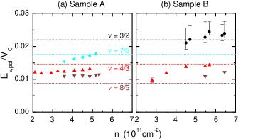
Figure 6: (a) and (b) Valley polarization energy in units of Coulomb energy plotted as a function of $n$ for samples A and B. The dotted horizontal lines are theoretical predictions based on the $m_{p}$ model for the various $\nu$ as indicated. When not shown, error bars are comparable to the symbol size.

The density dependence that emerges from our data demands a better theoretical understanding. Note that residual interactions between CFs cannot be blamed for the trend we observe. This is clear from the $n$-independent nature of the phase boundary obtained from the microscopic CF theory, which in principle includes effects of interaction. parkPRL98 However, Ref. 18 deals with an ideal 2D electron system with no thickness, LL mixing or disorder. In Ref. 19, an attempt was made to address the role of finite layer thickness. A simple way is to replace the bare Coulomb potential $V_{C}=e^{2}/4\pi\kappa\epsilon_{0}\textit{l}_{B}$ with an effective potential $V_{C}^{\prime}=e^{2}/4\pi\kappa\epsilon_{0}\sqrt{l_{B}^{2}+\lambda^{2}}$, where $\lambda$ is the characteristic thickness of the electron wavefunction. In our samples, where electrons are confined to square quantum wells, it is reasonable to assume that $\lambda$ is constant or that it slightly increases with increasing density. Either way, theory expects the value of $E_{v,pol}/V_{C}$ to decrease as a function of increasing $n$, opposite to the trend observed in our experiments. The effects of LL mixing and disorder are unclear at the moment.

- (1) D.C. Tsui, H.L. Stormer, and A.C. Gossard Phys. Rev. Lett. 48, 1559 (1982).
- (2) J.K. Jain, Phys. Rev. Lett. 63, 199 (1989).
- (3) B. I. Halperin, P. A. Lee, and N. Read, Phys. Rev. B 47, 7312 (1993).
- (4) Composite Fermions, Jainendra K. Jain, Cambridge University Press, 2007.
- (5) C. Nayak, S.H. Simon, A. Stern, M. Freedman, and S. Das Sarma, Rev. Mod. Phys. 80, 1083 (2008).
- (6) J.P. Eisenstein, H.L. Stormer, L. Pfeiffer, and K.W. West, Phys. Rev. Lett. 62, 1540 (1989).
- (7) J.P. Eisenstein, H.L. Stormer, L.N. Pfeiffer, and K.W. West, Phys. Rev. B 41, 7910 (1990).
- (8) L.W. Engel, S.W. Hwang, T. Sajoto, D.C. Tsui, and M. Shayegan, Phys. Rev. B 45, 3418 (1992).
- (9) R.R. Du, A.S. Yeh, H.L. Stormer, D.C. Tsui, L.N. Pfeiffer and K.W. West, Phys. Rev. Lett. 75, 3926 (1995).
- (10) R.R. Du, A.S. Yeh, H.L. Stormer, D.C. Tsui, L.N. Pfeiffer and K.W. West, Phys. Rev. B 55, R7351 (1997)
- (11) I.V. Kukushkin, K.v. Klitzing, and K. Eberl, Phys. Rev. Lett. 82, 3665 (1999).
- (12) R. Chughtai, V. Zhitomirsky,R.J. Nicholas, and M. Henini, Phys. Rev. B 65, 161305(R) (2002).
- (13) A.E. Dementyev, N.N. Kuzma, P. Khandelwal, S.E. Barrett, L.N. Pfeiffer, and K.W. West, Phys. Rev. Lett. 83, 5074 (1999).
- (14) S. Melinte, N. Freytag, M. Horvatic, C. Berthier, L.P. Levy, V. Bayot, and M. Shayegan, Phys. Rev. Lett. 84, 354 (2000).
- (15) N. Freytag, M. Horvatic, C. Berthier, M. Shayegan, and L.P. Levy, Phys. Rev. Lett. 89, 246804 (2002).
- (16) L.A. Tracy, J.P. Eisenstein, L.N. Pfeiffer, and K.W. West, Phys. Rev. Lett. 98, 086801 (2007).
- (17) Y.Q. Li, V. Umansky, K. von Klitzing, and J.H. Smet, Phys. Rev. Lett. 102, 046803 (2009).
- (18) K. Park and J.K. Jain, Phys. Rev. Lett. 80, 4237 (1998).
- (19) K. Park and J.K. Jain, Sol. Stat. Commun. 119 291 (2001).
- (20) N.C. Bishop, M. Padmanabhan, K. Vakili, Y.P. Shkolnikov, E.P. De Poortere, and M. Shayegan, Phys. Rev. Lett. 98, 266404 (2007).
- (21) M. Shayegan, E.P. De Poortere, O. Gunawan, Y.P. Shkolnikov, E. Tutuc, and K. Vakili, Phys. Stat. Sol. (b) 243, 3629 (2006).
- (22) O. Gunawan, Y.P. Shkolnikov, K. Vakili, T. Gokmen, E.P. De Poortere, and M. Shayegan, Phys. Rev. Lett. 97, 186404 (2006).
- (23) E. Tutuc, S. Melinte, and M. Shayegan, Phys. Rev. Lett. 88, 036805 (2002).
- (24) O. Gunawan, T. Gokmen, K. Vakili, M. Padmanabhan, E.PḊe Poortere and M. Shayegan, Nature Physics 3, 388 (2007).
- (25) Sample A exhibits a peak instead of saturation near the valley polarization strain at . The cause is unclear, although it might be due to enhanced intervalley scattering near CF valley depopulation, similar to what is seen in 2DESs near subband depopulation [H.L. Stormer, A.C. Gossard and W. Wiegmann, Sol. Stat. Commun. 41 707 (1982)].
- (26) We have data from two other samples including the sample in Ref. 20. The results are consistent with data shown in Fig. 5.
- (27) Although the theory deals with fractions around , it is valid around due to particle-hole symmetry. Also, the theory deals with a two-spin system.
- (28) For GaAs, the corresponding expression is 0.60. The difference in the prefactor is due to the difference in dielectric constants of the host materials, GaAs and AlAs.