See pages - of kasen_ms.pdf

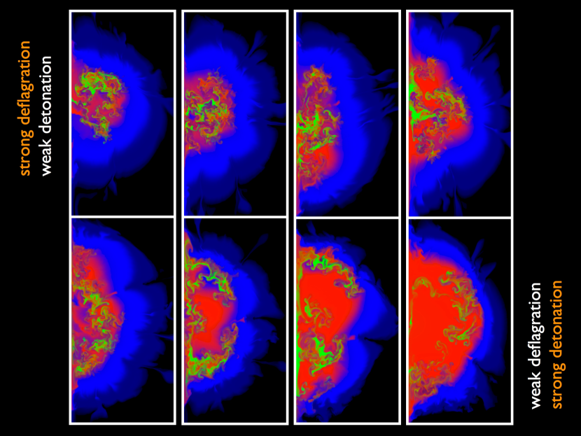
Figure 1: Chemical structure of the ejected debris for a subset of the explosion models. Blue represents intermediate mass elements (i.e., silicon, sulfur, calcium), green stable iron group elements produced by electron capture, and red ${}^{56}\mathrm{Ni}$. The turbulent inner regions reflect Rayleigh-Taylor and other instabilities that develop during the initial deflagration phase of burning. The subsequent detonation wave enhances the ${}^{56}\mathrm{Ni}$ production in the center by burning remaining pockets of fuel. The lower density outer layers of debris, processed only by the detonation, consist of smoothly distributed intermediate mass elements.

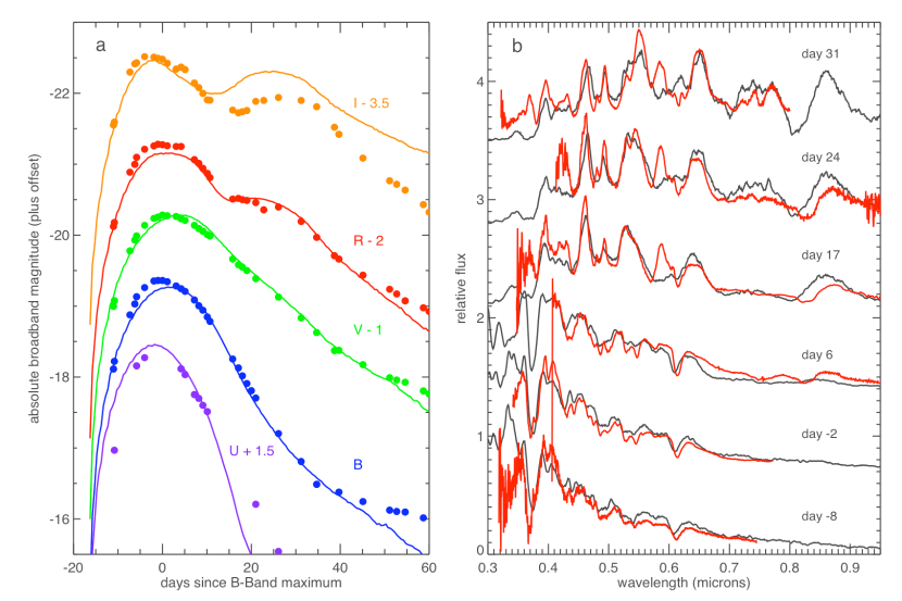
Figure 2: Synthetic multi-color light curves and spectra of a representative explosion model compared to observations of a normal Type Ia supernova. a. The angle-averaged light curves of model DFD_iso_06_dc2 (solid lines) show good agreement with filtered observations of SN 20003du (Stanishev et al., 2007; filled circles) in wavelength bands corresponding to the ultraviolet (U) optical (B,V,R), and near infrared (I). b. The synthetic spectra of the model (black lines) compare well to observations of SN2003du (red lines) taken at times marked in days relative to B light curve maximum. Over time, as the remnant expands and thins, the spectral absorption features reflect the chemical composition of progressively deeper layers of debris, providing a strong test of the predicted compositional stratification of the model.

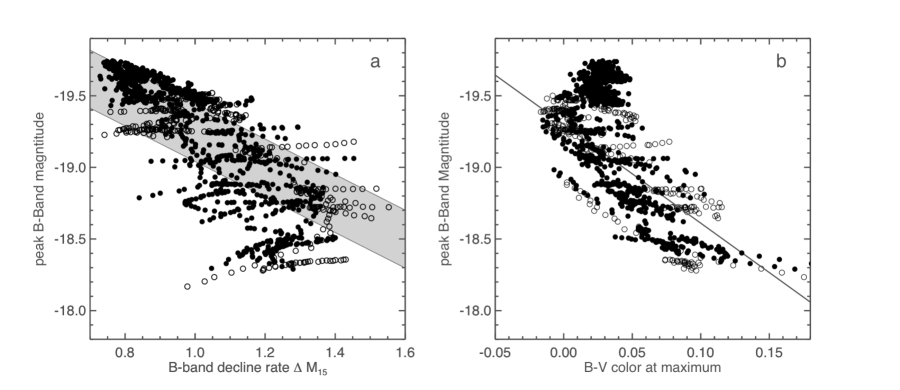
Figure 3: Correlation of the peak brightness of the models with their light curve duration and color. The sample includes 44 models each plotted for 30 different viewing angles. Solid circles denote models computed with the most likely range of detonation criteria, while open circles denote more extreme values. a. Relation between the peak brightness $M_{B}$ (measured in the logarithmic magnitude scale) and the light curve decline rate parameter $\Delta M_{15}$, defined as the decrease in B-band brightness from peak to 15 days after peak. The shaded band shows the approximate slope and spread of the observed width-luminosity relation. b. Relation between $M_{B}$ and the color parameter B-V measured at peak. The solid line shows the slope of the observed relation of Philips et al. (1999) but with the normalization shifted, as the models are systematically redder than observed SNe Ia by  7%, likely due to the approximate treatment of non-LTE effects. In observational studies, these two relations are usually fitted jointly as: $M_{B}=M_{B,0}+\alpha(s-1)+\beta[(B-V)_{\rm Bmax}+(B-V)_{0}]$, where $s$ is a stretch parameter and $(B-V)_{0}$ is the color of a fiducial supernova. We take $(B-V)_{0}=0$ and determine stretch using the first order relation: $s=1-(\Delta M_{15}-1.1)/1.7)$. We find for the models fitted values of $\alpha=2.25,\beta=4.45$ and $M_{B,0}=-19.27$ which are in reasonable agreement with those derived from the recent observational sample of Astier et al. (2006): $\alpha=1.52,\beta=1.57$, and $M_{B,0}=-19.31+5\log_{10}(H_{0}/70)$, where $H_{0}$ is the Hubble parameter.

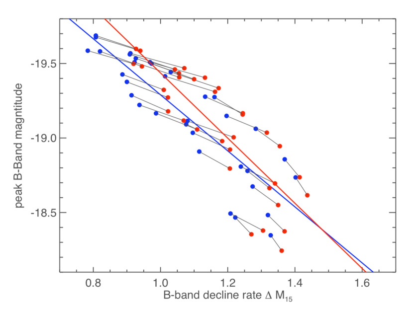
Figure 4: Effect of the metal content of the progenitor star population on the width-luminosity relation. The models explore two extreme values of the metallicity: 3 times (red points) and 0.3 times the solar value (blue points). For clarity, each model has been averaged over all viewing angles, and black lines connect similar explosion models of differing metallicity. The colored lines are linear fits to the width-luminosity relation of of the two metallicity samples separately. The diversity introduced by metallicity variations follows the general width-luminosity trend, but the slightly different normalization and slope of the relation for different metallicity samples indicates a potential source of systematic error in distance determinations.

See pages - of kasen_supplement.pdf