Bose–Einstein condensation and the magnetically ordered state of TlCuCl₃

Abstract

The dimerized $S=\frac{1}{2}$ spins of the Cu²⁺ ions in TlCuCl₃ are ordered antiferromagnetically in the presence of a field larger than about 54 kOe in the zero-temperature limit. Within the mean-field approximation all thermal effects are frozen out below 6 K. Nevertheless, experiments show significant changes of the critical field and the magnetization below this temperature, which reflect the presence of low-energetic dimer-spin excitations. We calculate the dimer-spin correlation functions within a self-consistent random-phase approximation, using as input the effective exchange coupling parameters obtained from the measured excitation spectra. The calculated critical field and magnetization curves exhibit the main features of those measured experimentally, but differ in important respects from the predictions of simplified boson models.

I Introduction

The concept of Bose–Einstein condensation dates back more than 80 years to the prediction of Einstein, based on Bose’s work on the statistics of photons, that a gas of non-interacting massive bosons would condense below a certain critical temperature $T_{c}$. The condensation implies that below $T_{c}$ a non-zero fraction of the total number of particles occupies the lowest single-particle quantum state. For dilute atomic gases this phenomenon was realized experimentally in 1995 for trapped clouds of alkali atoms (see e.g. Ref. HS, ).

For a uniform gas of density $n$ the transition temperature is given by $kT_{c}\approx 3.31\hbar^{2}n^{2/3}/m$, where $m$ is the particle mass. For particles trapped in a harmonic oscillator potential (trap frequencies $\omega_{x}$, $\omega_{y}$ and $\omega_{z}$) one has $kT_{c}\approx 0.94\hbar(N\omega_{x}\omega_{y}\omega_{z})^{1/3}$, where $N$ is the total number of particles. In the latter case the particle mass enters through the trap frequencies, equal to the square root of the force constants in the three directions divided by the particle mass. When a trapped gas is dilute in the sense that the atom–atom scattering length is much less than the interatomic distance, the observed transition temperatures agree well with theoretical expectation for a non-interacting gas. For less dilute gases interaction effects give rise to an observable small shift of $T_{c}$ proportional to the scattering length.

The condensation of massive bosons into a single quantum state is intimately connected to the conservation of particle number. For massless bosons such as phonons or magnons the particle number is not fixed but depends on temperature, and there is therefore no Bose–Einstein condensation in the traditional sense of the term. However, there has been a wide use of model Hamiltonians for magnetic systems that have features in common with those of interacting, massive bosons. The aim of the present work is to consider one such specific system, that of the dimerized Cu²⁺ spins in TlCuCl₃, and compare predictions of such models with calculations that are based on (approximate) solutions of the many-body problem of interacting spins. A recent review of experimental and theoretical developments concerning the magnetic ordering of TlCuCl₃ and related compounds has been given by Giamarchi et al.Giamarchi

Magnetization measurementsOosa99 ; Raffaele and inelastic neutron-scattering experimentsCavadini ; Oosawa demonstrate clearly that nearest-neighboring pairs of $S=\frac{1}{2}$ spins of the Cu²⁺ ions in TlCuCl₃ are dimerized leading to an $S=0$ ground state and an $S=1$ excited triplet around 5.2–5.7 meV above the singlet. Due to the exchange interactions between the dimers the excitations become strongly dispersive, and, in the zero-temperature limit, the minimum energy of the degenerate singlet-triplet mode, at (001), is only about 0.7 meV. When a field is applied, the energy of one of the three normal modes is reduced and goes to zero at a critical field of about 54 kOe at zero temperature. The Cu spins of isostructural KCuCl₃ are similarly dimerized, but the interdimer interactions are relatively weaker and the critical field is about 230 kOe at $T=0$ in this system.OosawaK The phase transition shown by TlCuCl₃ at the field where the excitation energy vanishes, has been analyzed by Nikuni et al.Nikuni They assumed the dimer system to be described by an effective Haniltonian of the form

$${\cal H}=\sum_{{\bm{k}}}\left(\frac{\hbar^{2}k^{2}}{2m}-\mu\right)a_{{\bm{k}}}^{\dagger}a_{{\bm{k}}}^{\phantom{\dagger}}+\frac{v_{0}}{2}\sum_{{\bm{k}},{\bm{k}^{\prime}}\!,{\bm{q}}}a_{{\bm{k}}+{\bm{q}}}^{\dagger}a_{{\bm{k}^{\prime}}-{\bm{q}}}^{\dagger}a_{{\bm{k}^{\prime}}}^{\phantom{\dagger}}a_{{\bm{k}}}^{\phantom{\dagger}}\,,$$ (1)

where the bosonic operators $a^{\dagger}$ and $a$ denote “magnon” creation and annihilation operators and the positive constant $v_{0}$ denotes the strength of the repulsive magnon–magnon interaction, assumed to be a delta function in real space. The quantity $\mu$ plays the role of a chemical potential, assumed proportional to the difference between the applied magnetic field and the critical field. Using $v_{0}$ and $m$ as fitting parameters, Nikuni et al. were able to give a reasonable account of the temperature dependence of the critical field and the magnetization along the applied field in the ordered antiferromagnetic state. An extended version of their theory based on a more realistic dispersion of the magnetic excitations was presented by Misguich and Oshikawa.Misguich However, as we shall see in detail in Sec. IV below, these simplified boson models suffer from inconsistencies that originate in their neglect of the highest level of the triplet. Another, more general problem with boson models is that double occupancy of a local site should be prohibited. In this connection we mention the work of Sirker et al.,Sirker who used a bond-operator approach to map the spin system onto a model of interacting bosons by introducing an infinite on-site repulsion between local triplet excitations.

In the following treatment of the dimerized spin system in TlCuCl₃ we adopt a different point of view and start from the Hamiltonian for the spin system itself, using as input the effective exchange coupling that has been derived from measured excitation spectra. Our approach is a generalization of the zero-temperature theory by Matsumoto et al.,Matsumoto who used the random-phase approximation (RPA) to calculate magnetization curves and excitation spectra for TlCuCl₃. They also considered the case when the phase transition is induced by the application of a hydrostatic pressure.Ruegg2 ; Ruegg08 Here we only address the case of a field-induced transition, but the theory of Matsumoto et al. is extended to include both the effects of quantum fluctuations at zero temperature and the effects of thermal fluctuations. The self-consistent version of the RPA, which is the one applied here, is faced with the similar problem of double occupancy as the boson modelling. However, here this problem is found to have a natural solution by a consideration of the higher order modifications of the Green functions. The self-consistent RPA theory for the paramagnetic phase of the dimer-spin system is presented in Sec. II, which, in Sec. III, is followed by an analysis of the antiferromagnetic phase. A closer examination and discussion of the results obtained are referred to the last Sec. IV.

II Excitations in the paramagnetic phase

II.1 The self-consistent RPA theory

The TlCuCl₃ crystal is monoclinic (space group $P2_{1}/c$) and the lattice parameters are $a=3.9815$ Å, $b=14.144$ Å, $c=8.8904$ Å and $\beta=96.32^{\circ}$ at room temperature.Tanaka The crystal is constructed from layers with configuration Cu₂Cl₆ stacked on top of each other so as to form two chains of Cu ions parallel to the $a$ axis. The chains are separated by Tl ions and pass through the center and corners of the $b$–$c$ plane in the unit cell. There are four Cu ions or two dimer pairs per unit cell. The dimer pair in the unit cell belonging to the chain through a corner is located at site 1: $(x,y,z)$ and site 2: $(\bar{x},\bar{y},\bar{z})$, and the pair belonging to the other chain is placed at site 3: $(x,\bar{y}+\frac{1}{2},z+\frac{1}{2})$ and site 4: $(\bar{x},y+\frac{1}{2},\bar{z}+\frac{1}{2})$. Here $x=0.2338$, $y=0.0486$, and $z=-0.0175$, and the numbering of the sites from 1 to 4 defines the four different Cu-sublattices.

The Hamiltonian is assumed to be

$${\cal H}=-{\textstyle\frac{1}{2}}\sum_{ij}{\cal J}(ij){\bm{s}}_{i}\cdot{\bm{s}}_{j}-g\mu_{B}\sum_{i}{\bm{H}}\cdot{\bm{s}}_{i}\,,$$ (2)

where ${\bm{s}}_{i}$ is the spin-variable of the Cu ion at the $i$th site. The most important exchange parameter is $\Delta=-{\cal J}(i_{1}i_{2})$, where $(i_{1}i_{2})$ are the nearest-neighbor Cu pairs (the 1-2 or the 3-4 ions in the unit cell). The Fourier transform of the Heisenberg exchange interactions between spins on sublattice $\alpha$ and $\beta$ is defined in terms of the remaining coupling parameters

$${\cal J}_{\alpha\beta}({\bm{q}})=\!\!\sum_{j\in\beta\text{-subl.}}^{\prime}\hskip 5.0pt{\cal J}(ij)\,e^{-i{\bm{q}}\cdot({\bm{R}}_{i}-{\bm{R}}_{j})},\quad i\in~{}\alpha\mbox{-subl.},$$ (3)

where ${\bm{R}}_{i}$ is the position of the $i$th dimer, and the prime indicates that the dominating interaction $\Delta$ is excluded from the sum, $(ij)\neq(i_{1}i_{2})$.

When the interactions between the dimers are neglected, the Hamiltonian may be diagonalized exactly in terms of independent products of single-dimer eigenstates. The total spin of the $i$th dimer is ${\bm{S}}_{i}={\bm{s}}_{i_{1}}+{\bm{s}}_{i_{2}}$, where ${\bm{s}}_{i_{1}}$ and ${\bm{s}}_{i_{2}}$ denote the Cu spins belonging to, respectively, the sublattices 1 and 2, or 3 and 4. The total spin defines the basis $|SS_{z}\rangle$, and when the field is along the $z$ axis, the eigenstates of the non-interacting dimer are

• state $|3\rangle=|1-1\rangle$ at the energy $\Delta+h$,

• state $|2\rangle=|10\rangle$ at the energy $\Delta$,

• state $|1\rangle=|1+1\rangle$ at the energy $\Delta-h$,

• state $|0\rangle=|00\rangle$ at zero energy,

with $h=g\mu_{B}|{\bm{H}}|$ and $\Delta$ positive. When $h<\Delta$ the ground state is the non-magnetic singlet $|00\rangle$. In the present section we focus on this condition, and we shall assume that the system stays paramagnetic also in the presence of the interdimer interaction ${\cal J}_{\alpha\beta}({\bm{q}})$. The original Hamiltonian (2) may be rewritten in terms of two dimer-spin variables, the sum ${\bm{S}}_{i}={\bm{s}}_{i_{1}}+{\bm{s}}_{i_{2}}$ and the difference $\bar{\bm{S}}_{i}={\bm{s}}_{i_{1}}-{\bm{s}}_{i_{2}}$. The sum operator only has non-zero matrix elements between the three excited $S=1$ states. We consider the case where the populations of these levels are small (at sufficiently low temperatures in the disordered phase), in which case the dynamical effects due to ${\bm{S}}_{i}$ are negligible. When ${\bm{S}}_{i}$ is neglected, the Hamiltonian involves only a single effective ${\bm{q}}$-dependent exchange term $-\frac{1}{2}\sum_{\bm{q}}J({\bm{q}})\bar{\bm{S}}_{\bm{q}}\cdot\bar{\bm{S}}_{-\bm{q}}$ with

$$J({\bm{q}}) = \frac{1}{4}\left[{\cal J}_{11}({\bm{q}})+{\cal J}_{22}({\bm{q}})-{\cal J}_{12}({\bm{q}})-{\cal J}_{21}({\bm{q}})\right]$$ (4)

$$\pm \frac{1}{4}\left[{\cal J}_{13}({\bm{q}})+{\cal J}_{24}({\bm{q}})-{\cal J}_{14}({\bm{q}})-{\cal J}_{23}({\bm{q}})\right]\,.$$

The presence of two equivalent dimers per unit cell yields two values for the effective interaction for each value of the wave vector within the first Brillouin zone. Alternatively, one may use an extended zone scheme with an effective basis of one dimer per unit cell, in which case only the upper sign applies.

In order to study the spin dynamics of this Hamiltonian we introduce the standard basis operatorsHaley ; Bak ; JJ for the $j$th dimer

$$a_{\mu\nu}^{j}=\left(|\mu\rangle\langle\nu|\right)_{j}\,,\quad\mu,\,\nu=0,\,1,\,2,\,3\,.$$ (5)

In the present case of a dimer system with stationary bonds, these operators serve the same purpose but are of more general use than the “bond operators” applied by Matsumoto et al.Matsumoto In terms of the standard basis operators the components of $\bar{\bm{S}}_{j}$ become

$$\bar{S}_{jx}= \frac{1}{\sqrt{2}}\left[a_{30}^{j}-a_{10}^{j}+a_{03}^{j}-a_{01}^{j}\right],$$ (6)

$$\bar{S}_{jy}= \frac{i}{\sqrt{2}}\left[a_{30}^{j}+a_{10}^{j}-a_{03}^{j}-a_{01}^{j}\right],$$ (7)

$$\bar{S}_{jz}= a_{20}^{j}+a_{02}^{j}\,,$$ (8)

and the Hamiltonian may be written

$${\cal H}=\sum_{i}\left[(\Delta-h)\,a_{11}^{i}+\Delta\,a_{22}^{i}+(\Delta+h)\,a_{33}^{i}\right]\qquad$$ (9)

$$-\sum_{ij}J(ij)\left[a_{01}^{i}a_{10}^{j}+a_{03}^{i}a_{30}^{j}-a_{01}^{i}a_{03}^{j}-a_{10}^{i}a_{30}^{j}\right.$$ (10)

$$+\left.a_{02}^{i}a_{20}^{j}+{\textstyle\frac{1}{2}}\left(a_{20}^{i}a_{20}^{j}+a_{02}^{i}a_{02}^{j}\right)\right],$$ (11)

when only the Fourier transform $J(ij)$ of the effective interaction, Eq. (4), is included. Next we define a $6\times 6$ matrix of Green functionsZubarev

$$\bar{\bar{G}}(ij,\omega)=-\frac{i}{\hbar}\int_{-\infty}^{\infty}\!\!\theta(t)\big{\langle}\big{[}{\bm{a}}_{i}(t),{\bm{a}}_{j}^{\dagger}(0)\big{]}\big{\rangle}e^{i\omega t}dt\,.$$ (12)

A single bracket $\langle\cdots\rangle$ denotes the thermal expectation value, and ${\bm{a}}_{i}(t)$ is a vector operator of site $i$ at time $t$ with components

$${\bm{a}}_{i}=\left(a_{01}^{i},a_{10}^{i},a_{02}^{i},a_{20}^{i},a_{03}^{i},a_{30}^{i}\right).$$ (13)

With the short-hand double-bracket notation $\bar{\bar{G}}(ij,\omega)=\langle\langle{\bm{a}}_{i};{\bm{a}}_{j}^{\dagger}\rangle\rangle$, the equations of motion for the Green functions are (see for instance Ref. JJ, )

$$\hbar\omega\big{\langle}\big{\langle}{\bm{a}}_{i};{\bm{a}}_{j}^{\dagger}\big{\rangle}\big{\rangle}-\big{\langle}\big{\langle}\big{[}{\bm{a}}_{i},{\cal H}\big{]};{\bm{a}}_{j}^{\dagger}\big{\rangle}\big{\rangle}=\big{\langle}\big{[}{\bm{a}}_{i},{\bm{a}}_{j}^{\dagger}\big{]}\big{\rangle}\,,$$ (14)

where the new higher-order Green functions introduced by the second term are determined by the Hamiltonian (9) by the use of the commutator relation

$$\big{[}a_{\mu\nu}^{i},a_{\mu^{\prime}\nu^{\prime}}^{j}\big{]}=\delta_{ij}\left(\delta_{\nu\mu^{\prime}}a_{\mu\nu^{\prime}}^{i}-\delta_{\mu\nu^{\prime}}a_{\mu^{\prime}\nu}^{i}\right)\,.$$ (15)

By using an RPA decoupling of the higher-order Green functions, $a_{\mu\nu}^{i}a_{\mu^{\prime}\nu^{\prime}}^{j}\approx a_{\mu\nu}^{i}\langle a_{\mu^{\prime}\nu^{\prime}}^{j}\rangle+\langle a_{\mu\nu}^{i}\rangle a_{\mu^{\prime}\nu^{\prime}}^{j}$, one finds that the equations of motion are reduced to a closed set of equations, which are solvable by a Fourier transformation. Further, the $6\times 6$ matrix equations decouple into 3 sets of $2\times 2$ matrix equations, and one of these is

$$\left(\begin{matrix}\hbar\omega-E_{1}&-J_{1}\\ J_{3}&\hbar\omega+E_{3}\end{matrix}\right)\left(\begin{matrix}G_{11}&G_{16}\\ G_{61}&G_{66}\end{matrix}\right)=\left(\begin{matrix}n_{01}&0\\ 0&-n_{03}\end{matrix}\right).$$ (16)

The Green functions depend on the Fourier variables, $G_{\mu\nu}=G_{\mu\nu}({\bm{q}},\omega)$, and we have introduced the following parameters

$$E_{1}=\Delta-h-J_{1}\,,\qquad J_{1}=n_{01}J({\bm{q}})\,,$$

$$E_{3}=\Delta+h-J_{3}\,,\qquad J_{3}=n_{03}J({\bm{q}})\,,$$ (17)

with $n_{\mu}$ being the average population of the $\mu$th dimer level

$$n_{\mu}=\langle a_{\mu\mu}^{i}\rangle\,,\quad\mbox{and the difference}\quad n_{\mu\nu}=n_{\mu}-n_{\nu}\,.$$ (18)

Inversion of the first matrix in Eq. (16) results in

$$\left(\begin{matrix}G_{11}&G_{16}\\ G_{61}&G_{66}\end{matrix}\right) = \frac{-1}{(E_{\bm{q}}^{-}-\hbar\omega)(E_{\bm{q}}^{+}+\hbar\omega)}$$

$$\times \left(\begin{matrix}n_{01}(E_{3}+\hbar\omega)&-n_{03}J_{1}\\ -n_{01}J_{3}&n_{03}(E_{1}-\hbar\omega)\end{matrix}\right)\,.$$

The poles of the Green functions determine the excitation energies $E_{\bm{q}}^{\pm}$, which are given by

$$E_{\bm{q}}^{\pm}=E_{\bm{q}}\pm\left(h-{\textstyle\frac{1}{2}}n_{13}J({\bm{q}})\right),$$ (20)

$$E_{\bm{q}}^{2}=\Delta^{2}-(n_{01}+n_{03})\Delta J({\bm{q}})+\left({\textstyle\frac{1}{2}}n_{13}J({\bm{q}})\right)^{2}.$$

The (2,5) part of $\bar{\bar{G}}({\bm{q}},\omega)$ is given by the same expression as the (1,6) part in Eq. (II.1), except that $\omega$ is replaced by $-\omega$. The result for the (3,4) part is that obtained from Eq. (II.1) for $h=0$, corresponding to the replacement of $n_{01}$ and $n_{03}$ by $n_{02}$, and it leads to poles at the energies $\pm E_{\bm{q}}^{z}$, where

$$E_{\bm{q}}^{z}=\sqrt{\Delta^{2}-2\Delta J_{2}}\,,\quad J_{2}=n_{02}J({\bm{q}})\,.$$ (21)

We introduce the following matrix of equal-time correlation functions

$$\bar{\bar{A}}({\bm{q}})=\frac{1}{N}\sum_{ij}\big{\langle}{\bm{a}}_{i}\,{\bm{a}}_{j}^{\dagger}\big{\rangle}\,e^{-i{\bm{q}}\cdot({\bm{R}}_{i}-{\bm{R}}_{j})}\,,$$ (22)

where $N$ is the number of dimers. According to the fluctuation-dissipation theorem (see e.g. Ref. JJ, )

$$\bar{\bar{A}}({\bm{q}})=-\frac{1}{\pi}\int_{-\infty}^{\infty}\frac{1}{1-e^{-\beta\hbar\omega}}\,\bar{\bar{G}}^{\prime\prime}({\bm{q}},\omega)\,d(\hbar\omega)\,,$$ (23)

where $\bar{\bar{G}}^{\prime\prime}$ denotes the imaginary part of the matrix Green function and $\beta=1/kT$. By definition, the average value of, for instance, the $11$-component is

$$\overline{A}_{11}=\frac{1}{N}\sum_{\bm{q}}A_{11}({\bm{q}})=\langle a_{01}^{i}\,a_{10}^{i}\rangle=\langle a_{00}^{i}\rangle=n_{0}\,.$$ (24)

Hence, by calculating the ${\bm{q}}$ averages of the correlation functions, the Green functions may be used for determining the populations of the dimer levels. From the diagonal part of the $\overline{A}$-matrix, we get straightforwardly

$$\frac{n_{0}+n_{1}}{2n_{01}}+\frac{n_{0}+n_{3}}{2n_{03}}\! = \!\frac{1}{N}\sum_{\bm{q}}\frac{E_{1}+E_{3}}{E_{\bm{q}}^{+}+E_{\bm{q}}^{-}}\left(1+n_{\bm{q}}^{-}+n_{\bm{q}}^{+}\right),$$

$$\frac{n_{0}+n_{1}}{2n_{01}}-\frac{n_{0}+n_{3}}{2n_{03}}\! = \!\frac{1}{N}\sum_{\bm{q}}\left(n_{\bm{q}}^{-}-n_{\bm{q}}^{+}\right)$$ (25)

and

$$\frac{n_{0}+n_{2}}{n_{02}}=\frac{1}{N}\sum_{\bm{q}}\frac{\Delta-J_{2}}{E_{\bm{q}}^{z}}\left(1+2n_{\bm{q}}^{z}\right)\,,$$ (26)

where

$$n_{\bm{q}}^{\pm}=\frac{1}{e^{\beta E_{\bm{q}}^{\pm}}-1}\,,\qquad n_{\bm{q}}^{z}=\frac{1}{e^{\beta E_{\bm{q}}^{z}}-1}\,.$$ (27)

The three equations determine the four population numbers, when they are supplemented by the exact condition that

$$n_{0}+n_{1}+n_{2}+n_{3}=1\,.$$ (28)

The RPA decoupling is valid in the mean-field (MF) approximation, where the thermal averages are determined by the Hamiltonian ${\cal H}_{\text{MF}}$ for the non-interacting system, i.e. within the approximation $\langle a_{\mu\nu}\rangle\approx\mbox{Tr}[a_{\mu\nu}\exp(-\beta{\cal H}_{\text{MF}})]=\delta_{\mu\nu}n_{\mu}^{\text{MF}}$. In the case of strong dispersion, this approximation certainly underestimates the populations of the excited levels. Anticipating that the correlation effects predicted by the RPA theory are reasonably trustworthy, the self-consistent equations above should lead to a more accurate determination of the population numbers than that offered by the MF approximation. Unfortunately, the present theory also predicts that the off-diagonal components of the $\overline{A}$ matrix are non-zero contradicting that, for instance, $\overline{A}_{16}=\langle a_{01}^{i}a_{03}^{i}\rangle$ should vanish identically. Phrased differently, this inconsistency implies that the RPA result for the occupation numbers is not unique but depends on the particular choice of correlation functions used in the calculation. A non-zero value of $\langle a_{01}^{i}a_{03}^{i}\rangle$ is the equivalent of a double occupancy of bosons at a single site. Instead of introducing an arbitrary repulsive potential, we are here going to consider possible improvements of the RPA-decoupling procedure applied above.

The present system is in many ways similar to the singlet-doublet system encountered in praseodymium metal. Improvements of the RPA for this system have been derived in Ref. JJPr, , and this theory has been applied to the calculation of the linewidths and the energy renormalization of the excitations in two other dimer systems Cs₂Cr₂Br₉ and KCuCl₃ for the case of zero field.Leu ; CavadiniK It is straightforward to generalize the singlet-doublet theory so as to account for the presence of a third level. Here, we are going to extend the theory to the case where the field is non-zero, and, in the next section, to consider the modifications produced by an ordered moment. The presence of the interdimer interactions $J(ij)$ implies that $a_{00}^{i}$ does not commute with the Hamiltonian. Hence, the assumed ground state, the product state of $|0\rangle_{i}$, is not an eigenstate of the interacting system. The situation compares with the simple Heisenberg antiferromagnet, where the mean-field Néel state is not the true ground state. In this case the RPA theory predicts a zero-temperature reduction of the antiferromagnetic moment from its saturated Néel state value. Equivalently, the RPA results above imply that $n_{0}$ is smaller than its saturation value 1 at zero temperature. The single-dimer population numbers are subject to quantum as well as thermal fluctuations.

One of the terms neglected in the RPA equation (16) involves the Green function $\langle\langle(a_{00}^{i}-a_{11}^{i}-n_{01})a_{01}^{j};{\bf a}_{k}^{\dagger}\rangle\rangle$. Since $a_{00}^{i}$ and $a_{11}^{i}$ are not true constants of motion, this Green function may modify the RPA result. The equations of motion for the Green functions neglected in Eq. (16) have been analyzed in Ref. JJPr, . The consequences are that the RPA parameters are being replaced by effective ones and that the excitations become damped. One of the effective parameters $J_{xy}({\bm{q}})$ replaces $J({\bm{q}})$ in $J_{1}$ and $J_{3}$ in all of the equations above and isJJPr

$$J_{xy}({\bm{q}})=J({\bm{q}})-a_{xy}+\eta_{xy}\left[b_{xy}(\omega)-a_{xy}\right]\,,$$ (29)

where

$$\eta_{xy}=\left(\frac{2}{n_{01}+n_{03}}\right)^{2}-1\,.$$ (30)

The most important modification of $J({\bm{q}})$ is the constant shift introduced by $a_{xy}$, but first we want to discuss the other term

$$b_{xy}(\omega)=\frac{1}{N}\sum_{\bm{k}}\left[J({\bm{k}})\right]^{2}\chi_{xy}({\bm{k},\omega})\,,$$ (31)

where $\chi_{xy}({\bm{k},\omega})$ is a generalized susceptibility.JJPr The imaginary part of $b_{xy}(\omega)$ determines the damping effects, which are, however, small at low temperatures. The renormalization of $J_{xy}({\bm{q}})$ produced by the real part of $b_{xy}(\omega)$ is somewhat smaller than the constant shift due to $a_{xy}$, but it is not entirely negligible. Because of its moderate importance we have simplified the expression for the $b_{xy}(\omega)$ term as follows

$$b_{xy}(\omega) \approx \mbox{Re}\left[b_{xy}(E_{\bm{q}}/\hbar)\right]\approx\left(\frac{n_{01}+n_{03}}{n_{01}^{0}+n_{03}^{0}}\right)^{3}B_{\bm{q}}\,,$$

$$B_{\bm{q}} = \frac{1}{N}\sum_{\bm{k}}\frac{[J({\bm{k}})]^{2}[J({\bm{q}})-J({\bm{k}})]}{[J({\bm{q}})-J({\bm{k}})]^{2}+\epsilon_{0}^{2}}\,.\qquad$$ (32)

We include only the real part and neglect modifications produced by the field. The quantity $\epsilon_{0}$ is due to the finite lifetime of the excitations and we take it to be a constant, $\epsilon_{0}\approx 0.1$ meV at zero temperature and field. The linewidths are going to increase rapidly when the temperature becomes comparable to $\Delta/k$. We have accounted for this effect in a rough manner by scaling the result $B_{\bm{q}}$ at zero temperature and field by the population-dependent factor in front, where $n_{\mu}^{0}$ is the value of a population number at zero field and temperature. A closer examination indicates that this simple scaling accounts for the increase of the linewidths in a reasonable way. The scale factor is unimportant for the analysis of the low temperature properties, but the power of 3 used in this expression ensures that the scale factor times $\eta_{xy}$ vanishes in the high-temperature limit.

Finally, the most important renormalization effect, the constant term $(1+\eta_{xy})a_{xy}$ in $J_{xy}({\bm{q}})$ in Eq. (29), is determined implicitly by

$$\frac{1}{N}\sum_{\bm{q}}\frac{J_{xy}({\bm{q}})}{E_{\bm{q}}^{+}+E_{\bm{q}}^{-}}\left(1+n_{\bm{q}}^{-}+n_{\bm{q}}^{+}\right)=0\,.$$ (33)

The renormalized value of $\overline{A}_{16}$ is equal to this sum over ${\bm{q}}$ times $n_{01}n_{03}$, and since the sum now vanishes, the condition $\langle a_{01}^{i}a_{03}^{i}\rangle=0$ is satisfied. The parameters $J_{1}$ and $J_{3}$ in Eqs. (16)-(20) are replaced by, respectively, $n_{01}J_{xy}({\bm{q}})$ and $n_{03}J_{xy}({\bm{q}})$, and, similarly, $J_{2}$ in Eq. (21) is replaced by $n_{02}J_{z}({\bm{q}})$, where the effective exchange coupling is

$$J_{z}({\bm{q}})=J({\bm{q}})-a_{z}+\eta_{z}\left[b_{z}(\omega)-a_{z}\right]\,.$$ (34)

Here $\eta_{z}=1/n_{02}^{2}-1$ and $b_{z}(\omega)\approx(n_{02}/n_{02}^{0})^{3}B_{\bm{q}}$. The constant term $(1+\eta_{z})a_{z}$ is determined by the condition that $\langle a_{02}^{i}a_{02}^{i}\rangle=0$. Besides the modifications of the exchange couplings, the energy splitting $\Delta$ in $E_{1}$ and $E_{3}$, or in $E_{2}$, is replaced by, respectively,JJPr

$$\Delta_{1}=\Delta_{3}=\Delta+(a_{xy}+a_{z})/2\,,$$

$$\Delta_{2}=\Delta+a_{xy}\,.$$ (35)

The renormalization of the energy-level separations has not much influence on the final calculations, and the small additional modifications derived in Ref. JJPr, might have been neglected. However, the leading order effects of these extra terms are actually included above by assuming $1+\eta_{xy}$ to be a factor $n_{0}+(n_{1}+n_{3})/2$ smaller than derived in Ref. JJPr, , and, similarly, $1+\eta_{z}$ has been divided by $n_{0}+n_{2}$.

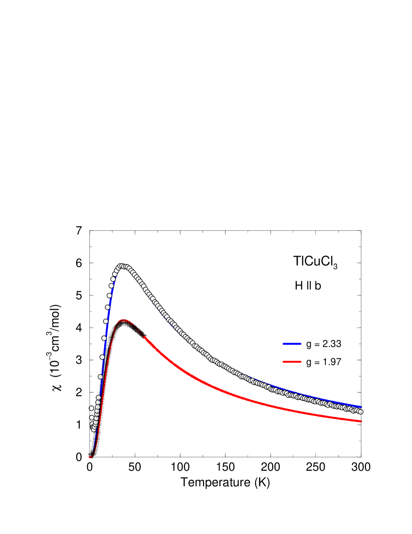
Figure 1: (Color online) The susceptibility of TlCuCl₃ determined experimentally with a field of 10 kOe along the $b$ axis. The pluses show the data of Oosawa et al.,Oosa99 and the open circles are the results of Dell’Amore et al.Raffaele The experimental results are compared with the calculated ones obtained by assuming $g=1.97$ or $g=2.33$. In all other calculations we use $g=2.06$.

II.2 Comparison with experiments

Cavadini et al.Cavadini and Oosawa et al.Oosawa have measured the dispersion of the magnetic excitations in TlCuCl₃ at zero field in the zero-temperature limit (1.5 K). The two sets of results agree where they overlap, and the combined experimental results are most closely reproduced by the dispersion parameters derived by Oosawa et al. The parameters used here (in units of meV) determine the effective exchange coupling according to

$$J_{\text{eff}}({\bm{q}}) = 0.46\cos({\bm{q}}\cdot{\bm{a}})-0.05\cos(2{\bm{q}}\cdot{\bm{a}})$$ (36)

$$+ 1.53\cos\left({\bm{q}}\cdot(2{\bm{a}}+{\bm{c}})\right)$$

$$\mp 0.86\cos\left({\bm{q}}\cdot({\bm{a}}+{\textstyle\frac{1}{2}}{\bm{c}})\right)\cos\left({\textstyle\frac{1}{2}}{\bm{q}}\cdot{\bm{b}}\right)\,.$$

These are the parameters derived by Oosawa et al. except that their coupling between the two chains
$\mp[0.98\cos({\bm{q}}\cdot({\bm{a}}+\frac{1}{2}{\bm{c}}))-0.12\cos(\frac{1}{2}{\bm{q}}\cdot{\bm{c}})]\cos(\frac{1}{2}{\bm{q}}\cdot{\bm{b}})$ has been approximated by a single term. The three modes are degenerate at zero field, and the dispersion relation assumed by Oosawa et al. in their analysis is $E_{\bm{q}}^{2}=\Delta_{\text{eff}}^{2}-2\Delta_{\text{eff}}J_{\text{eff}}({\bm{q}})$ implying that

$$\Delta_{\text{eff}}^{2}=\frac{1}{N}\sum_{\bm{q}}E_{\bf q}^{2}=(\Delta+a_{0})\left(\Delta+a_{0}+2a_{0}/n_{01}^{0}\right),$$

$$J_{\text{eff}}({\bm{q}})=n_{01}^{0}\left[J({\bm{q}})+\eta_{xy}^{0}B_{\bm{q}}\right]\frac{\Delta+a_{0}}{\Delta_{\text{eff}}}\,.$$ (37)

Here $a_{0}$ is the value of $a_{xy}$ or $a_{z}$ at zero temperature and field. The quantity $B_{\bm{q}}$ is roughly proportional to $J({\bm{q}})$ and its averaged value with respect to ${\bm{q}}$ is zero. The RPA equations above have been solved numerically by an iterative procedure. The calculations benefit from the fact that all ${\bm{q}}$ summations may be parameterized in terms of $J_{\text{eff}}({\bm{q}})$ [we neglect the minor difference between $J({\bm{q}})+\eta_{xy}^{0}B_{\bm{q}}$ and $J({\bm{q}})$ in Eq. (II.1) determining $B_{\bm{q}}$]. Hence all summations may be expressed as integrals with respect to $J_{\text{eff}}({\bm{q}})$ times a corresponding “density of states” calculated once and for all from Eq. (36). The value of $\Delta_{\text{eff}}$ used in the calculations is 5.671 meV, (almost) equal to the value of 5.68 meV derived by Oosawa et al.Oosawa Besides this parameter and those defining $J_{\text{eff}}({\bm{q}})$ we have assumed that $g=2.06$, which is the generally accepted value for $g$ in the case where the field is applied along the $b$ axis.Oosa99 ; Raffaele ; Kolezhuk Finally, we have added the mean field from the parallel component to the applied field so that $g\mu_{B}H=h_{0}$ in Eq. (2) is replaced by $h=h_{0}+J_{F}({\bm{0}})\langle S_{z}\rangle$. The ferromagnetic coupling $J_{F}({\bm{0}})$ is estimated to be about $-1.9$ meV by Dell’Amore et al.Raffaele and of the order of $-2.8$ meV by Oosawa et al.Oosawa (using their parameters determined by a cluster series expansion). Here we assume $J_{F}({\bm{0}})=-2.4$ meV. The moment per Cu²⁺ ion parallel to the applied field is

$$m_{z}=\frac{1}{N}\sum_{i}g\mu_{B}\frac{1}{2}\langle S_{iz}\rangle=g\mu_{B}\frac{n_{1}-n_{3}}{2}\,.$$ (38)

It is worthwhile to notice that although the population numbers of the excited levels are predicted to be non-zero at $T=0$, Eq. (II.1)-(28), the quantum fluctuations do not give rise to any difference between $n_{1}$ and $n_{3}$, i.e. $m_{z}=0$ at zero temperature as long as the system stays paramagnetic. This is consistent with the condition that $\sum_{i}S_{iz}=\sum_{i}(a_{11}^{i}-a_{33}^{i})$ commutes with the Hamiltonian.

Using the model defined here we have calculated the susceptibility as a function of temperature. The result is compared with experiments in Fig. 1. The calculated critical field at which the paramagnetic phase becomes unstable is compared with experiments in Fig. 2. The induced magnetic moment $m_{z}$ at various values of the field has been calculated as a function of $T$. These results are shown in Fig. 3. This figure also includes results obtained in the ordered phase, which is considered in the following section.

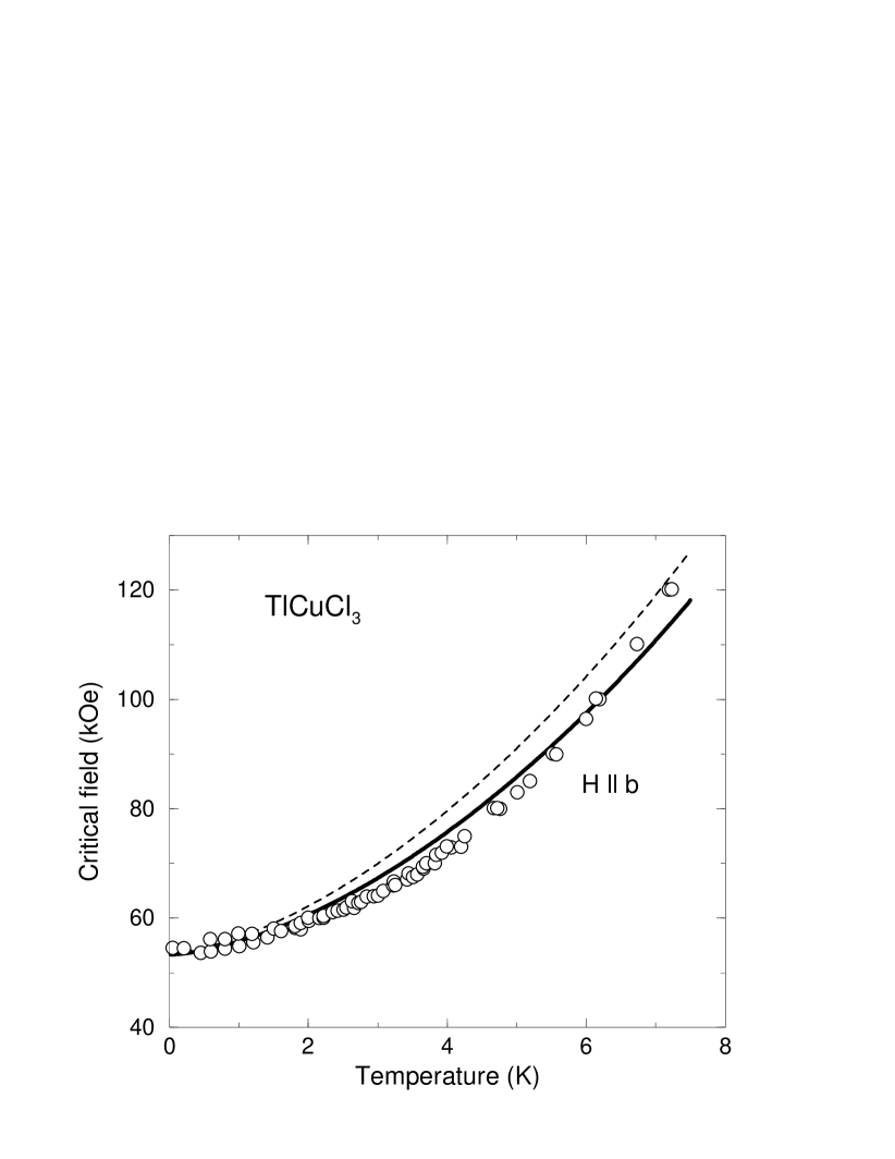
Figure 2: The solid line is the theoretical result for the critical field as a function of temperature using the exchange parameters introduced by Eq. (36). The dashed line is the result obtained if using instead the exchange parameters of Oosawa et al.Oosawa The critical field is here defined to be the one at which the paramagnetic phase becomes unstable. The experimental points are those obtained when the field is applied in the $b$ direction by Oosawa et al.Oosawaheat and Shindo and Tanaka.Shindo

III Excitations in the antiferromagnetic phase

The paramagnetic phase becomes unstable when the energy of the lowest excitation vanishes. The lowest energy mode is the one with the energy $E_{\bm{q}}^{-}$ at ${\bm{q}}={\bm{Q}}=(001)$, and below the transition the expectation value of the dimer-spin variable $\bar{\bm{S}}_{i}$ becomes non-zero. The ordering is antiferromagnetic in the sense that $\langle\bar{\bm{S}}_{i}\rangle$ have opposite signs on the two chain sublattices. The antiferromagnetic ordering may be transformed to the uniform one by an interchange of the two spins in the definition of $\bar{\bm{S}}_{i}$ for the dimers belonging to, for instance, the 3-4 sublattices. The only effect of this transformation is that the interchain coupling between the 1-2 and 3-4 dimers changes sign, i.e. the $\pm$ in front of the second term of $J({\bm{q}})$ in Eq. (4) is being replaced by $\mp$, and $J({\bm{Q}})$ and $J({\bm{0}})$ are being interchanged within the extended zone scheme. That the ordering is antiferromagnetic instead of being uniform does not introduce any further complications. $\langle\bar{\bm{S}}_{i}\rangle$ is perpendicular to the $z$-direction of the field, but its direction within the $x$–$y$ plane is arbitrary (as long as any anisotropy is neglected). For convenience we shall make the choice that the ordered moment is along the $x$ axis, and we define

$$m_{xy}=g\mu_{B}\frac{\langle\bar{S}_{x}\rangle}{2}\,,\qquad\langle\bar{S}_{x}\rangle=\frac{1}{N}\sum_{i}\langle\bar{S}_{ix}\rangle e^{i{\bm{Q}}\cdot{\bm{R}}_{i}}\,.$$ (39)

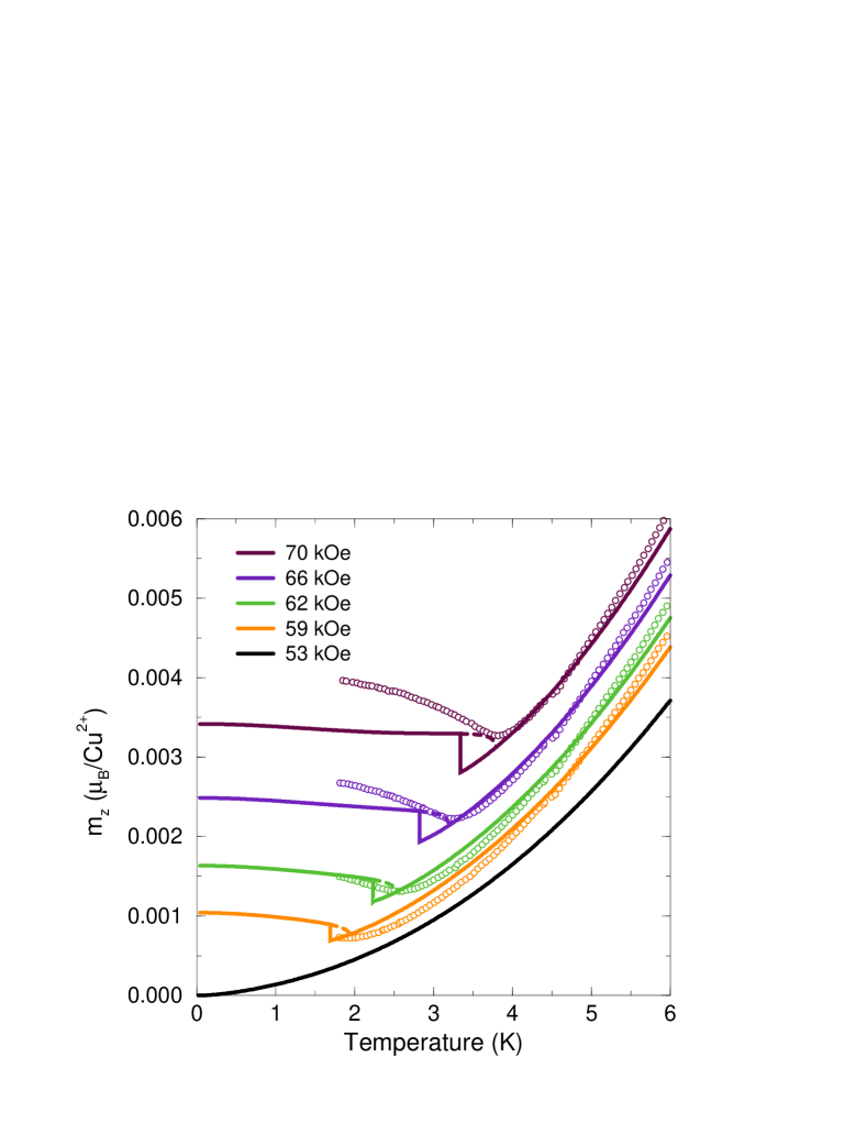
Figure 3: (Color online) The parallel magnetic moment per Cu ion, $m_{z}$, as a function of temperature calculated at various values of the field applied along the $b$ direction. In the case of $H=53$ kOe the system is predicted to stay disordered all the way to zero temperature. The experimental points are a selection of those obtained by Oosawa et al.Oosa99 ; Nikuni

When $\langle\bar{S}_{x}\rangle$ is non-zero, the MF Hamiltonian for the “non-interacting” $i$th dimer becomes

$${\cal H}_{\text{MF}}^{i}=\!\!\!\! (\Delta-h)\,a_{11}^{i}+\Delta\,a_{22}^{i}+(\Delta+h)\,a_{33}^{i}$$ (40)

$$-J({\bm{Q}})\frac{1}{\sqrt{2}}\left[a_{30}^{i}-a_{10}^{i}+a_{03}^{i}-a_{01}^{i}\right]\langle\bar{S}_{x}\rangle$$

in terms of the standard basis operators of the paramagnetic system. We shall continue to label the eigenstates by $|\mu\rangle$, where $\mu=0,1,2,3$, and the ground state of this MF Hamiltonian may then be written

$$|0\rangle=\cos\theta\,|00\rangle-\sin\theta\left[\cos\left(\alpha-{\textstyle\frac{\pi}{4}}\right)\,|1+1\rangle\quad\right.$$

$$+\left.\sin\left(\alpha-{\textstyle\frac{\pi}{4}}\right)\,|1-1\rangle\right]\,.$$ (41)

The two angles $\theta$ and $\alpha$ minimize $\langle 0|{\cal H}_{\text{MF}}^{i}|0\rangle$, or may be determined by demanding the off-diagonal terms of the MF Hamiltonian to vanish, and we get

$$\tan\alpha=\frac{h\cos 2\theta}{\Delta\cos^{2}\theta-h\sin^{2}\theta\sin 2\alpha}$$ (42)

and

$$\sin 2\theta=\frac{2J({\bm{Q}})\cos\alpha}{\Delta\cos 2\alpha}\left(\cos 2\theta+2\sin^{2}\theta\sin^{2}\alpha\right)\langle\bar{S}_{x}\rangle\,.$$ (43)

By calculating the state vectors of the excited MF levels to order $\theta^{2}$, we find that the order parameter is

$$\langle\bar{S}_{x}\rangle=\frac{n_{01}+n_{03}}{2}\sin 2\theta\cos\alpha-n_{13}\sin\theta\sin\alpha+{\cal O}(\theta^{3})\,,$$ (44)

where the higher-order terms ${\cal O}(\theta^{3})$ vanish if $n_{0}=1$, and, likewise, the ferromagnetic component is

$$\langle S_{z}\rangle=n_{13}\cos\theta+\frac{n_{01}+n_{03}}{2}\sin^{2}\theta\sin 2\alpha+{\cal O}(\theta^{4})\,.$$ (45)

By $h_{c}$ we denote the critical field at which these equations have a non-zero solution for $\langle\bar{S}_{x}\rangle$ in the limit of $\theta\to 0$, and this field is found to be determined by

$$1-\left(\frac{h_{c}}{\Delta}\right)^{2}=\frac{J({\bm{Q}})}{\Delta}\left(n_{01}+n_{03}-\frac{h_{c}}{\Delta}\,n_{13}\right)\,.$$ (46)

If we replace $J({\bm{Q}})$ by $J_{xy}({\bm{Q}})$ and $\Delta$ by $\Delta_{1}$ this condition is the same as that derived from the requirement that the energy of the lowest paramagnetic excitation $E_{\bm{Q}}^{-}$, within the self-consistent RPA, should vanish at the transition. The results above are more general but coincide with those derived in the zero-temperature mean-field theory of Matsumoto et al.Matsumoto [Their angle $\phi$ corresponds to our $\frac{\pi}{4}-\alpha$. In our notation $h=h_{0}+J_{F}({\bm{0}})\langle S_{z}\rangle$, whereas in their notation $h$ in Eq. (42) should read $h-J({\bm{Q}})\langle S_{z}\rangle$ corresponding to the replacement of $h_{0}$ by $h$ with their implicit assumption that the ferromagnetic interaction $J_{F}({\bm{0}})$ is equal to $-J({\bm{Q}})$].

When the MF Hamiltonian of the antiferromagnetic phase has been diagonalized we may proceed as in the paramagnetic case for calculating the correlation functions. The positions of the four different levels and the matrix elements of $\bar{\bm{S}}_{i}$ may be calculated analytically if only terms to leading order in $\theta^{2}$ are included. We are not going to present these results, since in the final calculations we chose the more accurate approach of diagonalizing the MF Hamiltonian numerically. In terms of the standard basis operators of the final MF Hamiltonian, $\bar{S}_{jx}$ is now $[m_{3}(a_{30}^{j}+a_{03}^{j})-m_{1}(a_{10}^{j}+a_{01}^{j})]/\sqrt{2}$, where $m_{1}$ and $m_{3}$ are different from 1 and from each other. Here we neglect the extra complication that the matrix elements between the excited states, as for instance $\langle 1|\bar{S}_{jx}|3\rangle\propto\theta$, become non-zero. These excited state contributions to the correlation functions get multiplied by $n_{13}$, hence they are unimportant not only when the ordered moment is small, but in most of the regime where the RPA modifications of the MF behavior are of importance.

The final Hamiltonian may be written in the same way as in the disordered case, Eq. (9). The positions of the three excited levels are being shifted and $J(ij)$ is being multiplied by different factors depending on which operator product is considered, and, finally, the remaining off-diagonal products, $a_{01}^{i}a_{01}^{j}$, $a_{01}^{i}a_{30}^{j}$ etc., now appear. The new off-diagonal contributions are all of order $\theta^{2}$ and affect the diagonal correlation functions only to order $\theta^{4}$. Hence, to leading order these extra contributions may be neglected. In this case the matrix equations once again decouple into 3 sets of $2\times 2$ equations, which may be solved analytically. The result for the population numbers is the same as that given by Eqs. (II.1)-(28), except that $\Delta$ and $\Delta\pm h$ are being replaced by the energies of the three corresponding MF levels and that $J_{1}$, $J_{2}$, and $J_{3}$ are being multiplied by matrix-element factors, which are slightly different from 1 and from each other. The equivalence implies that the modifications of the RPA correlation functions may be calculated as in the paramagnetic case, and, for instance, $a_{xy}$ is still determined by Eq. (33) except that the expressions for $E_{\bm{q}}^{\pm}$ are being modified. We used this approximation, valid in the limit of $\theta^{2}$ being small, for calculating the magnetization curves. The results were close to those shown in Fig. 3, however, in the final calculations we included the higher-order modifications.

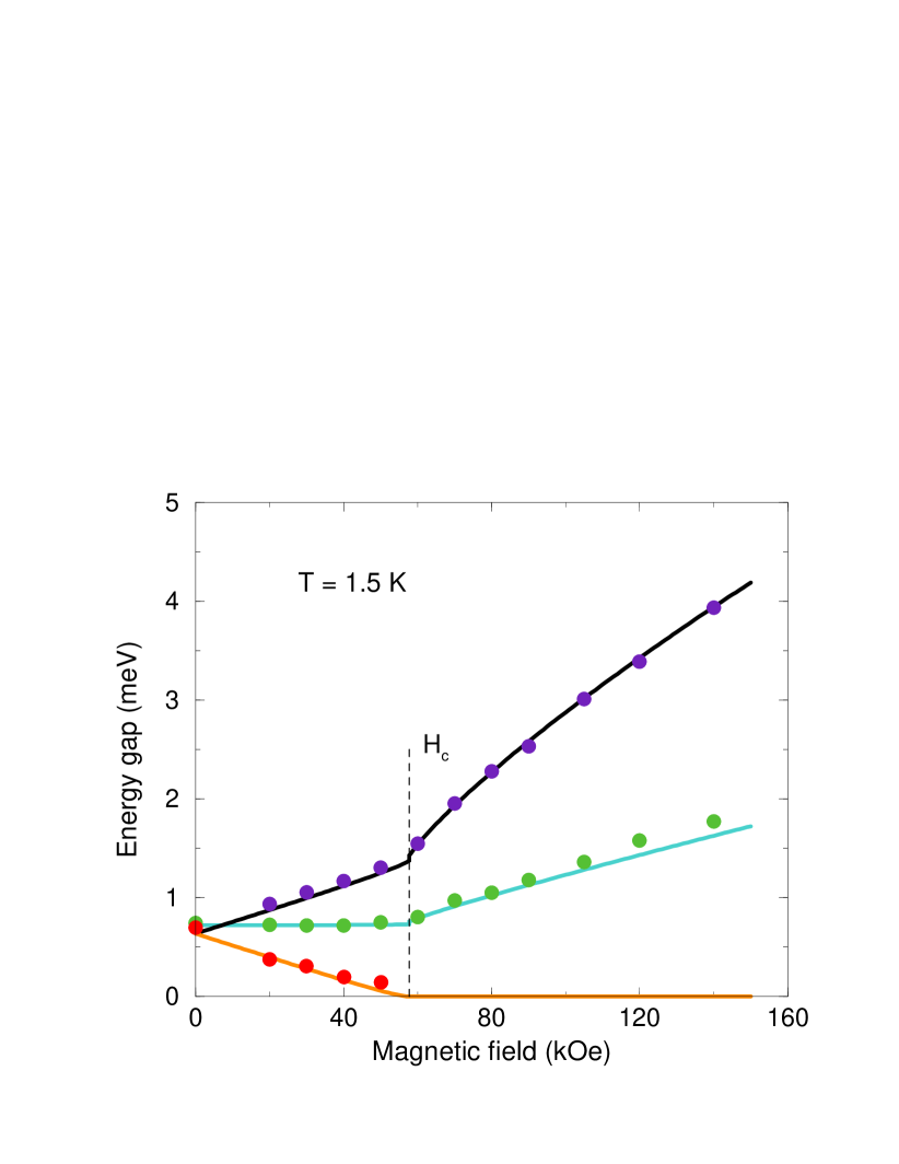
Figure 4: (Color online) The minimum energies of the three different dimer excitations as functions of field at 1.5 K. The calculated results (the solid lines) are compared with the experimental results of Rüegg et al.Ruegg ; RueggN

For a given set of population numbers the MF Hamiltonian was diagonalized numerically, determining all possible matrix elements and the four energy levels. The knowledge of the population numbers and the matrix elements is used for determining the two expectation values $\langle\bar{S}_{x}\rangle$ and $\langle S_{z}\rangle$, and for constructing the total Hamiltonian expressed in terms of the standard basis operators. When the interactions between the excited states are neglected, the equations of motion lead to a $4\times 4$ set of matrix equations for the $xy$ part and a $2\times 2$ set for the longitudinal Green functions. The two sets of equations were inverted analytically (utilizing Mathematica for handling the set of $4\times 4$ equations). In this way we derived an explicit expression for the correlation function matrix $\bar{\bar{A}}({\bm{q}})$. The averaged values of the diagonal components were used for calculating the population numbers as in the paramagnetic case. The renormalization parameter $a_{xy}$ and $a_{z}$ are determined by, respectively, $\overline{A}_{16}=0$ and $\overline{A}_{34}=0$. The condition $\overline{A}_{16}=0$ also implies that $\overline{A}_{25}=0$, but not necessarily that the new off-diagonal components vanish. We have neglected the possibility that the renormalization of the additional off-diagonal exchange terms might be different, since the new terms are small whenever the renormalization effects are important. Except for the matrix-element modification of the exchange terms we use the same approximate expression, Eq. (II.1), for the renormalization parameter $b_{xy}(\omega)$, and similarly for $b_{z}(\omega)$. When the renormalization parameters have been determined we may calculate the renormalized value of $J({\bm{Q}})$ in the MF Hamiltonian (40), which is being replaced by $J_{xy}({\bm{Q}})$ determined from Eq. (30). Similarly $\Delta\pm h$ and $\Delta$ in Eq. (40) are replaced by, respectively, $\Delta_{1}\pm h$ and $\Delta_{2}$ given by Eq. (II.1). The MF Hamiltonian is then consistent with the renormalized RPA expressions, and the whole procedure has been carried out in a self-consistent manner, so that the population numbers assumed as a start are the same as those derived.

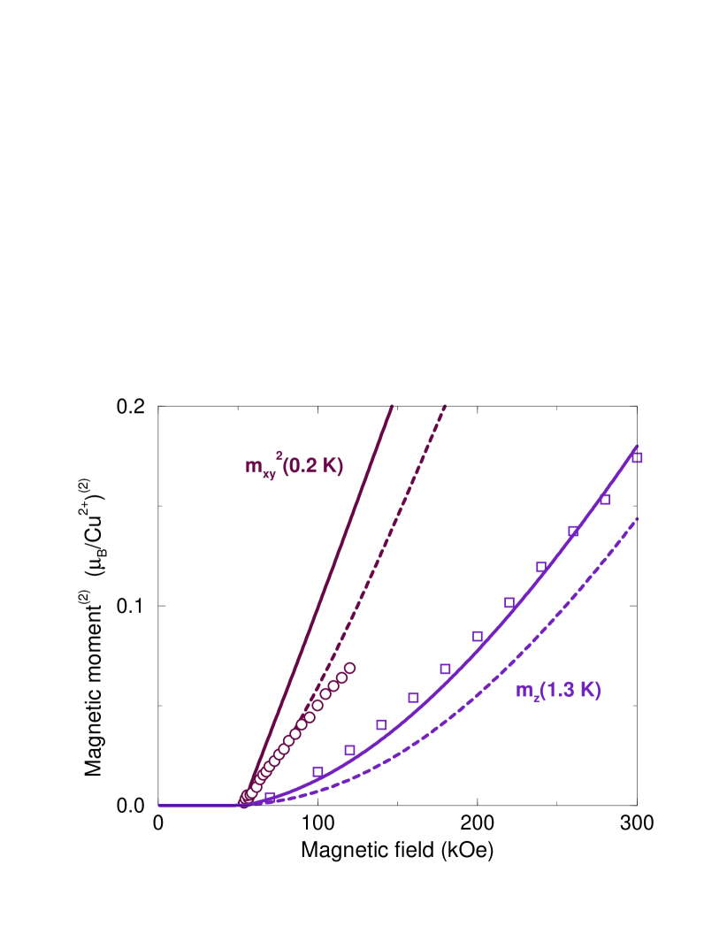
Figure 5: (Color online) The squares are the experimental results for the field dependence of the parallel moment $m_{z}$ at 1.3 K and are the data of Tatani et al.Tatani presented in Ref. Matsumoto, . The open circles are the neutron diffraction results for the square of the ordered antiferromagnetic moment $m_{xy}^{2}$ obtained by Tanaka et al.Tanaka  with the field along the $b$ direction at 0.2 K. The solid lines show the corresponding theoretical predictions, and the dashed ones are the results of using the MF approximation.

This theory was used for calculating the properties of the dimer system in the ordered phase. The temperature dependence of the parallel moment in a constant applied field is shown in Fig. 3. In Fig. 4 we show the calculated energies for the three modes at $(001)$ as functions of field at 1.5 K compared with the neutron-scattering results of Rüegg et al.Ruegg ; RueggN The experimental results indicate that $\Delta$ for the longitudinal mode, the energy of which is nearly unaffected by the field in the paramagnetic phase, is slightly larger than for the two other modes, and we have accounted for this effect by adding 0.03 meV to $\Delta_{2}$ in Eq. (II.1). This modification does not affect the $xy$-polarized modes, and as discussed by Matsumoto et al.,Matsumoto the lowest-energy $xy$-polarized mode becomes the Goldstone mode in the ordered phase, the energy of which depends linearly on $|{\bm{q}}-{\bm{Q}}|$ and is zero at the ordering wave vector.RueggN The spin-resonance experiments of Glazkov et al.Kolezhuk indicate that the Goldstone mode develops an energy gap for fields larger than the critical one corresponding to the presence of a small anisotropy within the $x$–$y$ plane of the same order of magnitude as the anisotropy considered above. The two anisotropy terms are unimportant for the renormalization effects and are neglected elsewhere in the present calculations. The final figure, Fig. 5, shows the field dependencies of the squared primary order parameter $m_{xy}^{2}$ and of the parallel magnetization $m_{z}$ in the zero-temperature limit. The comparison with experiments shows that the self-consistent RPA accounts reasonably well for the field dependence of $m_{z}$, whereas the order parameter is calculated to increase rather faster with field than observed. The corresponding MF model, on the other hand, underestimates the value of $m_{z}$, but predicts an order parameter which is close to the one observed.

IV Discussion

The present dimer system is unique because it clearly exhibits the importance of quantum fluctuations. The system is close to a quantum critical point, and a zero-temperature phase transition may be achieved either by the application of a modest magnetic field of 54 kOeOosa99 or a hydrostatic pressure of 1.1 kbar.Ruegg2 ; Ruegg08 Here we have considered the case where the transition is approached by applying a magnetic field at ambient pressure. The field removes the degeneracy of the $S=1$ triplet states of the dimers, and the collective singlet-triplet excitations separate into a longitudinal, $z$-polarized wave and two transverse modes. The collective transverse modes are linear combinations of propagating modes due to transitions between the ground state and the lowest and the highest excited states of the single dimers. In the paramagnetic phase, the two transverse modes are subject to the same renormalization effects, because the rigid energy shift of the excitations, $E_{\bm{q}}^{+}-E_{\bm{q}}^{-}=2h$, does not influence the quantum fluctuations and $n_{13}=0$ at $T=0$. At non-zero temperatures, the thermal fluctuations imply that $n_{13}$ is non-zero, but the renormalized exchange interaction $J_{xy}({\bm{q}})$ is still the same for the upper and lower transverse modes in the paramagnetic phase (within the present approximation scheme).

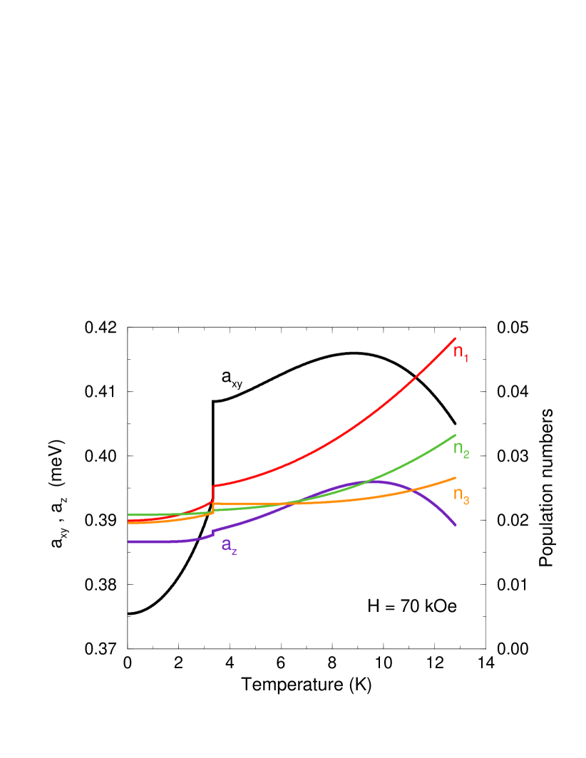
Figure 6: (Color online) The renormalization parameters $a_{xy}$ and $a_{z}$ (left scale) and the population numbers (right scale) calculated as functions of temperature at an applied field of 70 kOe, where the transition occurs at 3.34 K.

The RPA renormalization parameters are determined to be rather substantial in the zero-temperature limit at zero field, because the system is close to the critical point. The occupation number of the dimer ground state is calculated to be $n_{0}^{0}=0.935$ and $a_{0}=0.393$ meV. The constant reduction of the exchange interaction is $(1+\eta_{xy}^{0})a_{0}=0.472$ meV, which is about 17% of the maximum value of the effective exchange interaction $J_{\text{eff}}({\bm{Q}})=2.8$ meV. The effective singlet-triplet splitting is about $\Delta+a_{0}=5.26$ meV in the temperature range of the maximum in the susceptibility. As indicated by the comparison in Fig. 1, this is in good agreement with that derived from the experimental data.Oosa99 ; Raffaele Hence, the theory is able to account for the difference found experimentally between the (effective) energy gap of 5.68 meV, derived from the excitation spectrum in the $T=0$ limit,Oosawa and the smaller value of the gap determined from the susceptibility measurements. At zero temperature the renormalization parameters are independent of the field as long as it stays smaller than the critical one. At non-zero temperature the lower branch $E_{\bm{q}}^{-}$ is much more easily populated than the corresponding MF level. For comparison, the bulk magnetization at 53 kOe predicted by the corresponding MF model is about a factor of 50 times smaller at 6 K. At a constant non-zero temperature $E_{\bm{q}}^{-}$ decreases, and the thermal population of the $E_{\bm{q}}^{-}$-branch increases, when the field approaches the critical one. This also implies that the renormalization parameter $a_{xy}$ increases with increasing field. When the field becomes larger than the critical one, $a_{xy}$ is reduced as the field is further increased. This reduction is so large that it is able to stabilize the ordered moment also at fields smaller than the critical one, i.e. the transition is so strongly modified that it becomes a first order one. This behavior of the renormalization parameters at the phase transition is illustrated in Fig. 6. The unphysical enhancement of the renormalization effects near a phase transition is a quite general feature of the self-consistent version of RPA. In the close neighborhood of the critical point the renormalization effects show a pronounced sensitivity to small modifications of the model, and the rather good agreement between theory and experiments obtained here for the critical field and for the parallel magnetization, see Figs. 2 and 3, is somewhat fortuitous. Even the minor change introduced by using the exchange parameters derived by Oosawa et al.Oosawa rather than those defined by Eq. (36) leads to a relative increase of $a_{xy}$ by about 10% and to corresponding changes of the magnetization curves and the critical field (see Fig. 2).

Focusing our attention on the zero-temperature limit, then $n_{13}$ is zero when the field is smaller than the critical one, but becomes non-zero in the ordered phase. As long as the ordered moment is small, the contributions due to $n_{13}$ may be neglected and the equations determining $\langle\bar{S}_{x}\rangle$ and $\langle S_{z}\rangle$, Eqs. (44) and (45), predict

$$\langle S_{z}\rangle=\frac{h}{\Delta(n_{01}+n_{03})}\langle\bar{S}_{x}\rangle^{2}\,,$$ (47)

when terms of the order of $\theta^{4}$ and $\alpha^{2}\theta^{2}$ are omitted. The equation is only weakly influenced by the renormalization effects since $n_{01}+n_{03}\approx 2$ at $T=0$. Nevertheless, the experimental low-temperature results are far from obeying this relationship, which circumstance makes it difficult to reproduce the field dependencies of the two magnetization components simultaneously, as illustrated by Fig. 5.

In their modelling of the excitations by bosons, Nikuni et al.Nikuni find that $\langle S_{z}\rangle\simeq\frac{1}{2}\langle\bar{S}_{x}\rangle^{2}$ at $T=0$ [in this expression we have neglected the small difference $\tilde{n}$, between $n=\langle S_{z}\rangle$ and $n_{c}$, derived by Nikuni et al., which approximation corresponds to a replacement of $n_{01}+n_{03}$ in Eq. (47) by 2]. Hence, the theory of Nikuni et al. does not include the factor $h/\Delta$ appearing in our relation between $\langle S_{z}\rangle$ and $\langle\bar{S}_{x}\rangle^{2}$. If this factor is included, the results for $m_{xy}$ of Nikuni et al., i.e. $m_{\perp}$ in their Fig. 4, should be multiplied by $\sqrt{\Delta/h}\simeq 2.6$ leading to a slope of $m_{xy}^{2}$ with respect to field, which is nearly twice the one derived by the present theory, i.e. a factor of 3-4 larger than the experimental one (see Fig. 5). In the paramagnetic phase, the lowest excited state of a single dimer is the $|1+1\rangle$ state with $S_{z}=1$, and Nikuni et al. are assuming that this state is the one determining the wave functions of the lowest lying mode of collective excitations, and hence the one which defines the condensate in the ordered phase. This corresponds to assuming $\alpha=\pi/4$ in our Eq. (III). However, as also stressed by Matsumoto et al.,Matsumoto it is crucial to include the presence of the $|1-1\rangle$ level in order to get a consistent description of the excitations and of the condensate. In the paramagnetic phase, the matrix element of $\bar{S}_{x}$ between the ground state $|00\rangle$ and the lowest excited state $|1+1\rangle$ is numerically the same as its matrix element between $|00\rangle$ and $|1-1\rangle$. The same applies to $\bar{S}_{y}$, and this means that the collective transverse excitations transmitted via these two operators are mixed $S_{z}=\pm 1$ excitations. Being proportional to $J({\bm{q}})$, the degree of mixing depends on the wave vector and is at its maximum at the ordering wave vector. In correspondence to this, the MF ground state in the ordered phase, Eq. (III), involves $|1-1\rangle$ as well as $|1+1\rangle$. The two states are of equal importance in the limit of zero field, and the relative weight of the two states is shifted from 1 in the presence of a field as described by the angle $\alpha\simeq h/\Delta$. The two components depend differently on $\alpha$, e.g. $\langle S_{z}\rangle=0$ whereas $\langle\bar{S}_{x}\rangle$ has its maximum at $\alpha=0$, and the factor $h/\Delta$ in Eq. (47) is a simple consequence of this difference.

The present self-consistent RPA theory accounts reasonably well for the paramagnetic properties of the dimer system. Within the MF model, the bulk susceptibility vanishes exponentially in the zero-temperature limit, whereas the present RPA model predicts a power law $m_{z}/H\propto T^{\phi}$ with $\phi=1.8$ at $H=53$ kOe. This is consistent with experiments and the RPA theory also predicts the right critical field for the phase transition. In contrast to the boson model of Eq. (1), the present theory does not rely on any free parameters. Note, however, that if we use the effective exchange parameters, which Oosawa et al. determined from their measurements of the dimer excitation spectrum,Oosawa the critical field is derived to increase slightly faster with temperature than observed, as shown in Fig. 2. This minor discrepancy was neutralized by a small adjustment of the density of states of $J_{\text{eff}}({\bm{q}})$. Actually, it would have been a surprise if the self-consistent RPA theory had been able to predict the right critical field without any adjustments. In all circumstances, it is clear that the theory needs to be corrected due to critical fluctuations, since the self-consistent RPA predicts the phase transition to the antiferromagnetic phase to be of first order in contradiction with experiment.

The dimer system has a number of unusual magnetic properties. The most outstanding one is that the system is driven into the phase of antiferromagnetic order by the application of a uniform field. Another unusual property shown by the ordered phase is that the bulk magnetization increases, when the temperature is lowered at a constant field, as this happens in spite of the fact that the “degrees of freedom” are being reduced because of the accompanying enhancement of the antiferromagnetic order parameter. This behavior is not in accordance with the MF model, whereas the self-consistent RPA theory accounts, at least, qualitatively for this observation. The self-consistent theory of the ordered phase is complicated, and we have been forced to neglect a number of effects. One of the complications, which has not been mentioned above, is that the matrix elements of ${\bm{S}}_{i}$ between the ground state and the excited states are no longer zero in the ordered state implying additional modifications of all normal modes of the system (the two classes of modes may mix because the Cu sites lack inversion symmetry). We may also add that the non-zero values of the diagonal elements of $\bar{S}_{x}$ in the ordered phase effectively give rise to additional contributions to $\Delta_{1}$ and $\Delta_{3}$. Fortunately, these extra complications should be unimportant within the regime of low temperatures and small order parameter, where the theory is applied.

The approximations made for $b_{xy}(\omega)$ in Eq. (II.1) are only acceptable, when the renormalization effects due to this term are small. This term is handled in a more rigorous way by a diagrammatic high-density expansion.Stinch To first order in $1/z$ (where $z$ is the number of interacting neighbors), the diagrammatic theory may be formulated in a self-consistent, “effective medium” fashion, which is the equivalent of the present, self-consistently improved version of RPA.JJ ; JJz This $1/z$ theory has been applied to the Ising systems HoF₃ and LiHoF₄,HoF3 ; LiHoF4 and in these cases the phase transitions are predicted to remain of second order. Therefore, we expect that the use of the $1/z$ expansion theory, to first order in $1/z$, is going to reproduce the self-consistent RPA results derived here for the paramagnetic phase, and should lead to an improved description of the ordered phase.

The present RPA theory establishes a classification of the renormalization effects, which affect the properties of this quantum-critical dimer system. The most important one is the constant reduction of the exchange interaction by $(1+\eta_{xy})a_{xy}$. This term is equivalent to that produced by an on-site repulsive interaction $J_{xy}(ii)$ and is here found to be determined directly from the higher-order modifications of the RPA Green functions. Our analysis of the spin model also predicts the presence of other renormalization effects, such as the $\omega$-dependent correction $b_{xy}(\omega)$ to $J_{xy}({\bm{q}})$ and the increase of the effective splitting between the single-dimer energy levels by $a_{xy}$ or $a_{z}$. The ${\bm{q}}$-independent reduction of the exchange interaction has its parallel in the phenomenological repulsive interaction, $v_{0}$ in Eq. (1), in the boson model of Nikuni et al.,Nikuni whereas the two other renormalization effects have no counterpart in their theory. A more problematic simplification made by Nikuni et al. is their assumption that the low temperature properties of the system are dominated by one type of bosons, whereas, in reality, the system contains three different kinds, where those corresponding to $S_{z}=1$ and $S_{z}=-1$ are mixed. The degree of mixing depends on wave vector and on field, and is important for the characterization of the bosons in the condensate.

One basic difficulty in the many-body theory of localized spin systems is that the operators describing the dynamics of the single spins are not bosonic but more complicated operators, as indicated by Eq. (15). This complication is responsible for the need to renormalize the simple RPA theory. Although the present self-consistent theory includes the leading-order renormalization effects, the comparison between theory and experiments within the ordered phase of TlCuCl₃ is not satisfactory. The diagrammatic $1/z$ theory,Stinch ; JJ ; JJz represents a more systematic approach and should be able to give a more acceptable description of the ordered phase. We expect, however, that the pronounced experimental violation of the MF/RPA relation Eq. (47), between the bulk magnetization and the ordered antiferromagnetic moment, will remain a challenge to future theory.

- (1) C. J. Pethick and H. Smith, Bose–Einstein Condensation in Dilute Gases, Second Edition (Cambridge University Press, Cambridge, 2008).
- (2) T. Giamarchi, Ch. Rüegg, and O. Tchernyshyov, Nature Phys. 4, 198 (2008).
- (3) A. Oosawa, M. Ishii, and H. Tanaka, J. Phys.: Condens. Matter 11, 265 (1999).
- (4) R. Dell’Amore, A. Schilling, and K. Krämer, Phys. Rev. B 78, 224403 (2008).
- (5) N. Cavadini, G. Heigold, W. Henggeler, A. Furrer, H.-U. Güdel, K. Krämer, and H. Mutka, Phys. Rev. B 63, 172414 (2001).
- (6) A. Oosawa, T. Kato, H. Tanaka, K. Kakurai, M. Müller, and H.-J. Mikeska, Phys. Rev. B 65, 094426 (2002).
- (7) A. Oosawa, H. Tanaka, T. Takamasu, H. Abe, N. Tsujii, and G. Kido, Physica B 294-295, 34 (2001).
- (8) T. Nikuni, M. Oshikawa, A. Oosawa, and H. Tanaka, Phys. Rev. Lett. 84, 5868 (2000).
- (9) G. Misguich and M. Oshikawa, J. Phys. Soc. Jpn. 73, 3429 (2004).
- (10) J. Sirker, A. Weisse, and O. P. Sushkov, J. Phys. Soc. Jpn. 74 Suppl., 129 (2005).
- (11) M. Matsumoto, B. Normand, T. M. Rice, and M. Sigrist, Phys. Rev. B 69, 054423 (2004); Phys. Rev. Lett. 89, 077203 (2002).
- (12) Ch. Rüegg, A. Furrer, D. Sheptyakov, Th. Strässle, K. W. Krämer, H.-U. Güdel, and L. Mélési, Phys. Rev. Lett. 93, 257201 (2004).
- (13) Ch. Rüegg, B. Normand, M. Matsumoto, A. Furrer, D. F. McMorrow, K. W. Krämer, H.-U. Güdel, S. N. Gvasaliya, H. Mutka, and M. Boehm, Phys. Rev. Lett. 100, 205701 (2008).
- (14) H. Tanaka, A. Oosawa, T. Kato, H. Uekusa, Y. Ohashi, K. Kakurai, and A. Hoser, J. Phys. Soc. Jpn. 70, 939 (2001).
- (15) S. B. Haley and P. Erdös, Phys. Rev. B 5, 1106 (1972).
- (16) P. Bak, Thesis, Risø Report No. 312 (Risø, Denmark).
- (17) J. Jensen and A. R. Mackintosh, Rare Earth Magnetism: Structures and Excitations (Clarendon Press, Oxford, 1991); http://www.nbi.ku.dk/page40667.htm
- (18) D. N. Zubarev, Usp. Fiz. Nauk 71, 71 (1960) [Sov. Phys.-Usp. 3, 320 (1960)].
- (19) J. Jensen, J. Phys. C: Solid State Phys. 15, 2403 (1982).
- (20) B. Leuenberger and H. U. Güdel, J. Phys. C: Solid State Phys. 18, 1909 (1985).
- (21) N. Cavadini, Ch. Rüegg, W. Henggeler, A. Furrer, H.-U. Güdel, K. Krämer, and H. Mutka, Eur. Phys. J. B 18, 565 (2000).
- (22) V. N. Glazkov, A. I. Smirnov, H. Tanaka, and A. Oosawa, Phys. Rev. B 69, 184410 (2004); A. K. Kolezhuk, V. N. Glazkov, H. Tanaka, and A. Oosawa, Phys. Rev. B 70, 020403(R) (2004).
- (23) A. Oosawa, H. Aruga Katori, and H. Tanaka, Phys. Rev. B 63, 134416 (2001).
- (24) Y. Shindo and H. Tanaka, J. Phys. Soc. Jpn. 73, 2642 (2004).
- (25) Ch. Rüegg, N. Cavadini, A. Furrer, K. Krämer, H. U. Güdel, P. Vorderwisch, and H. Mutka, Appl. Phys. A 74 [Suppl.], S840 (2002).
- (26) Ch. Rüegg, N. Cavadini, A. Furrer, H.-U. Güdel, K. Krämer, H. Mutka, A. Wilders, K. Habicht, and P. Vorderwisch, Nature 423, 62 (2003).
- (27) K. Tatani, K. Kindo, A. Oosawa, and H. Tanaka, (unpublished).
- (28) R. B. Stinchcombe, J. Phys. C: Solid State Phys. 6, 2459 (1973); 6, 2484 (1973).
- (29) J. Jensen, J. Phys. C: Solid State Phys. 17, 5367 (1984).
- (30) J. Jensen, Phys. Rev. B 49, 11833 (1994).
- (31) H. M. Rønnow, J. Jensen, R. Parthasarathy, G. Aeppli, T. F. Rosenbaum, D. F. McMorrow, and C. Kraemer, Phys. Rev. B 75, 054426 (2007).