The Soft Cumulative Constraint

Abstract

This research report presents an extension of Cumulative of Choco constraint solver, which is useful to encode over-constrained cumulative problems. This new global constraint uses sweep and task interval violation-based algorithms.

1 Introduction

The Cumulative global constraint provides a pruning algorithm which takes account of all activities at the same time, which has been proved to be much more efficient than CP approaches considering a conjunction of more primitive constraints. This representation as a global constraint has been widely studied in the literature and integrated into many constraint systems [1, 2, 3, 4, 5].

Definition 1

Let $A=\{a_{1},\ldots,a_{n}\}$ denote a set of $n$ non-preemptive activities. For each $a\in A$,

• $start[a]$ is the variable representing its starting point in time.

• $dur[a]$ is the variable representing its duration.

• $end[a]\in end$ is the variable representing its ending point in time.

• $res[a]$ is the variable representing the discrete amount of resource consumed by $a$, also denoted the height of $a$.

Definition 2

Consider one resource with a limit of capacity $max\_capa$ and a set $A$ of $n$ activities. At each point in time $t$, the cumulated height $h_{t}$ of the set of activities overlapping $t$ is $h_{t}=\sum_{a\in A,start[a]\leq t<end[a]}{min(D(res[a]))}$.

The Cumulative global constraint [1] enforces that:

• C1: For each activity $a\in A,start[a]+dur[a]=end[a]$.

• C2: At each point in time $t$, $h_{t}\leq max\_capa$.

In this research report, we deal with cumulative over-constrained problems that may require to be relaxed w.r.t. the resource capacity at some points in time, to obtain solutions. This motivates the definition of a new global constraint, dedicated to over-constrained instances of problems.

2 Cumulative Constraint with Over-Loads

This section presents the SoftCumulativeSum constraint, useful to express our case-study and deal with significant instances. $D(x)=\{min(D(x)),\ldots,max(D(x))\}$ denotes the domain of variable $x$.

2.1 Pruning Independent from Relaxation

The SoftCumulativeSum constraint that will be presented in section 2.2 implicitly defines a Cumulative constraint with a capacity equal to $max\_capa$. To prune variables in $start$, several existing algorithms for Cumulative can be used. We recall the two filtering techniques currently implemented in the Cumulative of Choco solver [6], which we extend to handle violations in section 2.2.

2.1.1 Sweep Algorithm [4]

The goal is to reduce domains of $start$ variables according to the cumulated profile, which is built from compulsory parts of activities, in order not to exceed $max\_capa$. This is done in Choco using a sweep algorithm [4]. The Compulsory Part [7] of an activity is the minimum resource that will be consumed by this activity, whatever the final value of its start. It is equal to the intersection of the two particular schedules that are the activity scheduled at its latest start and the activity scheduled at its earliest start. As domains of variables get more and more restricted, the compulsory part increases, until it becomes the fixed activity.

Definition 3

The Compulsory Part $CP(a)$ of an activity $a$ is not empty if and only if $max(D(start[a]))<min(D(end[a]))$. If so, its height is equal to $min(D(res[a]))$ on $[max(D(start[a])),min(D(end[a]))[$ and null elsewhere.

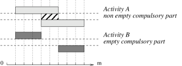
Figure 1: Compulsory parts.

Example 1

Let $a$ be an activity such that $start[a]\in[1,4]$, with a duration fixed to $5$, and $b$ be an activity such that $start[b]\in[1,6]$, with a duration fixed to $3$. As depicted by Figure 1, activity $a$ has a non empty compulsory part, while activity $b$ has an empty compulsory part.

Definition 4

The Cumulated Profile $CumP$ is the minimum cumulated resource consumption, over time, of all the activities. For a given $t$, the height of $CumP$ at time $t$ is equal to

$$\sum_{a\in A/t\in[max(D(start[a])),min(D(end[a]))[}{D(min(res[a]))}$$

That is, the sum of the contributions of all compulsory parts that overlap t.

Next figure shows an example of a cumulative profile $CumP$ where at each point in time $t$ the height of $CumP$ at $t$ does not exceed $max\_capa$.

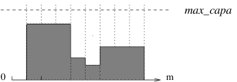
Figure 2: Cumulated profile.

Algorithm

The sweep algorithm moves a vertical line $\Delta$ on the time axis from one event to the next event. In one sweep, it builds the cumulated profile incrementally and prunes activities according to this profile, in order not to exceed $max\_capa$. An event corresponds either to the start or the end of a compulsory part, or to the release date of an activity. All events are initially computed and sorted in increasing order according to their date. Position of $\Delta$ is $\delta$. At each step of the algorithm, a list $ActToPrune$ contains the activities to prune.

• Compulsory part events are used for building $CumP$. All events at date $\delta$ are used to update the height $sum_{h}$ of the current rectangle in $CumP$, by adding the height if it is the start of a compulsory part or removing the height otherwise. The first event with a date strictly greater than $\delta$ gives the end $\delta^{\prime}$ of the current rectangle in $CumP$, finally denoted by $\langle[\delta,\delta^{\prime}[,sum_{h}\rangle$.

• Events corresponding to release dates $d$ such that $\delta\leq d<\delta^{\prime}$ add some new activities to prune, according to $\langle[\delta,\delta^{\prime}[,sum_{h}\rangle$ and $max\_capa$ (those activities which overlap $\langle[\delta,\delta^{\prime}[,sum_{h}\rangle$). They are added to the list $ActToPrune$.

For each $a\in ActToPrune$ that has no compulsory part registered in the rectangle $\langle[\delta,\delta^{\prime}[,sum_{h}\rangle$, if its height is greater than $max\_capa-sum_{h}$ then the algorithm prunes its start times so this activity doesn’t overlap the current rectangle of $CumP$. Then, if the due date of $a$ is less than or equal to $\delta^{\prime}$ then $a$ is removed from $ActToPrune$. After pruning activities, $\delta$ is updated to $\delta^{\prime}$.

Pruning Rule 1

Let $a\in ActToPrune$, which has no compulsory part recorded within the rectangle $\langle[\delta,\delta^{\prime}[,sum_{h}\rangle$. If $sum_{h}+min(D(res[a]))>max\_capa$ then $]\delta-min(D(dur[a])),\delta^{\prime}[$ can be removed from $D(start[a])$.

Time complexity of the sweep technique is $O(n*log(n))$. Please refer to the paper for more details w.r.t. this algorithm [4].

2.1.2 Energy reasoning on Task Intervals [8, 2, 9]

The principle of the energy reasoning is to compare the resource necessarily required by a set of activities within a given interval of points in time with the available resource within this interval. Relevant intervals are obtained from starts and ends of activities (“task intervals”). This section presents the rules implemented in Choco.

Notation 1

Given $a_{i}$ and $a_{j}$ two activities (possibly the same) s.t. $min(D(start[a_{i}]))<max(D(end[a_{j}]))$, we denote by:

• $I_{(a_{i},a_{j})}$ the interval $[min(D(start[a_{i}])),max(D(end[a_{j}]))[$.

• $S_{(a_{i},a_{j})}$ the set of activities whose time-windows intersect $I_{(a_{i},a_{j})}$ and such that their earliest start is in $I_{(a_{i},a_{j})}$, that is, $S_{(a_{i},a_{j})}$ $=$ $\{a\in A$ s.t. $min(D(start[a_{i}]))\leq min(D(start[a]))<max(D(end[a_{j}]))\}$.

• Area${}_{(a_{i},a_{j})}$ the number of free resource units in $I_{(a_{i},a_{j})}$, that is, Area${}_{(a_{i},a_{j})}=(max(D(end[a_{j}]))-min(D(start[a_{i}])))*max\_capa$.

Definition 5

A lower bound $W_{(a_{i},a_{j})}(a)$ of the number of resource units consumed by $a\in S_{(a_{i},a_{j})}$ on $I_{(a_{i},a_{j})}$ is

$$W_{(a_{i},a_{j})}(a)$$

$$=$$

$$min(D(res[a]))$$

$$*$$

$$min[min(D(dur[a])),max(0,max(D(end[a_{j}]))-max(D(start[a])))]$$

Feasibility Rule 1

If $\sum_{a\in S_{(a_{i},a_{j})}}{W_{(a_{i},a_{j})}}(a)>$ Area${}_{(a_{i},a_{j})}$ then fail.

Algorithm

The principle is to browse, by increasing due date, activities $a_{j}\in A$ and for a given $a_{j}$ to browse, by decreasing release date, activities $a_{i}\in A$ such that $\min(D(start[a_{i}]))<\max(D(end[a_{j}]))$. Hence, at each new choice of $a_{i}$ or $a_{j}$ more activities are considered. For each couple $(a_{i},a_{j})$, the algorithm applies the feasibility rule 1.

Suppose the activities sorted by increasing release date i.e. $\min(D(start[a_{1}]))\leq\min(D(start[a_{2}]))\leq\cdots\leq\min(D(start[a_{n}]))$, then:

• If $\min(D(start[a_{i-1}]))=\min(D(start[a_{i}]))$ then
  $S_{(a_{i-1},a_{j})}=S_{(a_{i},a_{j})}$ and therefore $\sum_{a\in S_{(a_{i-1},a_{j})}}{W_{(a_{i-1},a_{j})}}(a)=\sum_{a\in S_{(a_{i},a_{j})}}{W_{(a_{i-1},a_{j})}}(a)$.

• Else
  We have $S_{(a_{i-1},a_{j})}=S_{(a_{i},a_{j})}\cup\{a_{k}\in A,k\leq i-1\wedge\min(D(start[a_{k}]))=\min(D(start[a_{i-1}]))\}$ i.e. we add all activities with same release date than activity $a_{i-1}$. Hence, $\sum_{a\in S_{(a_{i-1},a_{j})}}{W_{(a_{i-1},a_{j})}(a)}=\sum_{a\in S_{(a_{i},a_{j})}}{W_{(a_{i},a_{j})}(a)}+\sum_{\{k\leq i-1\wedge\min(D(start[a_{k}]))=\min(D(start[a_{i-1}]))\}}{W_{(a_{i},a_{j})}(a)}$.

Therefore, the complexity for handling all intervals $I_{(a_{i},a_{j})}$ is $O(n^{2})$.

2.2 Pruning Related to Relaxation

Specific constraints on over-loads exist in real-world applications. To express them, it is mandatory to discretize time, while keeping a reasonable time complexity for pruning. These specific constraints are externalized because they are ad-hoc to each application. On the other hand, the following constraints capture the generic core of this class of problems.

• SoftCumulative extends Cumulative of Choco by maintaining over-loads variables at each point in time, and by pruning activities according to maximal available capacities given by upper bounds of these variables instead of simply considering $max\_capa$. This constraint can be used with various objective criteria.

• The SoftCumulativeSum extends the SoftCumulative. It is defined to deal more efficiently with a particular criterion: minimize the sum of over-loads.

2.2.1 SoftCumulative Constraint

Definition 6

Let A be a set of activities scheduled between time $0$ and $m$, each consuming a positive amount of the resource. SoftCumulative augments Cumulative with a second limit of resource $ideal\_capa\leq max\_capa$, and for each point in time $t<m$ an integer variable $costVar[t]$. It enforces:

• C1 and C2 (see Definition 2).

• C3: For each point in time $t$, $costVar[t]=max(0,h_{t}-ideal\_capa)$

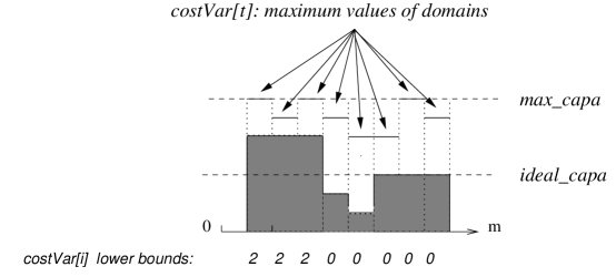
Figure 3: Example of a SoftCumulative constraint.

Example 2

Figure 3 depicts an example of a cumulative profile $CumP$ where at each point in time $t$ the height of $CumP$ at $t$ does not exceed the maximum value in the domain of its corresponding violation variable $costVar[t]$. Time points $1$, $2$, $3$ are such that $CumP$ exceeds $ideal\_capa$ by two. Therefore, for each point, the minimum value of the domain of the correspondong variable in $costVar$ should be updated to value $2$.

Next paragraph details how the classical sweep procedure can be adapted to the SoftCumulative constraint.

Revised Sweep pruning procedure.

The limit of resource is not $max\_capa$ as in the Cumulative constraint. It is mandatory to take into account upper-bounds of variables in $costVar$. One may integrate reductions on upper bounds within the profile, as new fixed activities. However, our discretization of time can be very costly with this method : the number of events may grow significantly. The profile would not be computed only from activities but also from each point in time.

We propose a relaxed version where for each rectangle we consider the maximum $costVar$ upper bound. This entails less pruning but the complexity is amortized: the number of time points checked to obtain maximum $costVar$ upper bounds for the whole profile is $m$, by exploiting the sort on events into the sweep procedure.

Pruning rule 2 reduce domains of start variables from the current maximum allowed over-load in a rectangle.

Pruning Rule 2

Let $a\in ActToPrune$, which has no compulsory part recorded within the current rectangle. If $sum_{h}+min(D(res[a]))>ideal\_capa+max_{t\in[\delta,\delta^{\prime}[}(max(D(costVar[t])))$ then $]\delta-min(D(dur[a])),\delta^{\prime}[$ can be removed from $D(start[a])$.

Proof: For any activity which overlaps the rectangle, the maximum capacity is upper-bounded by $ideal\_capa+max(D(costVar[t]),t\in[\delta,\delta^{\prime}[)$.

Time complexity is $O(n*log(n)+m)$, where $m$ is the maximum due date.

Revised task Intervals energy reasoning.

This paragraph describes the extension of the principle of section 2.1.2 to the SoftCumulative global constraint.

Feasibility Rule 2

Area${}_{(a_{i},a_{j})}=$

$$\sum_{t\in[min(D(start[a_{i}])),max(D(end[a_{j}]))[}ideal\_capa+max(D(costVar[t]))$$

If $\sum_{a\in S_{(a_{i},a_{j})}}{W_{(a_{i},a_{j})}}(a)>$ Area${}_{(a_{i},a_{j})}$ then fail.

Proof: At each time point $t$ there is $ideal\_capa+max(D(costVar[t]))$ available units.

Efficiency of rule 1 can be improved by this new computation of Area${}_{(a_{i},a_{j})}$ (the previous value was an over-estimation). Since activities $a_{i}$ are considered by decreasing release date, it is possible to compute incrementally Area${}_{(a_{i},a_{j})}$. Each upper bound of a variable in $costVar$ are considered once for each $a_{j}$. Time complexity is $O(n^{2}+n*m)$, where $m$ is the maximum due date.

Next paragraph explains how minimum values of domains of variables in $costVar$ are updated during the search process.

Update costVar lower-bounds.

Update of $costVar$ lower bounds can be directly performed within the sweep algorithm, while the profile is computed.

Pruning Rule 3

Consider the current rectangle in the profile, $[\delta,\delta^{\prime}[$. For each $t\in[\delta,\delta^{\prime}[$, if $sum_{h}-ideal\_capa>min(D(costVar[t]))$ then $[min(D(costVar[t])),sum_{h}-ideal\_capa[$ can be removed from $D(costVar[t])$.

Proof: From Definitions 3 and 4.

Usually the constraint should not be associated with a search heuristic that forces to assign to a given variable in $costVar$ a value which is greater than the current lower bound of its domain. Indeed, such a search strategy would consist of imposing at this point in time a violation although solutions with lower over-loads at this point in time exist (or even solutions with no over-load). However, it is required to take into account this eventuality and to ensure that our constraint is valid with any search heuristic. If a greater value is fixed to a variable in $costVar$, until more than a very few number of unfixed activities exist, few deductions can be made in terms of pruning and they may be costly (for a quite useless feature). Therefore, we implemented a check procedure that fails when all start variables are fixed and one variable in $costVar$ is higher than the current profile at this point in time. This guarantees that ground solutions will satisfy the constraint in any case, with a constant time complexity.

2.2.2 SoftCumulativeSum Constraint

Definition 7

SoftCumulativeSum augments SoftCumulative with an integer variable $cost$. It enforces:

• C1 and C2 (see Definition 2), and C3 (see Definition 6).

• The following constraint: $cost~{}~{}=\sum_{t\in\{0,\ldots,m-1\}}costVar[t]$

Pruning procedures and consistency checks of SoftCumulative remain valid for SoftCumulativeSum. Additionally, we aim at dealing with the sum constraint efficiently by exploiting the semantics. We compute lower bounds of the sum expressed by $cost$ variable. Classical back-propagation of this variable can be additionally performed as if the sum constraint was defined separately.

Example 3

The term back-propagation is used to recall that propagation of events is not only performed from the decision variables to the objective variable but also from the objective variable to decision variables. For instance, let $x_{1},x_{2}$ and $x_{3}$ be $3$ variables with the same domain: $\forall i\in\{1,2,3\},D(x_{i})=\{1,2,3\}$. Let $sum$ be a variable, $D(sum)=\{3,4,\ldots,9\}$, and the following constraint $sum=\sum_{i\in\{1,2,3\}}x_{i}$. Assume that $2$ is removed from all $D(x_{i})$. The usual propagation removes values $4$, $6$ and $8$ from $D(sum)$. Assume now that all values greater than or equal to $5$ are removed from $D(sum)$. Back-propagation removes value $3$ from all $D(x_{i})$.

Sweep based global lower bound.

Within our global constraint, a lower bound for the $cost$ variable is directly given by summing the lower bounds of all variables in $costVar$, which are obtained by pruning rule 3. These minimum values of domains were computed from compulsory parts, not only from fixed activities.

$$LB_{1}=\sum_{t\in\{0,\ldots,m-1\}}min(D(costVar[t]))$$

$LB_{1}$ can be computed with no increase in complexity within the sweep algorithm.

Interval based global lower bound.

The quantity $\sum_{a\in S_{(a_{i},a_{j})}}{W_{(a_{i},a_{j})}}(a)$ used in feasibility rule 1 provides the required energy for activities in the interval $I_{(a_{i},a_{j})}$. This quantity may exceed the number of time points in $I_{(a_{i},a_{j})}$ multiplied by $ideal\_capa$. We can improve $LB_{1}$, provided we remove from the computation over-loads yet taken into account in the $cost$ variable. In our implementation, we first update variables in $costVar$ (by rule 3), and compute $LB_{1}$ to update $cost$. In this way, no additional incremental data structure is required.

To obtain the new lower bound we need to compute lower-bounds of $cost$ which are local to each interval $I_{(a_{i},a_{j})}$.

Definition 8

$lb_{1(a_{i},a_{j})}=\sum_{t\in I_{(a_{i},a_{j})}}min(D(costVar[t]))$

Then, next proposition is related to the free available number of resource units within a given interval.

Proposition 1

The number FreeArea${}_{(a_{i},a_{j})}$ of free resource units in $I_{(a_{i},a_{j})}$ s. t. no violation is entailed is $(max(D(end[a_{j}]))-min(D(start[a_{i}])))*ideal\_capa$.

Proof: From Definition 7.

From Definition 8 and Proposition 1, FreeArea${}_{(a_{i},a_{j})}+lb_{1(a_{i},a_{j})}$ is the number of time units that can be used without creating any new over-load into the interval $I_{(a_{i},a_{j})}$ compared with over-loads yet taken into account in $lb_{1(a_{i},a_{j})}$.

Definition 9

Inc${}_{(a_{i},a_{j})}=\sum_{a\in S_{(a_{i},a_{j})}}{W_{(a_{i},a_{j})}}(a)-$FreeArea${}_{(a_{i},a_{j})}-lb_{1(a_{i},a_{j})}$

Inc${}_{(a_{i},a_{j})}$ is the difference between the required energy and this quantity. Even if one variable in $costVar$ has a current lower bound higher that the value obtained from the profile, the increase Inc${}_{(a_{i},a_{j})}$ is valid (smaller, see Definition 8). We are now able to improve $LB_{1}$.

$LB_{2}=LB_{1}+max_{(a_{i},a_{j})\in A^{2}}($Inc${}_{(a_{i},a_{j})})$

Another lower bound can be computed from a partition $P$ of $[0,m[$ in disjoint intervals obtained from pairs of activities $(a_{i},a_{j})$: $LB_{(P)}=LB_{1}+\sum_{I_{(a_{i},a_{j})}\in P}$ Inc${}_{(a_{i},a_{j})}$. Obviousy $LB_{2}\leq LB_{(P)}$. However, time complexity of the algorithm deduced from rule 2 in the SoftCumulative constraint is $O(n^{2}+n*m)$. This complexity should reasonably not be increased. Computing $LB_{2}$ can be directly performed into this algorithm without any increase in complexity.

Pruning Rule 4

If $LB_{2}>min(D(cost))$ then $[min(D(cost)),LB_{2}[$ can be removed from $D(cost)$.

Proof: From Definition 7, $LB_{1}$ is a lower bound of $cost$. Since intervals are disjoint, by Definition 9 the quantity $LB_{(P)}$ is a lower bound of $cost$. $LB_{2}\leq LB_{(P)}$. Therefore $LB_{2}$ is a lower bound of $cost$. The pruning rule holds.

Aggregating local violations.

Once the profile is computed, if some activities having a null compulsory part cannot be scheduled without creating new over-loads, then $LB_{1}$ can be augmented with the sum of minimum increase of each activity. This idea is inspired from generic solving methods for over-constrained CSPs, e.g., Max-CSP [10]. Our experiments shown that there is quite often a way to place any activity without creating a new violation. This entails a null lower bound. Therefore, we removed that computation from our implementation. We inform the reader that we described the procedure in a preliminary technical report [11].

2.2.3 Implementation

Constraints were implemented to work with non fixed durations and resource consumptions.

Instance	$cost$ value	SoftCumulative	SoftCumulativeSum
		+ external sum
1	0	92 (0.07 s)	92 (0.01 s)
2	2	417 (0.29 s)	94 (0.01 s)
3	10	$>$ 30 s	63 (0.01 s)
4	2	1301 (0.59 s)	194 (0.06 s)
5	6	19506 (13.448 s)	97 (0.01 s)
6	0	53 (0.00 s)	53 (0.00 s)
7	10	$>$ 30 s	90 (0.01 s)
8	6	$>$ 30 s	152 (0.07 s)

Table 1: Number of nodes of optimum schedules with $n=9$, $m=9$, durations between $1$ and $4$, resource consumption between $1$ and $3$, $ideal\_capa=3$, $max\_capa=7$.

Table 1 compares the two constraints on small problems when the objective is to minimize $cost$. Results show the main importance of $LB_{2}$ when minimizing $cost$.

3 Extension

The global constraint presented in this research report can be tailored to be suited to some other classes of applications. If the time unit is tiny compared with the makespan, e.g., one minute in a one-year schedule, the same kind of model may be used by grouping time points. For example, each violation variable may correspond to one half-day. Imposing a side constraint between two particular minutes into a one-year schedule is generally not useful. For this purpose, the SoftCumulative constraint can be generalized, to be relaxed with respect to its number of violation cost variables.

3.1 RelSoftCumulative constraint

Notation 2

To define RelSoftCumulative we use the following notations. Given a set of activities scheduled between $0$ and $m$,

• $mult\in\{1,2,...,m\}$ is a positive integer multiplier of the unit of time.

• Starting from $0$, the number of consecutive discrete intervals of length $mult$ that are included in the interval $[0,..m[$ is $\lceil m/mult\rceil$. ${\cal J}=\{0,1,\ldots,\lceil{m/mult}\rceil-1\}$ is the set of indexes of such intervals. Hence, to each $j\in{\cal J}$ corresponds the interval $[j*mult,j*mult+1,\ldots(j+1)*mult-1]$.

Definition 10

Let $A$ be a set of activities scheduled between time $0$ and $m$, each consuming a positive amount of the resource. RelSoftCumulative augments Cumulative with

• A second limit of resource $ideal\_capa\leq max\_capa$,

• The multiplier $mult\in\{1,2,\ldots,m\}$,

• For each $j\in{\cal J}$ an integer variable $costVar[j]$.

It enforces:

• C1 and C2 (see Definition 2).

• C4: For each $j\in{\cal J}$, $costVar[j]=\sum_{t=j*mult}^{(j+1)*mult-1}max(0,h_{t}-ideal\_capa)$

Example 4

We consider a cumulative over-constrained problem with $n$ activities scheduled minute by minute over one week. The makespan is $m=2940$. Assume that a user formulates a side constraint related to the distribution of over-loads of resource among ranges of one hour ($mult=60$) in the schedule, for instance ”no more than one hour violated each half-day”. The instance of RelSoftCumulative related to this problem is defined with $\lceil 2940/60\rceil$, i.e., $49$ violation variables, ${\cal J}=\{0,1,\ldots,48\}$. For each range indexed by $j\in{\cal J}$, the constraint C3 is: $costVar[j]=sum_{t=j*60}^{(j+1)*60-1}max(0,h_{t}-ideal\_capa)$. The side constraint is then simply expressed by cardinality constraints over each half-day, that is, each quadruplet of violation variables: $\{costVar[0],\cdots,costVar[3]\}$, $\{costVar[4],\cdots,costVar[7]\}$, etc.

It is possible to reformulate rules of section 2.2 to make them suited to RelSoftCumulative. Firstly, rule 2 can be re-written for the constraint RelSoftCumulative.

Pruning Rule 5

Let $a\in ActToPrune$, which has no compulsory part recorded within the current rectangle.
If $sum_{h}+min(D(res[a]))>ideal\_capa+max(max(D(costVar[j]),j/[\delta,\delta^{\prime}[\cap{\cal J}(j)\neq\emptyset))$ then $]\delta-min(D(dur[a])),\delta^{\prime}[$ can be removed from $D(start[a])$.

Similarly, rule 2 is reformulated as follows:

Feasibility Rule 3

Area${}_{(a_{i},a_{j})}=$

$$\sum_{t\in[min(D(start[a_{i}])),max(D(end[a_{j}]))[}ideal\_capa+max(D(costVar[\lfloor t/mult\rfloor]))$$

If $\sum_{a\in S_{(a_{i},a_{j})}}{W_{(a_{i},a_{j})}}(a)>$ Area${}_{(a_{i},a_{j})}$ then fail.

To update minimum values of domains of variables in $costVar$ in RelSoftCumulative, we simply have to update for each violation variable, during the sweep, the current sum of over-loads of its time points. This may be done only by maintaining one value and one index, but for sake of clarity we use the following notation.

Notation 3

Given a set of ranges in time indexed by ${\cal J}=\{0,1,\ldots,\lceil{m/mul}\rceil-1\}$, costarray is an array of integers. All of them are initially set to $0$. They are one-to-one mapped with elements in ${\cal J}$.

Next rule reformulates rule 3 for RelSoftCumulative.

Pruning Rule 6

Consider the current rectangle in the profile, $[\delta,\delta^{\prime}[$. For each $t\in[\delta,\delta^{\prime}[$, if $sum_{h}-ideal\_capa>0$ then:

1. costarray[$\lfloor t/mult\rfloor$] $\leftarrow$ costarray[$\lfloor t/mult\rfloor]+sum_{h}-ideal\_capa$

2. if costarray[$\lfloor t/mult\rfloor$] $>min(D(costVar[\lfloor t/mult\rfloor]))$ then:
   The range $[min(D(costVar[\lfloor t/mult\rfloor]))$, costarray[$\lfloor t/mult\rfloor]$$[$ can be removed from $D(costVar[\lfloor t/mult\rfloor])$.

3.2 RelSoftCumulativeSum constraint

Definition 11

RelSoftCumulativeSum augments RelSoftCumulative with an integer variable $cost$. It enforces:

• C1 and C2 (see Definition 2), and C4 (see Definition 10).

• The following constraint: $cost~{}~{}=\sum_{j\in{\cal J}}costVar[j]$

Sweep based global lower bound.

as for the SoftCumulativeSum constraint presented in section 2.2.2, a lower bound for the $cost$ objective variable is given by summing the lower bounds of all variables in $costVar$, without any increase in complexity in the sweep algorithm.

$$LB_{1}=\sum_{j\in{\cal J}}min(D(costVar[j]))$$

Interval based global lower bound.

The task interval energetic reasoning presented in section 2.2.2 remains the same, except the evaluation of the quantity $lb_{1}$, which corresponds to over-loads expressed by variables in $costVar$ array (see definition 8).

Within the filtering algorithm of the SoftCumulativeSum constraint, $lb_{1}$ is the sum of $min(costVar[t])$ over all points int time $t$ within each considered interval, providing that, in the implementation, all variables in $costVar$ array are updated before computing $lb_{1}$. With respect to the RelSoftCumulative constraint, by definition 11, if $mult$ is greater than or equal to two then it is not possible to evaluate at each point in time $t$ the exact over-load at $t$. Under-estimating $lb_{1}$ would be false because this leads to a over-estimation of task interval based lower bounds (see Definition 9).

Therefore, we compute an over-estimation of $lb_{1}$, the tightest possible according to the definition of the constraint.

Notation 4

Let $I=[a,b]$ be an interval of points in time included in $[0,m[$, and the set of indexes for intervals in time ${\cal J}=\{0,1,\ldots,\lceil{m/mul}\rceil-1\}$. For each $j\in J$, $\#(I,j)$ is the number of time points in common between the range indexed by $j$ and $I$:

$$\#(I,j)=|[a,b]\cap{\cal J}(j)|$$

We can now reformulate Definition 8 for the RelSoftCumulative. The idea is to evaluate for each ${\cal J}(j)$ intersecting the current interval $I_{(a_{i},a_{j})}$, the minimum value between $min(D(costVar[j]))$ and the maximum possible over-load in $I\cap{\cal J}(j)$, which is equal from Definition 11 to $\#(I,j)*(max(D(costVar[j]))-ideal\_{capa})$.

Definition 12

Let $I_{(a_{i},a_{j})}$ be a task interval, and $J=\{j\in{\cal J},\#j(I_{(a_{i},a_{j})})>0\}$.

$$lb_{1}=\sum_{j\in J}min(min(D(costVar[j])),\#(I,j)*(max(D(costVar[j]))-ideal\_{capa}))$$

4 Conclusion

This report proposed several filtering procedures for a global Cumulative constraint which is relaxed w.r.t. to its capacity at some points in time. We provided the extension of our global constraint for the case where side constraints are related to ranges in time which are larger than one time unit.

References

- [1] Aggoun, A., Beldiceanu, N.: Extending CHIP in order to solve complex scheduling and placement problems. Mathl. Comput. Modelling 17(7), 57–73 (1993)
- [2] Caseau, Y., Laburthe, F.: Cumulative scheduling with task intervals. Proc. JICSLP (Joint International Conference and Symposium on Logic Programming) pp. 363–377 (1996)
- [3] Carlsson, M., Ottosson, G., Carlson, B.: An open-ended finite domain constraint solver. Proc. PLILP pp. 191–206 (1997)
- [4] Beldiceanu, N., Carlsson, M.: A new multi-resource cumulatives constraint with negative heights. Proc. CP pp. 63–79 (2002)
- [5] Mercier, L., Hentenryck, P.V.: Edge finding for cumulative scheduling. INFORMS Journal on Computing 20(1), 143–153 (2008)
- [6] Choco: A Java library for CSPs, constraint programming and explanation-based constraint solving. URL: http://choco.sourceforge.net/ (2007)
- [7] Lahrichi, A.: The notions of Hump, Compulsory Part and their use in Cumulative Problems. C.R. Acad. sc. t. 294, 209–211 (1982)
- [8] Lopez, P., Erschler, J., Esquirol, P.: Ordonnancement de tâches sous contraintes : une approche énergétique. Automatique, Productique, Informatique Industrielle 26:5-6, 453–481 (1992)
- [9] Baptiste, P., Le Pape, C., Nuitjen, W.: Satisfiability tests and time-bound adjustments for cumulative scheduling problems. Annals of Operations Research 92, 305–333 (1999)
- [10] Larrosa, J., P.Meseguer: Exploiting the use of DAC in Max-CSP. Proc. CP pp. 308–322 (1996)
- [11] Petit, T.: Propagation of practicability criteria. Research report TR0701/info, Ecole des Mines de Nantes (2007)