Higher-order distributions and nongrowing complex networks without multiple connections

Abstract

We study stochastic processes that generate non-growing complex networks without self-loops and multiple edges (simple graphs). The work concentrates on understanding and formulation of constraints which keep the rewiring stochastic processes within the class of simple graphs. To formulate these constraints a new concept of wedge distribution (paths of length 2) is introduced and its relation to degree-degree correlation is studied. The analysis shows that the constraints, together with edge selection rules, do not even allow to formulate a closed master equation in the general case. We also introduce a particular stochastic process which does not contain edge selection rules, but which, we believe, can provide some insight into the complexities of simple graphs.

I Introduction

Growth processes account for some phenomena observed in real networks and they have been studied in many different scenarios (for survey see surveynew ; barabasi:survey ; Evo ). Recently, more complex growth phenomena with node addition and/or deletion are studied in aggr , adddel and adddel2 . However, there are also many examples of networks, mainly in biology (see Park and associated references), in which a complex - and not classically random as in erdos - topology is emerging but no growth process occurs. Instead of growth, one can observe a self-organizing stochastic process which moves some network connections to different nodes. Connections in these networks can also be dropped or created but the number of edges stays statistically bounded within a given interval. Technological networks like the Internet, once saturated in terms of size, also continue to undergo stochastic changes in structure due to various types of reorganization. Such processes, generally referred to as ”non-growing” or ”equilibrium networks”, constitute an important class of complex network dynamics and have been studied within the framework of network statistical mechanics in Evo and japan .

Although the dynamic behavior of non-growing networks has been studied in some detail, one aspect remains elusive: to date, the general theory allows multiple edges between nodes and self-loops connecting nodes to itself. Yet in most real networks there are no instances in which self-loops or multiple edges would provide a meaningful model of existing phenomena. It would therefore be beneficial to create models that stay within the class of simple graphs (no self-loops and multiple edges). For example in Evo , a large collection of real networks and their parameters is summarized, however in none of them multiple edges or self-loops would constitute a reasonable modeling feature. Even in the cases where multiple edges do exist (as for example in Internet routing network with backup links between the routers) it would be more useful to introduce an edge capacity as a model than to introduce multiple edges. The experience from modeling biological metabolic networks also shows that biologists are more interested in being able to quantify the amounts of the metabolites through an edge capacity than in a possibility of having more edges between the nodes. Therefore, if more accurate models of real complex networks are needed we have to understand how to model the constraints which would keep the network without multiple edges and self-loops.

So far the methods used to approach this open problem mayerdorog have had three basic thrusts:

(i) Under certain conditions, asymptotic behavior in size and in time produces networks that are virtually free of self-loops and multiple connections Evo (i.e. very large networks will not develop many self-loops and multiple edges). However, in the case of medium size networks which do not grow over time, or in which the stochastic process persists for extremely long time, this principle no longer applies in the same way and would not explain the structural complexity characteristic of this class of simple graphs.
(ii) Specific constraints are applied to the processes and initial conditions as in Park ; merg .
(iii) Steady state asymptotic features of processes for simple graphs are studied as in mayerdorog . This approach provides an insight into the asymptotic behavior but if the states outside of an equilibrium are involved (transient phenomena in time domain) or the network is not sufficiently large, a more detailed description is needed.

In this article we introduce another line of thinking, where we study how the constraints, which keep the network without multiple edges and self-loops can be analytically formulated. Our arguments fall into the following parts:

(i) The work concentrates on a basic process (hereinafter Simple Edge Selection Process or S-ESP) in which an edge is randomly chosen and rewired to a preferentially chosen vertex. The process is well established and was studied in the network community (e.g. Evo ). It seems plausible to take this process as a basic building element of a non-growing network theory as it is the simplest imaginable process that goes beyond classical random graphs in terms of the process complexity. However, the S-ESP process does not ensure that the graph remains within the class of simple graphs. To overcome this modeling problem a simple modification is introduced, that precludes formation of multiple edges and self-loops. The modified process is denoted with SG-ESP (Simple Graph Edge Selection Process).
(ii) We study how to describe analytically the constraints which preserve the simple graph property for the SG-ESP process. To express these constraints more complex distributions than the degree distribution $P(k)$ are needed. Namely, we introduce a new quantity $P(k,k^{\prime},k^{\prime\prime})$ called wedge distribution, which describes the distribution of wedges (paths of length 2, see also Figure 3), where the end nodes have degree $k,k^{\prime\prime}$ and the middle node has degree $k^{\prime}$. To be able to formulate the master equation of the SG-ESP process it is also necessary to study in detail the relations between $P(k)$, $P(k,k^{\prime})$ and $P(k,k^{\prime},k^{\prime\prime})$, where $P(k,k^{\prime})$ provides information how the edges with degree $k$ on one side and the degree $k^{\prime}$ on the other side are distributed. The quantity $P(k,k^{\prime})$ is often named ”degree-degree correlation”, however as the analysis shows, to understand the SG-ESP process we would also need distributions of more complex objects than edges, and in that case a terminology using ”degree-degree” terms would not be of advantage. Therefore, we stick to the terminology where the distributions are named according to the objects they describe.
(iii) Usage of the edge distribution $P(k,k^{\prime})$, the wedge distribution $P(k,k^{\prime},k^{\prime\prime})$ and the relations between them allows to formulate the master equation for SG-ESP. A master equation is a phenomenological equation that describes the dynamics of a certain quantity in a stochastic process. In the case of complex networks, the basic quantity described with master equations is the degree distribution. However, for the SG-ESP process the equation is not closed i.e. contains quantities that would need more equations to be sufficiently determined. The source of the problems is the edge selection rule together with simple graph constraints. To gain an insight into this complexity we propose to study a certain class of approximations to the SG-ESP process which replaces edge selection with vertex selection rules and the edge-rewiring rules with the deletion and creation of edges. As a concrete instance of this class we define a process called VADE (Vertex Based Addition and Deletion of Edges) and provide experimental evidence that it can approximate SG-ESP in a certain parameter range. This approximation by no means provides a solution to the problem of simple graph constraints, but it shows one possible direction how to understand more about the structure of the SG-ESP process. It is also interesting that the degree distribution master equation is not enough to describe the VADE process, but instead an equation for the edge distribution fully captures its behavior. In that sense VADE lies between classical random graphs and the SG-ESP process.
(iv) We introduce a systematic method to derive master equations for complex processes, where many different configuration cases can make the derivation error prone or very difficult. The method allows us to derive the master equation for the VADE process in a very efficient way. However, even if the equation is solvable in principle, its nonlinear character and complexity would need new methods to provide an insight into its solutions.

The paper is organized as follows: we start with an analysis of a well known S-ESP process Evo ; then we study joint distributions of edges and wedges; this leads us to section II.5 where we develop a master equation for the SG-ESP process. As an attempt to provide a deeper understanding into the structure of SG-ESP we introduce an approximation process called VADE in section III. The VADE process is simpler than SG-ESP as its master equation shows, and the simulation results suggest that for some parameter ranges it can approximate SG-ESP very well.

II Network Evolution with Simple Graph Constraints

Suppose as a starting point a simple graph $G(V,E)$ with edge set $E$, $|E|=L$ and vertex set $V$, $|V|=N$. We denote with $N(k)$ the number of nodes having degree $k$, and then degree distribution denoted as $P(k)$ can be expressed as $P(k)=N(k)/N$. The averaging of a quantity $X$ is denoted with $\langle X\rangle$ or with $\bar{X}$. Specifically, the average degree of the network is denoted with $\bar{k}$, and it equals $\bar{k}=2L/N$. In the cases where we consider changes of the basic quantities like $P(k)$ or $N(k)$ over time, we add the parameter $t$ as in $N(k,t)$ or $P(k,t)$.

In the next section we study the S-ESP process and we introduce a systematic method how to derive a master equation for processes like S-ESP. This method is also used in the following sections to derive master equations for more complex processes.

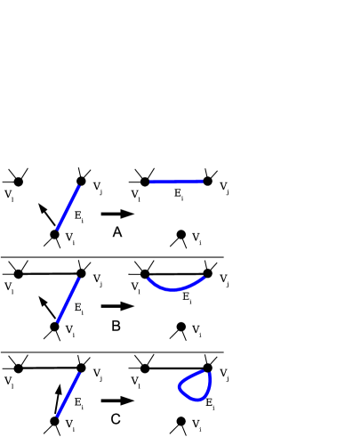
Figure 1: (color online) Illustration of the S-ESP process. The process selects a random edge and rewires it to a node which was preferentially selected. A detailed explanation of preferential selection and the process definition is provided in Section II. The rewiring is unconditional, this means that there is no test of the connectivity state between $V_{l}$ and $V_{j}$. During the rewiring operation the following three cases can occur: In the case A there is no edge between the node $V_{l}$ and the node $V_{j}$, therefore the process does not create a multiple edge or a self loop and it will keep the simple graph property. In the case B there is already an edge between$V_{l}$ and $V_{j}$, and the process adds another edge between the nodes. In the last case C, if $V_{l}=V_{j}$ the process creates a self-loop.

II.1 Simple Edge Selection Process

The Simple Edge Selection Process (S-ESP) is defined by the following steps that are supposed to be repeated in each discrete time unit $t$ (see Fig. 1):

Process 1 (S-ESP)

1. An edge, called $E_{i}$, is selected uniformly at random.

2. An end vertex, called $V_{i}$, of $E_{i}$ is selected uniformly at random. The other end vertex will be called $V_{j}$.

3. A vertex, called $V_{l}$, is selected with a probability proportional to $f(k)$ i.e. with probability $\frac{f(k)}{N\langle f\rangle}$ where $k$ is the degree of $V_{l}$ and $\langle f\rangle$ is the mean value of $f$, $\langle f\rangle\equiv\sum\limits_{s}f(s)P(s)$.

4. The edge $E_{i}$ is rewired from $V_{i}$ to $V_{l}$ i.e. the edge $E_{i}$ between $V_{i}$ and $V_{j})$ is deleted and a new edge between $V_{l}$ and $V_{j}$ is created.

The process keeps the number of nodes and edges in the network constant, and the function $f(k)$ models preferential attachment. Preferential attachment is a concept studied in much detail (see for example barabasi:survey ) that aims at modeling how the agents (processes) in complex networks would choose/search an object on which they want to operate. For example in the complex network of web pages and links, if a web page is updated, the author is often providing links (edges) to other web pages. The links are going to pages (nodes) which are known to the author and these are the pages having already many links pointing to them. In this case, the choice where to link is modeled choosing the function $f(k)$ as $f(k)=k$, i.e. the nodes in step 3 of the S-ESP process are selected with higher probability if they have higher degree.

The S-ESP process captures some aspects, like preferential attachment, of processes in real networks, however, this process generates multiple connections and self-loops, which are rarely observed in real networks. Multiple connections are created, because the edge is rewired irrespective of already existing connections between $V_{j}$ and $V_{l}$. On the other hand, self-loops emerge when vertex $V_{l}$ is the same vertex as $V_{j}$.

To derive the master equation describing the dynamics of the degree distribution for the process above we start with a derivation of the probability term expressing the probability that $V_{i}$ is of degree $k^{\prime}$ and that $V_{l}$ is of degree $k^{\prime\prime\prime}$. The master equation can be constructed parameterizing this term with various values of $k^{\prime}$ and $k^{\prime\prime\prime}$ which express all possible changes in degree of vertices touched by the process step.

Selecting uniformly at random an edge and then selecting uniformly at random an end vertex of this edge is equal to selecting a vertex linearly preferentially Evo i.e. with preference function $f(k)=k$. Therefore, the probability that vertex $V_{i}$ has degree $k^{\prime}$ is given by

$$\text{\bf Prob[}deg(V_{i})=k^{\prime}\text{\bf]}=\frac{k^{\prime}}{N\bar{k}}N(k^{\prime})$$ (1)

Analogically, the probability that $V_{l}$ is of degree $k^{\prime\prime\prime}$ is given by $\frac{f(k^{\prime\prime\prime})}{N\langle f\rangle}N(k^{\prime\prime\prime})$. Since these two selections are independent of each other and since the order of selection is strictly determined, the probability that $V_{i}$ is of degree $k^{\prime}$ and that $V_{l}$ is of degree $k^{\prime\prime\prime}$ is

$$\text{\bf Prob[}deg(V_{i})=k^{\prime}\text{ and }deg(V_{l})=k^{\prime\prime\prime}\text{\bf]}$$

$$=\frac{k^{\prime}}{N\bar{k}}N(k^{\prime})\frac{f(k^{\prime\prime\prime})}{N\langle f\rangle}N(k^{\prime\prime\prime}).$$ (2)

To compute the number $N(k,t+1)$ of vertices having degree $k$ at time $t+1$ one has to consider the number of vertices $N(k,t)$ having degree $k$ already at time $t$ minus the number of all vertices that changed their degree from $k$ to any other value $k^{\prime}\neq k$, plus the number of all vertices that changed their degree from any value $k^{\prime}\neq k$ to $k$. A list of all cases in which the quantity $N(k,t)$ changes its value is provided in Table 1. For example, the first row in Table 1 means that if vertex $V_{i}$ had degree $k+1$ and vertex $V_{l}$ had degree $k-1$ at time $t$, both vertices will have degree $k$ at time $t+1$. Thus, compared to the situation at time $t$ there are two vertices more with degree $k$ at time $t+1$ and this is expressed in the third column of the table.

Degree of $V_{i}$	Degree of $V_{l}$	Change in $N(k)$
$k+1$	$k-1$	$+2$
$k$	$k$	$-2$
$k+1$	$k^{\prime\prime\prime}\neq\{k-1,k\}$	$+1$
$k^{\prime}\neq\{k+1,k\}$	$k-1$	$+1$
$k$	$k^{\prime\prime\prime}\neq\{k-1,k\}$	$-1$
$k^{\prime}\neq\{k+1,k\}$	$k$	$-1$

Table 1: The table provides a list of all cases at time $t$ that lead to a change in the quantity $N(k,t)$ at time $t+1$. The minimal configuration describing changes in $N(k,t)$ for the S-ESP process is shown in Figure 1. The probability that the configuration changes is equal to $\frac{k^{\prime}}{N\bar{k}}N(k^{\prime})\frac{f(k^{\prime\prime\prime})}{N\langle f\rangle}N(k^{\prime\prime\prime})$ as described in the text. The table is used to derive the master equation for the S-ESP (and SG-ESP) process. The master equation is generated using every row in the table exactly once to parameterize the probability configuration term above which describes the probability that the quantity N(k,t) will change. If the degree parameter column contains a set of degree values (as for example in the third row, second column) a summation over this set must be used. The third column contains a multiplier expressing how much the quantity $N(k,t)$ would change.

Now every row of Table 1 is used to generate one term in the master equation as a parametrized version of the basic probability term (II.1). If the degree parameters in the first two columns specify a set of degree values $k$, then a summation over this set must be used. After having calculated the probability of each case multiplied by its effect (the third row of Table 1), we can write down the master equation for the number of vertices with degree $k$ at time $t+1$:

$$N(k,t+1)=N(k,t)$$

$$+2\times\frac{k+1}{N\bar{k}}N(k+1,t)\frac{f(k-1)}{N\langle f\rangle}N(k-1,t)$$

$$-2\times\frac{k}{N\bar{k}}N(k,t)\frac{f(k)}{N\langle f\rangle}N(k,t)$$

$$+1\times\sum\limits_{k^{\prime\prime\prime},k^{\prime\prime\prime}\neq\{k-1,k\}}\frac{k+1}{N\bar{k}}N(k+1,t)\frac{f(k^{\prime\prime\prime})}{N\langle f\rangle}N(k^{\prime\prime\prime},t)$$

$$+...$$ (3)

Writing down all cases and using the fact that $\sum\limits_{s}f(s)N(s)=\langle f\rangle N$ the master equation of the S-ESP process Evo is obtained:

$$N(k,t+1)=N(k,t)-\frac{f(k)}{N\langle f\rangle}N(k,t)$$

$$+\frac{f(k-1)}{N\langle f\rangle}N(k-1,t)-\frac{k}{N\bar{k}}N(k,t)+\frac{k+1}{N\bar{k}}N(k+1,t)$$ (4)

Note that in the above derivation the probability that one selects twice the same vertex, i.e. $V_{l}=V_{i}$, is not taken into account, since this probability is small. Nevertheless, the resulting master equation II.1 is not fully correct. This issue is addressed in evans:bipartite .

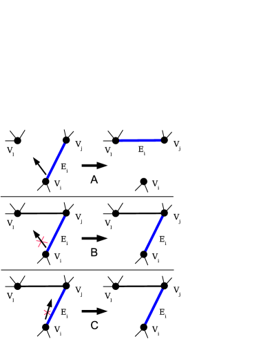
Figure 2: (color online) Illustration of the SG-ESP process. The process selects a random edge and rewires it to a node which was preferentially selected. A detailed explanation of preferential selection and the process definition is provided in Section II. In contrast to S-ESP, according to the SG-ESP process the rewiring occurs only if $V_{l}\neq V_{j}$ and if $V_{l}$ is not directly connected by an edge to $V_{j}$. The process verifies first if there is an edge between $V_{l}$ and $V_{j}$ and if there is no one (case A) the rewiring takes place, otherwise (cases B and C) the process leaves the original edge in place.

II.2 Simple Graph Edge Selection Process

A natural extension of the S-ESP process, which would keep the process within the class of simple graphs is to introduce a connectivity test whether there is an edge between the target nodes, and if one is detected, the rewiring would not take place. The process called Simple Graph Edge Selection Process (SG-ESP) can be defined as follows (see also Fig. 2):

Process 2 (SG-ESP)

The following steps are repeated on a graph $G$ in each discrete time unit $t$.

1. An edge, called $E_{i}$, is selected uniformly at random.

2. An end vertex, called $V_{i}$, of $E_{i}$ is selected uniformly at random. The other end vertex will be called $V_{j}$.

3. A vertex, called $V_{l}$, is selected with a probability proportional to $f(k)$ as in step 3 of the S-ESP process.

   1. Check if $V_{l}$ is an end vertex of $E_{i}$ or if $V_{l}$ is directly connected to $V_{j}$. If so, skip the next step.

4. The edge $E_{i}$ is rewired from $V_{i}$ to $V_{l}$.

The only difference to the S-ESP process is the step 3a. However, to express analytically what this means, one has to know when the condition in step 3a is (not) satisfied. This means to know the probability that a vertex $V_{l}$ is (not) directly connected to an edge $E_{i}$, in other words $V_{l}$ is (not) a direct neighbor of $V_{j}$.

One of the main goals of the present paper is to show that we need to study not only edge distributions but also distributions of higher order objects (wedges) to understand the SG-ESP process in the class of simple graphs. In the next sections we investigate the relations of these distributions and show that they are necessary to analytically express the condition in step 3a of the SG-ESP process.

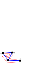
Figure 3: (color online) Wedges are paths of length 2. The graph in this example contains the following 5 wedges: $(V_{3},V_{1},V_{2})$, $(V_{1},V_{2},V_{3})$, $(V_{2},V_{3},V_{1})$, $(V_{1},V_{3},V_{4})$, $(V_{2},V_{3},V_{4})$. The wedge distribution $W(k,k^{\prime},k^{\prime\prime})$ is defined in section II.3. In this example the wedge distribution is $W(1,3,2)=2$, $W(2,3,2)=1$, $W(2,2,3)=2$.

II.3 Higher order distributions

We use the term higher order distribution generally to denote a distribution of more complex objects than nodes. Apart from the degree distribution $P(k)$, the first higher order distribution, which is necessary for further analysis, describes a distribution of edges and is defined as

$$P(k,k^{\prime})=\begin{cases}\frac{1}{2}\frac{L(k,k^{\prime})}{L},&\text{if }k\neq k^{\prime},\\ \frac{L(k,k^{\prime})}{L},&\text{if }k=k^{\prime}.\end{cases}$$ (5)

where $L(k,k^{\prime})$ denotes the number of edges in the network whose end vertices have degree $k$ and $k^{\prime}$, and $L$ denotes the total number of edges in the network. The distribution $P(k,k^{\prime})$ does not describe directly the distribution $\frac{L(k,k^{\prime})}{L}$ but there are two important reasons why the above form of the edge distribution is necessary: a) $P(k,k^{\prime})$ can be interpreted as a probability that a vertex with degree $k$ has a neighbor with the degree $k^{\prime}$, and this form can be directly used for the analysis of the SG-ESP process; b) it is technically simpler to express the relation between $P(k,k^{\prime})$ and $P(k)$ as between $\frac{L(k,k^{\prime})}{L}$ and $P(k)$. Moreover, if needed, $\frac{L(k,k^{\prime})}{L}$ can be easily computed from $P(k,k^{\prime})$.

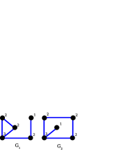
Figure 4: (color online) Two non-isomorphic graphs $G_{1}$ and $G_{2}$ with $N=5,L=5$, where the node degrees are shown. The graphs have the same degree distribution $P(k)=(P(1)=\frac{1}{5},P(2)=\frac{3}{5},P(3)=\frac{1}{5})$ but different edge distributions $P_{G_{1}}(k,k^{\prime})=(P(1,2)=\frac{1}{10},P(1,3)=0,P(2,2)=\frac{1}{5},P(2,3)=\frac{3}{10})$ and $P_{G_{2}}(k,k^{\prime})=(P(1,2)=0,P(1,3)=\frac{1}{10},P(2,2)=\frac{2}{5},P(2,3)=\frac{2}{10})$. The example shows that in general the degree distribution $P(k)$ can not uniquely determine the edge distribution $P(k,k^{\prime})$, but $P(k,k^{\prime})$ determines $P(k)$ according to equation 6.

The edge distribution $P(k,k^{\prime})$ is symmetric, $P(k,k^{\prime})$=$P(k^{\prime},k)$, because in the definition of $L(k,k^{\prime})$ we cannot distinguish which end vertex of the edge has degree $k$ resp. $k^{\prime}$. It was reported clust , that

$$P(k)=\frac{\bar{k}}{k}\sum\limits_{k^{\prime}}P(k,k^{\prime})$$ (6)

and that for uncorrelated networks the edge distribution factorizes, namely $P(k,k^{\prime})=\tilde{P}_{L}(k)\tilde{P}_{L}(k^{\prime})$ where $\tilde{P}_{L}(k)=\frac{kP(k)}{\bar{k}}$.

The next component needed for analysis of the SG-ESP process is a distribution describing probabilities of higher order objects called wedges. A wedge is an object formed by three vertices which are connected together by two edges (a path of length 2, see Fig. 3). Similarly as for edges, we define the wedge distribution as:

$$P(k,k^{\prime},k^{\prime\prime})=\begin{cases}\frac{1}{2}\frac{W(k,k^{\prime},k^{\prime\prime})}{W},&\text{if }k\neq k^{\prime\prime},\\ \frac{W(k,k^{\prime},k^{\prime\prime})}{W},&\text{if }k=k^{\prime\prime}.\end{cases}$$ (7)

where $W(k,k^{\prime},k^{\prime\prime})$ is the number of wedges with the middle node having degree $k^{\prime}$ and one of the end nodes with degree $k$ and the other with the degree $k^{\prime\prime}$. The number of all wedges in the network is denoted with $W$. The wedge distribution is symmetric in both outer arguments, $P(k,k^{\prime},k^{\prime\prime})=P(k^{\prime\prime},k^{\prime},k)$, but in general $P(k,k^{\prime},k^{\prime\prime})\neq P(k^{\prime},k,k^{\prime\prime})$ and $P(k,k^{\prime},k^{\prime\prime})\neq P(k,k^{\prime\prime},k^{\prime})$.

A vertex of degree $k$ is a middle vertex of $\binom{k}{2}=\frac{k^{2}}{2}-\frac{k}{2}$ wedges. Therefore the total number of wedges is fully determined by the degree distribution $P(k)$ and is given by $W=\sqrt{2L^{3}C_{0}}$, where $C_{0}=\frac{\bar{k}}{N}{\left(\frac{\langle k^{2}\rangle-\bar{k}}{\bar{k}^{2}}\right)}^{2}$. It can be shown clust , that $C_{0}$ equals to the clustering coefficient in the case of an uncorrelated network.

To derive the relation between the edge and the wedge distribution we have to consider that $k+k^{\prime}-2$ wedges pass through an edge of degree $(k,k^{\prime})$. Further, considering how many edges a wedge can contribute to and using correct normalization, the following relation for $k,k^{\prime}>1$ is obtained:

$$P(k,k^{\prime})=\sqrt{2LC_{0}}\frac{\sum\limits_{k^{\prime\prime}}P(k,k^{\prime},k^{\prime\prime})+P(k^{\prime\prime},k,k^{\prime})}{k+k^{\prime}-2}$$ (8)

In a different context and differently defined, the distributions of more complex objects have also been studied in wegde ; subgraph ; clustcomp . Another confirmation of the importance of higher order distributions comes from the studies of complex interconnection patterns called network motifs. As the authors of MotifsAsBlocks reported, network motifs observed in the real networks clearly distinguish these networks from artificial randomly generated instances.

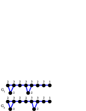
Figure 5: Two non-isomorphic graphs $G_{1}$ and $G_{2}$ with $N=10,L=11$ and $W=15$, where the nodes are labeled with the degrees. The graphs have the same edge distribution $P(k,k^{\prime})=(P(1,2)=\frac{1}{22},P(2,2)=\frac{2}{11},P(2,3)=\frac{7}{22},P(3,3)=\frac{1}{11})$ but different wedge distributions $P_{G_{1}}(k,k^{\prime},k^{\prime\prime})=(...,P(2,2,3)=\frac{1}{10},...)$ and $P_{G_{2}}(k,k^{\prime},k^{\prime\prime})=(...,P(2,2,3)=\frac{2}{15},...)$. In general, an edge distribution can not determine the wedge distribution of a graph, but $P(k,k^{\prime},k^{\prime\prime})$ determines $P(k,k^{\prime})$ according to equation 8.

II.4 Connection probabilities

The wedge distribution introduced in the previous section can be used to express various connectivity probabilities between nodes, edges and wedges. The connection probabilities in turn allow to describe the simple graph constraints.

Assume an arbitrary vertex of degree $k$ and an arbitrary edge of degree $k^{\prime},k^{\prime\prime}$. If $k$ is different from $k^{\prime}$ and $k^{\prime\prime}$, the vertex cannot be part of an edge with degree $k^{\prime},k^{\prime\prime}$. In this case, we can consider a bipartite subgraph, where one partition is represented by $N(k)$ (all vertices of degree $k$) and the other partition is represented by all vertices of the edge set $L(k^{\prime},k^{\prime\prime})$. In this subgraph there are $N(k)L(k^{\prime},k^{\prime\prime})$ possible edges, but only $W(k,k^{\prime},k^{\prime\prime})$ of them are present. Therefore, the probability that an arbitrary vertex of degree $k$ and an arbitrary edge of degree $k^{\prime},k^{\prime\prime}$ are part of the same wedge is $W(k,k^{\prime},k^{\prime\prime})/(N(k)L(k^{\prime},k^{\prime\prime}))$. Similar considerations can also be used for the cases $k=k^{\prime}$ and $k=k^{\prime\prime}$, therefore the probability $P_{k,(k^{\prime},k^{\prime\prime})}$ that a vertex of degree $k$ is directly connected to a vertex of degree $k^{\prime}$ which is a part of an edge of degree $k^{\prime},k^{\prime\prime}$ is given by

$$P_{k,(k^{\prime},k^{\prime\prime})}=\frac{2W\cdot P(k,k^{\prime},k^{\prime\prime})}{(N(k)-\delta_{k,k^{\prime}}-\delta_{k,k^{\prime\prime}})L(k^{\prime},k^{\prime\prime})}$$ (9)

where $\delta_{i,j}$ denotes the Kronecker delta. Analogous reasoning for two distinct vertices leads to the probability that a vertex of degree $k$ is directly connected to vertex of degree $k^{\prime}$. This probability will be denoted as $P_{k,k^{\prime}}$ and is given by

$$P_{k,k^{\prime}}=\frac{2L\cdot P(k,k^{\prime})}{(N(k)-\delta_{k,k^{\prime}})N(k^{\prime})}.$$ (10)

If $k\neq k^{\prime}$ then the edges $L(k,k^{\prime})$ form a bipartite subgraph with the partitions $N(k)$ and $N(k^{\prime})$. Therefore, an arbitrary vertex of degree $k$ participates in $L(k,k^{\prime})/N(k)$ edges of degree $k,k^{\prime}$. In general, the number of edges of degree $k,k^{\prime}$, which an arbitrary vertex of degree $k$ participates in, is denoted as

$$T(k,k^{\prime})=\bar{k}\frac{P(k,k^{\prime})}{P(k)}.$$ (11)

In an analogous way, the number of wedges of degree $k,k^{\prime},k^{\prime\prime}$ which an arbitrary edge of degree $k,k^{\prime}$ participates in is

$$\sqrt{2LC_{0}}\frac{2P(k,k^{\prime},k^{\prime\prime})}{(2-\delta_{k,k^{\prime}})P(k,k^{\prime})}.$$ (12)

This quantity can be also interpreted as the number of edges of degree $k^{\prime},k^{\prime\prime}$ that share the vertex of degree $k^{\prime}$ with another edge of degree $k,k^{\prime}$.

The wedge distribution is useful in many other ways to express the probabilities of connectivity resp. neighborhood relations. For example, the probability that a vertex which is a nearest neighbor of an edge of degree $k,k^{\prime}$ has degree $k^{\prime\prime}$ is given by

$$P(k^{\prime\prime}|k,k^{\prime})=\frac{P(k^{\prime\prime},k,k^{\prime})}{\sum\limits_{k^{\prime\prime}}P(k^{\prime\prime},k,k^{\prime})}.$$

The wedge distribution can also be useful in obtaining more accurate estimations of the local clustering coefficient compared to the situation when only the edge distribution is used (see Natora2007 for further results concerning the wedge distribution).

II.5 Master equation for SG-ESP

To derive the master equation of the SG-ESP process we follow the method introduced at the beginning of this section for the S-ESP process. First, we specify a general probability term describing, for the given configuration of nodes (see Fig. 2), the probability that the configuration change happens i.e. that the edge will be rewired. A list of all possible cases leading to a change in the quantity $N(k,t)$ is the same as for S-ESP (see Table 1).

Three probabilities have to be considered in order to evaluate the overall probability of the configuration change. Firstly, as discussed in the previous sections, $P(k^{\prime},k^{\prime\prime})$ is the probability that vertex $V_{i}$ in Fig. 2 is of degree $k^{\prime}$ and it has a direct neighbor vertex $V_{j}$ of degree $k^{\prime\prime}$. Secondly, $\frac{f(k^{\prime\prime\prime})}{N\langle f(k)\rangle}(N(k^{\prime\prime\prime})-\delta_{k^{\prime\prime\prime},k^{\prime}}-\delta_{k^{\prime\prime\prime},k^{\prime\prime}})$ is the probability that vertex $V_{l}$, which is selected with a probability proportional to $f(k)$, is of degree $k^{\prime\prime\prime}$ and is not a part of the edge $E_{i}$. The last probability to consider is the probability that there is no edge between $V_{l}$ and $V_{j}$. It is equal to $(1-P_{k^{\prime\prime\prime},(k^{\prime\prime},k^{\prime})})$ as discussed above. Putting all together, the probability that the rewiring occurs is given by

$$P(k^{\prime},k^{\prime\prime})\frac{f(k^{\prime\prime\prime})}{N\langle f(k)\rangle}(N(k^{\prime\prime\prime})-\delta_{k^{\prime\prime\prime},k^{\prime}}-\delta_{k^{\prime\prime\prime},k^{\prime\prime}})\times$$

$$(1-P_{k^{\prime\prime\prime},(k^{\prime\prime},k^{\prime})}).$$ (13)

The enumeration of all possible contributions to $N(k,t+1)$ is identical to the S-ESP process, so after summarizing all of them, we obtain the following master equation for the degree distribution. In the equation we suppose that the quantities (as $N(k),P(k^{\prime},k^{\prime\prime})$ and $P_{k,(k^{\prime},k^{\prime\prime})}$) related to some object distribution are functions of discrete time $t$, however in the following text we omit the time variable $t$ to simplify the notation in cases where its presence is clear from the context.

$$N(k,t+1)=N(k)-\sum\limits_{k^{\prime},k^{\prime\prime}}P(k^{\prime},k^{\prime\prime})\frac{f(k)(N(k)-\delta_{k,k^{\prime}}-\delta_{k,k^{\prime\prime}})}{N\langle f\rangle}(1-P_{k,(k^{\prime},k^{\prime\prime})})$$

$$+\sum\limits_{k^{\prime},k^{\prime\prime}}P(k^{\prime},k^{\prime\prime})\frac{f(k-1)(N(k-1)-\delta_{k-1,k^{\prime}}-\delta_{k-1,k^{\prime\prime}})}{N\langle f\rangle}(1-P_{k-1,(k^{\prime},k^{\prime\prime})})$$

$$-\sum\limits_{k^{\prime},k^{\prime\prime\prime}}P(k^{\prime},k)\frac{f(k^{\prime\prime\prime})(N(k^{\prime\prime\prime})-\delta_{k^{\prime\prime\prime},k^{\prime}}-\delta_{k^{\prime\prime\prime},k})}{N\langle f\rangle}(1-P_{k^{\prime\prime\prime},(k^{\prime},k)})$$

$$+\sum\limits_{k^{\prime},k^{\prime\prime\prime}}P(k^{\prime},k+1)\frac{f(k^{\prime\prime\prime})(N(k^{\prime\prime\prime})-\delta_{k^{\prime\prime\prime},k^{\prime}}-\delta_{k^{\prime\prime\prime},k+1})}{N\langle f\rangle}(1-P_{k^{\prime\prime\prime},(k^{\prime},k+1)}).$$ (14)

To see the relation of this equation to the equation for S-ESP (II.1) all terms in the equation above can be expanded in a particular way. For example, after expanding all factors of the last term on the right-hand side of equation (II.5), the term can be written as

$$\frac{k+1}{N\bar{k}}N(k+1)-$$

$$-\sum\limits_{k^{\prime}}\frac{f(k^{\prime})P(k^{\prime},k+1)}{N\langle f\rangle}-\frac{f(k+1)(k+1)}{N^{2}\langle f\rangle\bar{k}}N(k+1)-$$

$$-\sum\limits_{k^{\prime},k^{\prime\prime\prime}}\frac{2W\cdot f(k^{\prime\prime\prime})P(k^{\prime\prime\prime},k^{\prime},k+1)}{N\langle f\rangle L(2-\delta_{k+1,k^{\prime}})}$$ (15)

The other three terms of equation (II.5) can be written in a similar way. This form of equation (II.5) shows that all terms of the S-ESP process are contained in the master equation of the SG-ESP process (the first term in expression (II.5) corresponds to the last term in equation (II.1) etc). The additional terms in (II.5) arise from the simple graph constraint and they show how well and under which conditions the S-ESP process approximates the SG-ESP process. For example, the additional terms become negligible in the limit of $N\gg 1,\frac{W}{N\cdot L}\ll 1$. This is an example of conditions under which simple networks can be treated as non-simple networks, but the equation (II.5) also allows more complex approximations to be investigated.

Graph	$P(k,k^{\prime})$	$P(k)$	$\sum_{k^{\prime}}k^{\prime}P(k^{\prime},2)$
	$\begin{pmatrix}1/2&0\\ 0&1/2\end{pmatrix}$	$\begin{pmatrix}\bar{k}/2&\bar{k}/4\end{pmatrix}$	1
	$\begin{pmatrix}0&1/2\\ 1/2&0\end{pmatrix}$	$\begin{pmatrix}\bar{k}/2&\bar{k}/4\end{pmatrix}$	1/2

Table 2: This example shows that it is not possible to express $\sum\limits_{k^{\prime}}f(k^{\prime})P(k^{\prime},k)$ by $F(f(k),P(k))$, where $F$ denotes an arbitrary function. Consider the two edge distributions in the second column of the table, which describe edges with degree $k,k^{\prime}=1,2$. Further assume that $f(k)=k$. Both edge distribution lead to the same degree distribution (the third column) according to equation 6, but the expression $\sum_{k^{\prime}}f(k^{\prime})P(k^{\prime},2)$ is different.

The counter-examples in Figures 4 and 5 show, that in general it is not possible to obtain $P(k,k^{\prime},k^{\prime\prime})$ from $P(k,k^{\prime})$ or $P(k,k^{\prime})$ from $P(k)$. One can also show by counter-example (see table 2) that $\sum\limits_{k^{\prime}}f(k^{\prime})P(k^{\prime},k)$ cannot be expressed by $F(f(k),P(k))$, where $F$ denotes an arbitrary function. This means that equation II.5 can not be written in a self-consistent way and hence is not solvable in principle. To obtain a closed description we need to consider adding equations for higher order distributions into the system.

Degree of $V_{i}$	Degree of $V_{j}$	Change in $L(k,k^{\prime})$
$k-1$	$k-1$	$+2T(k-1,k^{\prime})$
$k-1$	$\neq\{k,k^{\prime},k-1,k^{\prime}-1\}$	$+T(k-1,k^{\prime})$
$k^{\prime}-1$	$k^{\prime}-1$	$+2T(k^{\prime}-1,k)$
$k-1$	$k^{\prime}-1$	$+T(k-1,k^{\prime})+T(k^{\prime}-1,k)+1$
$k^{\prime}-1$	$\neq\{k,k^{\prime},k-1,k^{\prime}-1\}$	$+T(k^{\prime}-1,k)$
$k$	$k$	$-2T(k,k^{\prime})$
$k$	$\neq\{k,k^{\prime},k-1,k^{\prime}-1\}$	$-T(k,k^{\prime})$
$k^{\prime}$	$k^{\prime}$	$-2T(k^{\prime},k)$
$k$	$k^{\prime}$	$-T(k,k^{\prime})-T(k^{\prime},k)$
$k^{\prime}$	$\neq\{k,k^{\prime},k-1,k^{\prime}-1\}$	$-T(k^{\prime},k)$
$k-1$	$k$	$+T(k-1,k^{\prime})-T(k,k^{\prime})$
$k-1$	$k^{\prime}$	$+T(k-1,k^{\prime})-T(k^{\prime},k)$
$k^{\prime}-1$	$k$	$+T(k^{\prime}-1,k)-T(k,k^{\prime})$
$k^{\prime}-1$	$k^{\prime}$	$+T(k^{\prime}-1,k^{\prime})-T(k^{\prime},k)$

Table 3: Similarly as in Table 1 a list of the cases at time $t$ that will lead to a change in the quantity $L(k,k^{\prime})$ at time $t+1$ is provided. The table gives only the cases where an edge is added and where $k\neq k^{\prime}$. The cases where the edge is deleted are analogical. Cases that follow from permutation are also not listed, for example, the case where $V_{i}$ has degree $k^{\prime}-1$ and $V_{j}$ has degree $k-1$ is not listed, because this case follows directly from the case at line 4 by permutation. When considering all cases for the edge addition (also the permuted ones) a total of 24 is found, analogically we obtain 24 cases for the edge deletion.

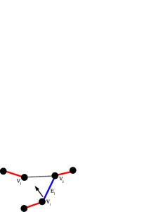
Figure 6: (color online) The randomly selected edge $E_{i}$ touches the edges (red colored) that share a common end-vertex with $E_{i}$. Assuming that $V_{i}$ is of degree $k$ and $V_{j}$ is of degree $k^{\prime}$, the wedge distribution $P(k^{\prime},k,k^{\prime\prime})$ is needed in order to know how many edges of degree $k,k^{\prime\prime}$ share $V_{i}$ as a common end-vertex with $E_{i}$, see expression 12.

To see what are the building blocks of SG-ESP master equations for higher order distributions we consider first the edges. In order to derive a master equation for the edge distribution, all situations at time $t$ which will contribute to $L(k,k^{\prime})$ at time $t+1$ must be enumerated. For example, if $V_{i}$ is of degree $k+1$ we must know how many edges of degree $k+1,k^{\prime}$ participate in $V_{i}$, because all these edges will lose a connection and contribute to $L(k,k^{\prime})$, too. However, vertex $V_{i}$ was not selected independently (like vertex $V_{l}$), but it is an end-vertex of the edge $E_{i}$ (see Fig. 6). Hence, the number of edges of a certain degree which participate in vertex $V_{i}$ is given by expression 12. This expression is proportional to the wedge distribution $P(k,k^{\prime},k^{\prime\prime})$. Therefore, the wedge distribution is needed to derive the master equation for the edge distribution. Moreover, when trying to derive master equations for wedges, the problem persists: In order to know how many wedges of a certain degree share vertex $V_{i}$, which is again part of an edge with prescribed degrees, we need the knowledge of a distribution which is of a higher order than that for wedges.

The analysis above shows that to fully understand the behavior of the SG-ESP process, a whole hierarchy of objects and their distributions must be involved. How far this hierarchy above the wedge distribution is reaching would be very difficult to know, however one conclusion is that the main source of the problems is the edge selection Step 1 of the SG-ESP process and the simple graph constraint. A possibility how to understand more about this complex phenomena and still have a closed description of the process is to introduce more complex vertex selection rules which would approximate the edge selection rule.

III Vertex Based Addition and Deletion of Edges

In this section we describe a class of processes that preserves the simple graph structure and that can be modeled by a single self-consistent equation. This class will be called ”VADE”, which stands for ”Vertex based Addition and Deletion of Edges” and it aims at approximating the edge selection rule of SG-ESP with vertex selection rules. The VADE process is defined as

Process 3 (VADE)

The following steps are repeated on a graph $G$ in each discrete time unit $t$.

1. With probability $q$ do the following:

   1. choose a vertex $V_{i}$ with a probability proportional to $f_{1}(k)$;

   2. choose a vertex $V_{j}$ with a probability proportional to $f_{2}(k)$;

   3. if $V_{i}=V_{j}$ or if $V_{i}$ is directly connected to $V_{j}$, skip the next step;

   4. add an edge between $V_{i}$ and $V_{j}$.

2. With probability $1-q$ do the following:

   1. choose a vertex $V_{l}$ with a probability proportional to $g_{1}(k)$;

   2. Choose a vertex $V_{m}$ with a probability proportional to $g_{2}(k)$;

   3. if $V_{l}=V_{m}$ or if $V_{l}$ is not directly connected to $V_{m}$, skip the next step;

   4. delete the edge between $V_{l}$ and $V_{m}$.

The VADE process is similar to the SG-ESP process in several ways. It contains preferential selection parameters ($f_{1},f_{2},g_{1},g_{2}$), which give the process the flexibility to approximate the edge selection rule of SG-ESP. If the parameter $q$ is chosen appropriately as we discuss at the end of the simulation section, the number of edges is stable in a narrow interval approximating the constant number of edges in the SG-ESP process. The process also preserves the simple graph structure, and the preferential selection parameters can be set to generate a degree distribution which is similar to the one generated by the SG-ESP process (see the simulation study in Section IV).

The reason why the VADE process can be modeled by a self-consistent master equation is that all the selection rules in the VADE process are defined for vertices; in contrast to the SG-ESP process where an edge selection rule is used. Namely, the probability that two vertices are directly connected with each other requires the knowledge of $P(k,k^{\prime})$ (see equation 10), and also only from $P(k,k^{\prime})$ we can derive how many edges of degree $k,k^{\prime}$ participate in a vertex of degree $k$, see expression (11). This is the reason why the dynamics of the VADE process is fully captured in a closed master equation for the edge distribution.

To derive a master equation for this process the two process branches (edge deletion and edge addition) can be analyzed independently and their contributions can be added together. Similarly as for the SG-ESP process, the probability that vertex $V_{i}$ is of degree $k_{i}$, vertex $V_{j}$ is of degree $k_{j}$ and that the conditions mentioned in the step 1c of VADE are not met is given by

$$A(k_{i},k_{j})=\frac{f_{1}(k_{i})f_{2}(k_{j})N(k_{i})\Bigl{(}N(k_{j})-\delta_{k_{i},k_{j}}\Bigr{)}\Bigl{(}1-P_{k_{i},k_{j}}\Bigr{)}}{N^{2}\langle f_{1}\rangle\langle f_{2}\rangle}$$ (16)

The probability that vertex $V_{l}$ is of degree $k_{l}$, vertex $V_{m}$ is of degree $k_{m}$ and that the conditions mentioned in the step 2c of VADE are not met is given by

$$D(k_{l},k_{m})=\frac{g_{1}(k_{i})g_{2}(k_{j})N(k_{m})\Bigl{(}N(k_{m})-\delta_{k_{l},k_{m}}\Bigr{)}P_{k_{l},k_{m}}}{N^{2}\langle g_{1}\rangle\langle g_{2}\rangle}$$ (17)

After the analysis of all situations at time $t$ which will contribute to $L(k,k^{\prime})$ at time $t+1$ (there is a total of 48 such situations, see Table 3), and after considering that $A(k,k^{\prime})$ as well as $D(k,k^{\prime})$ are both symmetric in $k,k^{\prime}$, the master equation for the edge distribution can be written as (again, for notational simplicity the time variable is suppressed on the right hand side)

$$L^{t+1}(k,k^{\prime})=L(k,k^{\prime})+2q\sum\limits_{X}\Biggl{[}A(k-1,X)\left(T(k-1,k^{\prime})+\frac{1}{2}\delta_{k^{\prime}-1,X}\right)+A(X,k^{\prime}-1)\left(T(k^{\prime}-1,k)+\frac{1}{2}\delta_{k-1,X}\right)$$

$$-A(k,X)T(k,k^{\prime})-A(X,k^{\prime})T(k^{\prime}k)\Biggr{]}+2(1-q)\sum\limits_{X}\Biggl{[}D(k+1,X)T(k+1,k^{\prime})+D(X,k^{\prime}+1)T(k^{\prime}+1,k)$$

$$-D(k,X)\left(T(k,k^{\prime})-\frac{1}{2}\delta_{k^{\prime},X}\right)-D(X,k^{\prime})\left(T(k^{\prime},k)-\frac{1}{2}\delta_{X,k}\right)\Biggr{]}.$$ (18)

This equation is valid for $k\neq k^{\prime}$. If $k=k^{\prime}$, the summation term on the right hand side must be multiplied with the factor $1/2$. The four terms proportional to $q$ account for the case when an edge is added, the four terms proportional to $1-q$ account for the case when an edge is deleted. The terms $T(k,k^{\prime})$ account for the edges that change their degree because they participate in one of the involved vertices, whereas the terms $\delta_{k,k^{\prime}}$ account directly for the edge that is added or deleted.

The aim of introducing the VADE process is mainly to show that certain processes can lie in the complexity hierarchy between processes described on the level of the degree distribution and processes having very high description complexity as SG-ESP. VADE also illustrates, which selection rules would bring the most problems thus providing a direction where the next modeling efforts could concentrate. The description of VADE is closed on the edge level and therefore definitively solvable. However, to understand more deeply the relation between SG-ESP and VADE more research would be needed to solve its complex and nonlinear master equation.

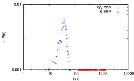
Figure 7: (color online) Simulation experiments for a network with N=1000, L=2000. The x-axis represents degree values and the y-axis the values of $P(k)$, both axes are in logarithmic scale. The processes were simulated over $2.10^{6}$ iterations to the equilibrium state. The figure shows the simulation results for the S-ESP and SG-ESP processes with $f(k)=k$. To obtain the resulting graph a time averaging over 15 instances separated with $10^{4}$ states was computed. The S-ESP process condensates and all edges are rewired to a few nodes (finally to only one node) as self-connections.

IV Simulations

To numerically support the analysis we described in the previous sections, we simulated the S-ESP, SG-ESP and VADE processes. Our experiments focus on small networks and a very long simulation time where a difference between the S-ESP and SG-ESP processes is clearly visible. In all cases we first generated a classical random network with Poisson distribution and average degree 4.0, which was then used as initial condition for all experiments.

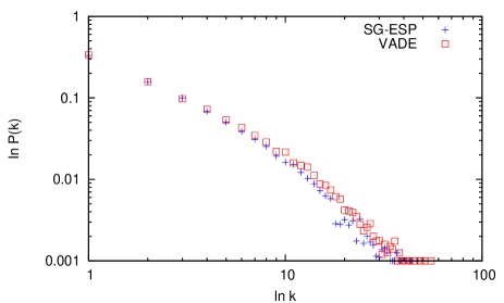
Figure 8: (color online) Simulation experiments illustrating the similarity between the distributions $P(k)$ of VADE and SG-ESP processes. The meaning of the axes is the same as in Figure 7 and the same averaging procedure was used. The parameters for the SG-ESP process are: N=1000, L=2000 and $f(k)=k$ except for $f(0)=5$. The network stabilizes in an equilibrium state with a distribution near to the distribution of a scale-free network. The VADE process was simulated with the parameters: $N=1000,q=0.004,f_{1}(k)=k,f_{1}(0)=1000,f_{2}(k)=k,g_{1}=1,g_{2}=1$.

The experimental results in Figure 7 show that in situations where the effects of simple graph constraints and of finite network size cannot be neglected, S-ESP and SG-ESP behave in a very different way. S-ESP condensates, on the contrary SG-ESP is developing a highly interconnected kernel. The experimental results for the range of parameters in Figure 7 also point to the analysis in mayerdorog , especially in relation to the analysis of the dense network kernel.

Another conclusion from the simulation experiments (see Fig. 8) is that the VADE process can approximate the SG-ESP process very closely due to the flexibility caused by the preferential parameters $f_{1},f_{2},g_{1},g_{2}$. This fact opens a possibility of having new processes which have a closed master equation but which can approximate the SG-ESP process. Figure 8 shows that the VADE process generates a scale free network with very small difference to SG-ESP.

In Figure 9 the number of edges for the VADE process is plotted. The experiments show that if the parameter $q$ of VADE is correctly set the number of edges will stay stable and it will approximate the SG-ESP process. The parameter $q$ can be estimated using the following approximation: the number of edges will stay constant on average if the probability of adding an edge between two vertices with degree $k,k^{\prime}$ is equal to the probability of deleting an edge between two vertices with degree $k,k^{\prime}$. So one has

$$qA(k,k^{\prime})=(1-q)D(k,k^{\prime})$$

$$\Rightarrow q=\frac{1}{1+A(k,k^{\prime})/D(k,k^{\prime})}$$

$$=\frac{1}{1+\frac{f_{1}(k)f_{2}(k^{\prime})(1-P_{k,k^{\prime}})\langle g_{1}\rangle\langle g_{2}\rangle}{g_{1}(k)g_{2}(k^{\prime})P_{k,k^{\prime}}\langle f_{1}\rangle\langle f_{2}\rangle}}$$ (19)

Assuming that $f_{1}(k)=g_{1}(k)$ and $f_{2}(k^{\prime})=g_{2}(k^{\prime})$ this equation will simplify to

$$q=P_{k,k^{\prime}}\approx\frac{2LP(k,k^{\prime})}{N^{2}P(k)P(k^{\prime})}\approx\frac{2L}{N^{2}}.$$

For the last approximation step an uncorrelated network is assumed and both $k$ and $k^{\prime}$ are replaced with $\bar{k}$. For the network parameters in Fig. 8, a value of $q=0.004$ is obtained. This value was used during the experiments and the results are approximating the objective value $L=2000$ very closely (see Figure 9).

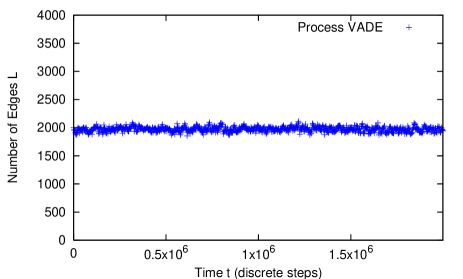
Figure 9: (color online) The figure shows the simulation results for the VADE process with the same parameters as in Figure 8. The x-axis represents the discrete time and the y-axis the number of edges, both axes are in linear scale. The simulation experiments show that the number of edges becomes quickly stable.

V Conclusion

To summarize, the analysis in Section II has shown a method how to describe the process constraining steps that keep a network evolution process in the class of simple graphs. To model these constraints we introduced a new distribution that described wedges - the paths of length 2. The relation between edge distribution (degree-degree correlation) and wedges was also studied to understand the evolution of simple graphs. A combination of such constraints with simple edge selection rules can lead to a very high complexity involving several higher order distributions. How far in the distribution hierarchy one has to go to obtain a closed description of the SG-ESP process is not clear and it would need more research to understand the situation fully. The study of simple graph constraints provides further reasons why it is worthwhile studying (and measuring on real networks) the higher order distributions as for example the wedge distribution.

Up to now, the processes were defined in such a way, that it was possible to formulate a closed master equation for the degree distribution. However these processes either did not respect the simple graph structure or were limited in some other way. When assuming that self-organization is the driving force for the emergence of complex network structures without self-loops and multiple connections, higher order distributions are key, in particular for non-growing simple networks.

The present paper opens several directions for possible research. Further approximations of equation II.5 (or process modes and constraints) can provide deeper insight into the processes on simple graphs or into the parameter ranges where they can be better understood. Another possibility is to study in more detail the intermediate VADE class of processes which are more complex than classical random graphs but simpler than processes containing edge selection rules. These processes can bring more light into the immense complexity of simple graphs through approximation of edge selection rules with more complex set of vertex selection rules.

- (1) M.J. Alava and S. N. Dorogovtsev. Complex networks created by aggregation. Physical Review E, 71(036107), 2005.
- (2) R. Albert and A.-L. Barabási. Statistical mechanics of complex networks. Rev. Modern Phys., 74:47–97, 2002.
- (3) S. N. Dorogovtsev. Clustering of correlated networks. Physical Review E, 69(027104), 2004.
- (4) S. N. Dorogovtsev and J. F. F. Mendes. Evolution of networks. Oxford University Press, 2003.
- (5) S. N. Dorogovtsev, A. M. Povolotsky, and A. N. Samukhin. Organization of complex networks without multiple connections. arXiv.org, (cond-mat/0505193), 2005.
- (6) T. S. Evans and A. D. K. Plato. Exact solution for the time evolution of network rewiring models. Physical Review E, 75(056101), 2007.
- (7) S. Itzkovitz, R. Milo, N. Kashtan, G. Ziv, and U. Alon. Subgraphs in random networks. Physical Review E, 68(026127), 2003.
- (8) J.Ohkubo and T. Horiguchi. Complex networks by non-growing model with preferential rewiring process. Journal of the Physical Society of Japan, 74:1334 –1340, 2005.
- (9) B.J. Kim, A. Trusina, P. Minnhagen, and K. Sneppen. Self organized scale-free networks from merging and regeneration. The European Physical Journal B, 43(3), 2005.
- (10) P. Mahadevan, D. Krioukov, K. Fall, and A. Vahdat. Systematic topology analysis and generation using degree correlations. SIGCOMM, 2006.
- (11) R. Milo, S. Shen-Orr, S. Itzkovitz, N. Kashtan, D. Chklovskii, and U. Alon. Network motifs: Simple building blocks of complex networks. Science, 298(5594):824–827, 2002.
- (12) C. Moore, G. Ghoshal, and M.E.J. Newman. Exact solutions for models of evolving networks with addition and deletion of nodes. Physical Review E, 74(036121), 2006.
- (13) M. Natora. Structure of complex biological networks. Master’s thesis, Department of Computer Science, Institute of Theoretical Computer Science, Department of Physics, Institute of Neuroinformatics, ETH Zurich, 2007.
- (14) M. E. J. Newman. The structure and function of complex networks. SIAM Review, 45(2):167–256, 2003.
- (15) P. Erdős and A. Rényi. On the evolution of random graphs. Magyar Tud. Akad. Mat. Kutató Int. Közl., 5:17 –61, 1960.
- (16) Kwangho Park, Ying-Cheng Lai, and Nong Ye. Self-organized scale-free networks. Physical Review E, 72(026131), 2005.
- (17) N. Sarshar and V. Roychowdhury. Scale-free and stable structures in complex ad hoc networks. Physical Review E, 69(026101), 2004.
- (18) M. Angeles Serrano and Marian Boguna. Clustering in complex networks. i. general formalism. arxiv.org, (cond-mat/0608336), 2006.