90 GHz and 150 GHz observations of the Orion M42 region.
A sub-millimeter to radio analysis.

Abstract

We have used the new 90 GHz MUSTANG camera on the Robert C. Byrd Green Bank Telescope (GBT) to map the bright Huygens region of the star-forming region M42 with a resolution of 9^′′ and a sensitivity of 2.8 mJy beam^-1. Ninety GHz is an interesting transition frequency, as MUSTANG detects both the free-free emission characteristic of the H II region created by the Trapezium stars, normally seen at lower frequencies, and thermal dust emission from the background OMC1 molecular cloud, normally mapped at higher frequencies. We also present similar data from the 150 GHz GISMO camera taken on the IRAM 30 m telescope. This map has 15^′′ resolution. By combining the MUSTANG data with 1.4, 8, and 21 GHz radio data from the VLA and GBT, we derive a new estimate of the emission measure (EM) averaged electron temperature of $T_{e}\,=\,11376\pm 1050$ K by an original method relating free-free emission intensities at optically thin and optically thick frequencies. Combining Infrared Space Observatory-longwavelength spectrometer (ISO-LWS) data with our data, we derive a new estimate of the dust temperature and spectral emissivity index within the 80^′′ ISO-LWS beam toward Orion KL/BN, $T_{d}\,=\,42\pm 3\,K$ and $\beta_{d}\,=\,1.3\pm 0.1$. We show that both $T_{d}$ and $\beta_{d}$ decrease when going from the H II region and excited OMC1 interface to the denser UV shielded part of OMC1 (Orion KL/BN, Orion S). With a model consisting of only free-free and thermal dust emission we are able to fit data taken at frequencies from 1.5 GHz to 854 GHz (350 $\mu$m).

1. INTRODUCTION

The Orion Nebula (M42), located 437$\pm$19 pc from the Sun (Hirota et al., 2007), is one of the closest regions of active high mass star formation. This H II region, which lies in front of the OMC1 molecular cloud, is excited by a group of OB stars known as the Trapezium. The OMC1 molecular cloud is part of a bigger complex that extends over 30^∘ of the sky. It is an ideal site for the study of star formation and the physics of the interstellar medium (ISM). The M42 area has been extensively mapped across the electromagnetic spectrum (see O’Dell, 2001, for a review). This area contains hot young stars located in the Trapezium, pre-stellar cores, and regions of dense molecular gas. With multi-wavelength observations the properties of these different regions and how they interact can be understood.

In this paper we report on some of the first scientific observations at 90 GHz using the 100 m diameter Robert C. Byrd Green Bank Telescope (GBT). A 9^′′ resolution $5^{\prime}\times 9^{\prime}$ continuum map in the bright Huygens region of M42 was made using the new MUSTANG focal plane array described in Section 2. To confirm the reliability of the MUSTANG images, two independent data analysis pipelines were used. These are described in Sections 4.1 and 4.2.

At 90 GHz the Huygens region is bright, not simply with free-free radiation from the ionized gas but also, in remarkably equal measure, with thermal dust radiation from the molecular cloud. However, the two emission components have quite different spatial structure. We were able to separate them using data at higher and lower frequencies between 1.5 GHz and 854 GHz. These data are presented in Section 5. We describe the morphology of OMC1-M42 as seen over this frequency range in Section 6. In Section 7, we derive an estimate of the electron temperature and in Section 8, we study the dust emission. The results are summarized in Section 9.

2. THE MUSTANG CAMERA

MUSTANG, the MUltiplexed Squid TES Array at Ninety GHz (Dicker et al., 2008) is a continuum camera built as a user instrument for the GBT. At the heart of the instrument is an $8\times 8$ focal plane array of Transition Edge Sensor (TES) bolometers built at NASA/GSFC. Two high density polyethylene lenses reimage the Gregorian focus of the GBT onto the detectors with an effective focal length of 162 m so that each detector is spaced on the sky by $4.2^{\prime\prime}$, approximately $0.5f\lambda$. A $4.2^{\prime\prime}$ spacing fully samples the sky in a single pointing of the GBT, decreasing the need for fast ($>$0.1 Hz) chopping or scanning in order to reduce $1/f$ noise. Slow movements of the telescope ($\sim 1^{\prime}$ per second) produce many redundant measurements of each point in the field of view which can be used to remove much of the noise on timescales from 0.07 s to 0.5 s (the time it takes a source to move between pixels and across the array). The scan pattern constrains $1/f$ noise on time scales longer than $\sim$5 s (the time between observations of the same part of the sky). Lower scanning speeds are a great advantage as large accelerations can excite oscillations in the GBT’s structure making accurate pointing problematic.

MUSTANG has an 81 GHz to 99 GHz bandpass. Its optical system provides a uniform illumination of the primary mirror of the GBT out to a radius of 45 m and zero elsewhere. A best fit Gaussian to the measured beam shape has a FWHM of 9^′′, close to the value predicted by optical models of the instrument. Below 10 dB the measured beam is significantly higher than that expected from a perfect telescope. This is due to power being scattered from small errors in the shape of the GBT’s primary mirror that occur on length scales of 1–10 m. During the observations presented in this paper, the surface had a 390 $\mu\rm{m}$ RMS, consistent with our measured beam efficiency of 10%. Since these observations were made there have been significant improvements to the GBT’s surface and our measured beam efficiency is currently (in March 2009) around 20%.

The output from each detector is obtained at a software selectable rate which for these observations was 1 kHz. The data values are relative to an arbitrary but stable zero point and are in arbitrary units of “counts”. The conversion of counts to flux units depends on each detector’s gain which varies depending on several factors including the bias voltage and the location of the TES on its transition. The gain of the detectors can be measured using a small black body, “CAL”, located at the Lyot stop so it uniformly illuminates all the detectors. Tests have shown detector gains to be stable to better than a few percent over many hours.

3. OBSERVATIONS

The MUSTANG map is the result of 5.6 hours of integration time yielding a final map RMS of 2.8 mJy beam^-1. Observations were conducted over 4 sessions in January and February 2008. Each observing session was begun by mapping the primary calibrators Mars or Saturn. In this paper we use the Ulich (1981) measurement for the 90 GHz brightness temperature of Saturn, $T_{B}=149.3$ K. Every 30 minutes focus and pointing corrections were measured and applied by collecting small maps of a bright source at a range of focus settings. In cases where these data indicated that the pointing correction was significantly less than MUSTANG’s instantaneous field of view, corrections were applied in the data analysis offline. The bright quasar 0530+135 was used for this purpose as it is unresolved and is located only several degrees away from M42. The gains of the detectors were measured by taking a 30 second scan while pulsing CAL at 0.5 Hz. Another 30 second scan on a blank piece of sky was taken to aid with estimations of the weights used when co-adding data from different detectors.

When scanned across the sky a fully-sampled imaging detector array such as MUSTANG produces many redundant measurements of a given Nyquist sky pixel. In addition to the sky signal, systematic signals (e.g., atmospheric emission and gain drifts) are present. For a well-designed system these will change slowly compared to the sky signal and have a different characteristic signature in the detector time stream. This is facilitated by an appropriate sky modulation (scan) pattern. Furthermore, most of the dominant systematic signals — in particular atmospheric emission and thermal drifts in the receiver — are common-mode between detectors. Provided that the sky map is highly oversampled on most spatial scales it is, in principle, straightforward to form high-quality astronomical images.

M42 was mapped primarily with tiled $5^{\prime}\times 5^{\prime}$ “box” scans which take 5 minutes each. The telescope is scanned diagonally across the rectangular area being mapped at a constant speed, turning around at the edges with a gentle acceleration so as to minimize resonances in the GBT’s structure (Figure 1). The scan speed is chosen so that all astronomical objects with spatial scales smaller than a few arcminutes pass through the beam in under 5 seconds, a timescale faster than changes in the atmosphere or instrumental response. This scan pattern generates uniform coverage with a high degree of cross linking on many different timescales enabling low frequency instrumental and atmospheric signals to be removed. The $5^{\prime}\times 9^{\prime}$ selected region of M42 was mapped in sets of 6 box scans on subdivided north and south fields. To provide additional cross linking, the central pointing of each scan was offset from the previous one by a non-integral multiple of the spacing between crossings.

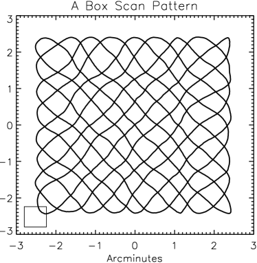
Figure 1.— The GBT boresight trajectory on the sky during the “box” scan pattern used in our observations. The square in the bottom left represents MUSTANG’s 33.6^′′ square field of view.

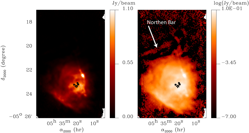
Figure 2.— The M42 MUSTANG map reduced with Obit (Section 4.2). The large dynamic range, over a factor of 1000, can be seen by comparing the linear scale (left) and the logarithmic scale (right). Shown on each map are the Trapezium stars with the bigger one being $\Theta^{1}$ C Ori, the main ionization source.

4. MUSTANG DATA REDUCTION

MUSTANG’s data were reduced using two independent pipelines. The first, written in IDL, implements a least-squares map-making approach explicitly solving for instrumental parameters and sky pixel values. The second, known as Obit (Cotton, 2008), is an iterative algorithm that uses a single-dish implementation of CLEAN. The following subsections describe each approach. Several general properties of the MUSTANG data are worth noting:

1. The largest signal component is due to atmospheric emission. Due to the large size of the GBT and the small divergence of the beams, each detector samples the same volume of atmosphere. Once the detectors are properly calibrated this signal is almost completely common mode.

2. There is also a strong component due to MUSTANG’s pulse tube cooler causing temperature fluctuations in the optical path. This signal is nearly perfectly sinusoidal and its frequency is very stable at $1.4117\pm 0.005\,{\rm Hz}$. The best way to remove this signal was found to be by fitting a sine wave with a slowly varying amplitude to the low pass filtered time streams.

3. There are significant ($0.1-0.2$ second) absolute timing offsets in the MUSTANG data. At our typical slew speeds of $1^{\prime}$ per second this corresponds to pointing offsets in the scan direction comparable to the MUSTANG beam. A 1 pulse-per-second (1PPS) signal is available in the GBT receiver room which demarks UTC second boundaries. This is sampled synchronously with the detectors and used to correct the instrument’s timestamps offline.

Since most of the systematic effects are common mode and a naive common mode subtraction will remove any sky structures larger than the instantaneous field of view, we wanted to carefully test the efficiency of our imaging algorithms at retrieving the large scale emission. Consequently we analyzed the data with two independent approaches and compared the resulting maps, as described in the following sections.

4.1. Least Squares Map Making

The map-making problem can be framed as a large linear least squares problem. As an example consider that we have $N_{det}$ detectors, each yielding $N_{int}$ integrations for a total of $N_{tot}=N_{det}\times N_{int}$ data points. The time stream data can be represented by a single data vector $\Delta$ with $N_{tot}$ components. The observation covers a map comprising $N_{pix}\ll N_{tot}$ sky pixels. Furthermore we allow $N_{par}\ll N_{tot}$ parameters to describe instrumental systematics — for instance, a slowly varying common mode due to sky emission and a set of fixed detector gains. The sky plus instrument model parameters are represented by a vector, $\delta$, with $N_{pix}+N_{par}$ parameters. If the instrument model is linear, or linearizable, the data are related to the model parameters by a $N_{tot}\times(N_{pix}+N_{par})$ matrix $H$ by the equation

$$\Delta=H\delta$$ (1)

As long as $N_{tot}>N_{pix}+N_{par}$, and $H$ is non-singular, a solution of the form

$$\delta=(HWH)^{-1}\,HW\,\Delta.$$ (2)

exists where we have introduced a weight matrix, $W$, describing the noise and correlations in the time stream data. An advantage of this approach is that it is possible to explicitly determine the uncertainties in the resulting instrument and sky model parameters as well as their correlations. This approach has been widely used for imaging the Microwave Background and in other deep extragalactic experiments (e.g., Tegmark, 1997; Patanchon et al., 2008). Two difficulties are present. First, the matrix $HWH$ is of size $(N_{pix}+N_{par})^{2}$, which can be unwieldy if treated with brute force. Second, if we desire to solve for detector gains, the problem is no longer linear in the model parameters, but rather is bilinear due to ${\rm gain}\times{\rm sky\,pixel}$ terms.

Fixsen et al. (2000) have implemented an iterative solution to Eq. 2 which, for typical data sets, can be executed quickly on modern desktop computers. We have integrated their least squares imaging routines into an IDL data analysis pipeline initially developed by the project team for quick-look and exploratory data reduction. Several models are provided by the Fixsen et al. (2000) code. We have explored variants of a model of the form

$$\Delta=G(S+A)+F,$$ (3)

where $G$ is a set of detector gains, $S$ is the sky (astronomy) model, $A$ is a common mode optical loading term, and $F$ is a per-detector additive offset. Care must be taken that the number of model parameters do not become excessive, which can be done by a combination of selecting a long solution interval for the variable terms, and by fixing or eliminating degenerate terms. For the MUSTANG data presented in this paper a comprehensive noise characterization was not necessary. The weight matrix $W$ was assumed to be diagonal with per-detector variances determined every half hour from the time stream model residuals. Imaging fainter extended sources will benefit from a more accurate treatment.

The final least squares map was produced by imaging roughly half-hour long sets of scans and coadding the resulting images, properly accounting for the pixel weight distributions. The $G\times A$ models have an exact degeneracy which corresponds to an arbitrarily oriented two-dimensional linear ramp in pixel intensities across the map. This was eliminated by fitting a plane to two orthogonal, approximately emission-free lines of pixels in each half-hour map and subtracting it before coaddition.

4.2. The iterative CLEAN algorithm — Obit

The basic approach used in the Obit reduction of MUSTANG data is to iteratively estimate the background signal and the astronomical signal (the “sky model”). At the start of each iteration loop, the current sky model is subtracted from the time stream data and the background signals (atmosphere, detector, etc.) are estimated by low-pass filtering the residual. These backgrounds are then removed from the original time streams, an observed sky image is produced, and the true sky estimated using CLEAN. The sky model and the backgrounds are iteratively refined by reducing the timescale of the low-pass filter used in the background estimation as the iteration progresses.

Time stream data are imaged by multiplying each datum with a griding kernel producing a continuous function which is then sampled onto a regular celestial grid. Two grids are accumulated. The first grid, the image, contains the data samples multiplied by a data weight and the griding function. The second grid contains the data weights multiplied by the griding function. When all data are accumulated, the image is normalized by dividing by the second grid on a pixel-by-pixel basis. The griding kernel was chosen to minimize the broadening of the instrumental response and is an exponential times a sinc function.

There are two types of operations used by Obit, those done independently on each 5 minute scan and those which are coupled to all data through the sky model. The independent processing steps are the following.

1. Reading archive data. The kHz sampled data are read and averaged to a 20 Hz rate. Then the 1.4117 Hz signal from the pulse tube refrigerator is estimated and removed by fitting a sine wave with a common phase and a detector-dependent amplitude.

2. Gain calibration. Detector gains are determined from the half hourly CAL scans. These gains are applied to all subsequent data until the next calibration scan. Calibration to Jansky is achieved from observations of planets.

3. Weight calibration. Statistical weights are determined for each detector during blank sky observations by the RMS residuals following the fitting and removal of a low order polynomial from the data. Dead and badly behaving detectors are given zero weight.

4. Common atmosphere and detector offsets. A single detector offset per scan and a time variable common “atmospheric” term is estimated by low pass filtering the median of all working detectors in each time sample.

When these operations are complete, multiple scans over multiple days can be jointly imaged and non-astronomical backgrounds removed. The imaging/background removal cycle consists of the following.

1. Imaging. The current estimates of the backgrounds are removed and all data are accumulated onto a common grid and normalized to form the “Raw” image.

2. Deconvolution. CLEAN is used to generate a sky model consisting of delta functions. Fixed or interactive specification of the CLEAN windows is used to guide the process.

3. Subtracting the model. The CLEAN delta functions are convolved with a Gaussian approximation to the telescope beam shape. The value corresponding to each data sample is interpolated from this CLEAN image and subtracted from the time stream data. This results in a residual time stream in which the current estimate of the astronomical signal has been removed.

4. Estimation of the background. An estimation of the background signal is made by low pass filtering of the residual time stream data. This filtering alternates between estimating individual detector offsets and a common mode offset estimated with shortest time scales one third of that used for the detector offsets.

After the cycles have converged, the final CLEAN image is used for subsequent analysis.

4.3. Comparison of Results

The map produced by the Obit pipeline is shown in Figure 2. On a linear scale the Obit maps are very similar to those produced by least squares. The peak height of Orion KL, the brightest feature in the maps was within 5% of each other and neither data pipeline produced significant negative flux. For bright features, all extended structure on angular scales up to 2^′ was recovered. The most prominent discrepancies between the maps were faint extended structures in the north of the maps which have higher signal-to-noise in the Obit maps. Given the similarity of the maps produced by independent analysis we believe all of the features above the stated noise level to be real.

5. ORION AT OTHER FREQUENCIES

Table 1A summary of the different frequency maps used in this paper.

Map	$\lambda$	$\nu$	FWHM	largest Angular	Relative	RMS	RMS
	(mm)	(GHz)	(′′)	Scale (′)	uncertainty	(MJy sr-1)	(mJy beam-1)
SHARC-II 350	0.35	854	9	$>2$	30%	509	1100
SCUBA 450	0.45	664	8a	1.1	30%	106	300
SCUBA 850	0.85	352	15a	1.1	15%	5.8	40
GISMO	2.0	150	15	$>2$	20%	17	100
MUSTANG	3.3	90	9	2	15%	1.3	2.8
$K$ band	14	21.5	33.5	6	15%	6	180
$X$ band	35	8.4	8.4	2	15%	3.7	7
$L$ band	200	1.5	7	14	15%	2.8	3.6

^a The SCUBA beam shapes consist of a core Gaussian with a FWHM given in this table and a broad component with a relative peak intensity of 5% of the core and a FWHM of 30^′′ (Johnstone et al., 2006).

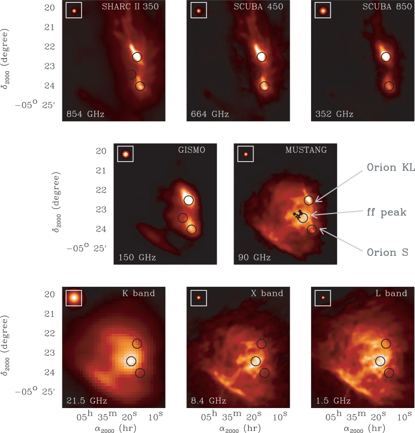
Figure 3.— Maps of M42. All datasets are displayed with their nominal resolution. The inset boxes in each map display Gaussian approximations to the point-spread-functions. The 30^′′ circles on each map delineate areas used to compute average spectra at Orion KL, Orion S and the free-free emission peak locations (shown in Figure 5). Shown on the MUSTANG map are the Trapezium stars with the bigger one being $\Theta^{1}$ C Ori, the main ionization source.

Figure 4.— A false color map of the Orion bar. The SCUBA 850 $\mu$m image is shown in blue, the IRAC $8\,\mu$m map is shown in green, and red is the MUSTANG data. The profiles displayed correspond to the cut shown on the map, starting from the upper right and moving away from the Trapezium stars which are located toward the northwest of this map.

Figure 5.— Average spectra over the areas delineated by the 30^′′ diameter circles on Figure 3. The dot-dashed line is the free-free emission component, the dashed line is the thermal dust emission component and solid line is the total. For comparison, the dotted line shows the free-free emission without taking account of the opacity. This fitted function is described in the Appendix.

To interpret the MUSTANG data we made comparisons to maps at other frequencies. These included a 854 GHz (350 $\mu$m) SHARC-II map and the 664 GHz (450 $\mu$m) and 352 GHz (850 $\mu$m) maps from SCUBA (Johnstone & Bally, 1999). We obtained new 150 GHz maps using data from GISMO (Staguhn et al., 2008) and radio frequency data at 21.5 GHz, 8.4 GHz, and 1.5 GHz ($K$ band, $X$ band, and $L$ band) from the GBT and the VLA. A summary of the angular resolution, RMS, and calibration uncertainties of each of these maps is given in Table 1. In order to compare them, all the maps were converted to MJy sr^-1 by dividing by the solid angles of their respective beams.

5.1. The 1.5 GHz map

The image of M42 at 1.5 GHz (20 cm) was derived from archival VLA data taken with the VLA in “B”, “C”, and “D” configurations. This combination of configurations gives sensitivity to angular scales between 14^′ and 4^′′. Initial calibration of the data were carried out in AIPS using standard VLA flux density calibrators (3C48, 3C138, and 3C2860) and B0500$+$019 as an astrometric calibrator.

After the individual observations were calibrated, they were concatenated and processed in Obit. Automated flagging of RFI was followed by an imaging using the “SDI” technique (Steer et al., 1984). This technique uses a standard visibility-based CLEAN to the point that the fine scale structure has been removed from the residual and only a large, flat plateau is left. In subsequent iterations, a CLEAN component is added at the location of each residual pixel above a given limit. This suppresses instabilities inherent with CLEAN that can produce artifacts for very extended sources. Twenty one facets were used to cover the full field of view as well as outlying sources. Twenty million CLEAN components with a total flux density of 324 Jy were used in the deconvolution. A Briggs Robust weighting parameter of -0.5 gave an approximately 7^′′ FWHM beam and the restoration used a 7^′′ FWHM Gaussian beam.

5.2. The 8.4 GHz Map

The 8.4 GHz image was made by combining continuum observations from the GBT and the VLA. Data from the GBT was taken in an “On-The-Fly” raster mode and contains information on angular scales from the size of the map down to the limit of the GBT’s resolution at 8.4 GHz (1.46^′). The VLA data, taken with the array in “D” configuration, are a series of tiled $3^{\prime}\times 3^{\prime}$ pointings and contain information on spatial scales from those of the shortest to the longest baselines (2^′ to 8.4^′′). These data sets were combined using AIPS++ and CASA to produce a single map with a very high dynamic range and sensitivity to all structures down to a FWHM resolution limit of 8.4^′′.

5.3. The 21.5 GHz Map

A 21.5 GHz continuum map of M42 was obtained from archival GBT data and reduced in IDL. The data were collected using the GBT’s Digital Continuum Receiver (DCR), a general-purpose continuum back end. An internal noise calibration source with a known noise temperature was pulsed once within each integration and the data were calibrated to antenna temperature using this noise source. Data were collected with simple, cross-linked raster scans 12^′ long in Right Ascension and Declination. A DC offset and a gradient were removed from each scan, and the resulting data gridded onto the sky. The resulting map contains information on angular scales from 6^′ to 33.5^′′, the resolution of the GBT at 21.5 GHz.

5.4. The 150 GHz GISMO Map

GISMO is another TES bolometer camera built to operate at 150 GHz on the 30 m IRAM telescope (Staguhn et al., 2008). The data presented in this paper were obtained during the first run with the instrument in November 2007. A “data cleaning” routine was used to remove spikes in the data and to identify bad pixels. Since the weather was exceptionally good ($\tau_{225}=0.07$) a high-pass filter with a low frequency cutoff at 0.2 Hz removed most of the atmospheric noise. After this step a visual inspection of the data of each individual pixel was carried out and pixels with spikes or steps that were not already identified by software were flagged as bad. Per-pixel gains and offsets were then calculated by fitting a linear function to the correlation between the time series of data for each single pixel and the time series of median values for each frame. Pointing and flux calibrations were obtained by observations of quasars and planets. The total integration time for the part of the map shown in this paper was about 4 minutes. A combination of fast scanning and GISMO’s $2^{\prime}\times 4^{\prime}$ instantaneous field of view ensured that all extended structure up to (and probably beyond) an angular size of 2^′ was recovered.

5.5. The SCUBA Maps

We used maps of the Orion ridge originally observed by Johnstone & Bally (1999). The data were taken of a 50^′ long region over four nights with the SCUBA instrument on JCMT. The observations consist of a number of 10^′ by 10^′ maps made with chop throws of 20^′′, 30^′′, and 65^′′. By combining maps made with these different chop throws and different chop directions all extended structures with angular sizes up to the largest chop size (65^′′) were recovered.

5.6. The SHARC-II Map

We used the SHARC-II camera (Dowell et al., 2003) on the Caltech Submillimeter Observatory to obtain a 350$\mu m$ (854 GHz) map. The absolute uncertainty for this measurement is $\sim\,30\%$ and the beam size is 9^′′. SHARC-II’s field of view is $2.59^{\prime}\times 0.97^{\prime}$ so it can be expected that all extended structure with angular scales less than 2^′ is included in our map.

6. THE MORPHOLOGY OF M42-OMC1

Figure 3 displays maps of the eight datasets we used. Each dataset is presented at its nominal resolution. At 21.5, 8.4 and 1.5 GHz ($K$ band, $X$ band, $L$ band), the observed intensity is entirely dominated by free-free emission from the ionized gas around the OB stars of the Trapezium, since there is no evidence for significant synchrotron emission in M42 as noted by Subrahmanyan et al. (2001). At higher frequencies, the SHARC-II (854 GHz) and SCUBA (664 and 352 GHz) maps are dominated by thermal dust emission of the OMC1 molecular cloud lying behind the ionized gas. The two brightest features seen with the thermal dust emission are Orion KL/BN and Orion S. At 90 GHz, free-free and thermal dust emission have about the same intensity in this region, and so both the ionized gas and the OMC1 molecular cloud are seen in the MUSTANG map. As the spectral shape of the dust emission is quite steep compared to free-free emission, this equipartition vanishes rapidly when looking at a different frequency. Thus, the spatial structure in the GISMO map is dominated by the OMC1 features with only a relatively low contribution from ionized gas.

To the southeast of the Trapezium stars is the well known “Orion bar” associated with the edge-on boundary between the H II region and the molecular cloud. A close up of the bar is shown in Figure 4. The clear shift in the position of the bar at different frequencies is what one would expect at the ionization front. Moving away from the exciting stars, one sees first the ionization front emitting strongly at 90 GHz due to high emission measure (EM), next comes the mid-infrared emission bands of polycyclic aromatic hydrocarbons from the photodissociation region seen with IRAC 8 $\mu$m (Megeath et al., 2005) and finally, the molecular material which is bright at the SCUBA 352 GHz (850 $\mu m$) frequency due to the high column density of dust. Note that another much fainter bar can be seen in the MUSTANG map to the north-east of the Trapezium at $\alpha_{2000}\sim 5^{h}\,35^{\prime}\,23^{\prime\prime}$ and $\delta_{2000}\sim-5^{\circ}\,20^{\prime}\,20^{\prime\prime}$ (Figure 2). This bar has already been detected at radio frequencies (Yusef-Zadeh, 1990) and with molecular tracers (Fuente et al., 1996; Rodriguez-Franco et al., 1998).

The spectra in Figure 5 are those observed at the free-free emission peak, and at the Orion KL/BN and Orion S locations. These are the averaged spectra over the areas delineated by circles on Figure 3. Before averaging each map was brought to the spatial resolution of the 21.5 GHz map (33.5^′′) by convolving it with a Gaussian of appropriate FWHM. Spectra were fitted using the function described in the Appendix. As noted previously, at the MUSTANG frequency (90 GHz), the emission toward Orion KL/BN has almost equal contributions from thermal dust and free-free emission. However, toward the free-free emission peak, free-free emission dominates the MUSTANG intensity and even the GISMO one at 150 GHz.

Table 2A comparison between our EM values and those of Baldwin et al. (1991).

location relative	Baldwin et al.	this paper
to $\theta^{1}\,Ori\,C$	(${\rm pc\,cm}^{-6}$)	(${\rm pc\,cm}^{-6}$)
30′′ west	$8.8\times 10^{6}$	$8.2\pm 1.1\times 10^{6}$
50′′ west	$4.3\times 10^{6}$	$3.8\pm 0.5\times 10^{6}$
100′′ west	$8.8\times 10^{5}$	$5.3\pm 0.7\times 10^{5}$

Toward the free-free emission peak, we obtained an emission measure (EM) value of $7.6\pm 0.8\times 10^{6}\,{\rm pc\,cm}^{-6}$ in a 33.5^′′ FWHM beam. This value can be compared with a value of $2.7\times 10^{6}\,{\rm pc\,cm}^{-6}$ in a 90^′′ FWHM beam at 10.55 GHz by Subrahmanyan et al. (2001). Taking into account the beam dilution from 33.5^′′ to 90^′′, we obtained a value of $5.1\pm 0.5\times 10^{6}\,{\rm pc\,cm}^{-6}$, a factor $\sim 1.9$ above the Subrahmanyan et al. (2001) value. This discrepancy could, in part, come from the fact that they used a differencing receiver which could potentially miss flux on spatial scales similar to the separation of the feeds. We can also compare our EM estimate with those of Baldwin et al. (1991) that were deduced from H11-3 measurements. We derived an EM map (Figure 6) with 8.4^′′ resolution using only the 8.4 GHz ($X$ band) and 1.5 GHz ($L$ band) data which can be directly compared with the East-West cut toward the West of $\theta^{1}$ Ori C given by Baldwin et al. (1991). As can be seen in Table 2 both the absolute value and the spatial variation of our radio estimate of EM are in good agreement with their optical one.

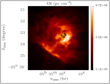
Figure 6.— A map of the emission measure derived from the 8.4 GHz and 1.5 GHz data at 8.4^′′ resolution. The stars show the location of the Trapezium stars.

We found that no anomalous emission component is needed to reproduce data at all frequencies and angular scales ($<1.1^{\prime}$) considered in this paper. A number of detections of such emission have been made in other parts of the sky, for example Kogut et al. (1996) found an excess between 30 GHz and 90 GHz at high latitudes in COBE data. This excess is correlated with DIRBE far-infrared data and has since been interpreted as arising from spinning dust (e.g., Lazarian & Finkbeiner, 2003). Excess emission on large spatial scales has also been detected at frequencies of 15 GHz and 30 GHz by Leitch et al. (1997) and at 33 GHz and 43 GHz by de Oliveira-Costa et al. (1997). Anomalous emission was also observed toward individual objects such as H II regions (e.g., Dickinson et al., 2006, 2009), cold dense clouds (e.g., Casassus et al., 2006) and planetary nebula (e.g., Casassus et al., 2007). Emission from spinning dust is thought to peak between 10 GHz and 50 GHz so a small component could be missed in our analysis. (Lazarian & Finkbeiner, 2003). In order to check for the presence of anomalous emission, new data at $Ka$ band (27 GHz–42 GHz) have been obtained and analysis is currently underway.

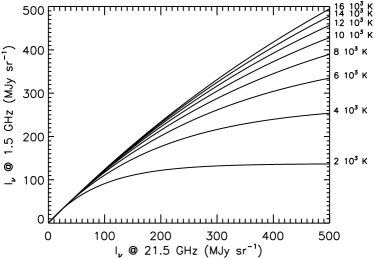
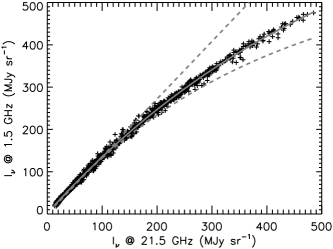
Figure 7.— Modeled (top panel) and observed (bottom panel) relationships between 1.5 GHz and 21.5 GHz free-free emission intensities. On the bottom panel, in gray, is the relationship for the fitted electron temperature of $T_{e}\,=\,11376$  K. For comparison, the curved dashed line is the expected relationship for $T_{e}\,=\,7865$ K (Subrahmanyan, 1992) and the straight dashed line is the expected relationship without opacity (i.e. $T_{e}\,=\,\infty$).

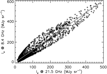
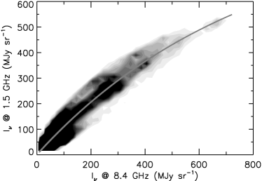
Figure 8.— Relationship between 21.5 GHz and 8.4 GHz (top panel) and 8.4 GHz and 1.5 GHz (bottom panel) free-free emission intensities. For the bottom panel, we show the histogram of points density in gray-scale. Gray lines are the fitted relationship (see Section 7).

7. $T_{e}$ determination from the free-free intensity relationship

Assuming that free-free emission is optically thin at frequency $\nu_{1}$ and potentially optically thick at frequency $\nu_{2}$, the relationship between intensities at these two frequencies is

$${I_{\nu_{2}}\,=\,I_{\nu_{1}}\,\frac{g_{ff}(T_{e},\nu_{2})}{g_{ff}(T_{e},\nu_{1})}\,\frac{{\rm e}^{-\frac{h\,\nu_{2}}{k\,T_{e}}}}{{\rm e}^{-\frac{h\,\nu_{1}}{k\,T_{e}}}}\,\frac{1\,-\,{\rm e}^{-\tau(I_{\nu_{1}},T_{e},\nu_{2})}}{\tau(I_{\nu_{1}},T_{e},\nu_{2})}},$$ (4)

with $g_{ff}(T_{e},\nu_{2})$ being the Gaunt factor defined by Equation A5 and $\tau(I_{\nu_{1}},T_{e},\nu_{2})$ the optical depth as defined by Equation A6 (with $EM\,\propto\,I_{\nu_{1}}$). The top panel of Figure 7 shows this function for 1.5 GHz ($I_{\nu_{2}}$) versus 21.5 GHz ($I_{\nu_{1}}$) at different electron temperatures. Fitting this function to the observed relationship provides $T_{e}$, formally the only independent parameter of Equation 4. To take into account possible calibration issues between the datasets we added a multiplicative parameter $b$ which corresponds to the gain ratio and an additive parameter $a$, that compensates for possible DC offsets between the two datasets. We then fitted $I_{\nu_{2}}\,=\,b\,\times\,f(T_{e})\,+\,a$ with $f(T_{e})$ given by Equation 4. The bottom panel of Figure 7 shows the observed 1.5 GHz ($I_{\nu_{2}}$) vs 21.5 GHz ($I_{\nu_{1}}$) relationship together with the modeled function for the best fit $T_{e}\,=\,11376\pm 1050$ K. Note that in addition to the very low scatter about the observed relationship, the gain ratio (b) and DC offset (a) between the two datasets is $1.08\pm 0.02$ and $1.4\pm 1.0$ MJy sr^-1, respectively, which lie within the calibration uncertainties given in Table 1.

As shown in Figure 8, the relationship between free-free intensities involving 8.4 GHz ($X$-band) data are noticeably scattered. This could be related to a flux calibration discrepancy between the GBT and VLA 8.4 GHz data. The overall relationship for 8.4 GHz vs 21.5 GHz intensities is linear as expected between two optically thin frequencies. Shown on this plot is the line with a fitted slope of 1.19$\pm$0.12. The predicted slope is 1.12 (assuming our $T_{e}\,=\,11376$ K estimate). As the slope depends only weakly on $T_{e}$, the difference between the measured and the expected values is plausibly related to the gain ratio between the two datasets and is consistent with calibration uncertainties given in Table 1. The 1.5 GHz vs 8.4 GHz intensity relationship (bottom panel of Figure 8) is non linear as predicted by Eq. 4. The best fit electron temperature in this case is $T_{e}\,=\,13457\pm 3000$ K, in good agreement with that from Figure 7. Due to the high scatter of the 1.5 GHz vs 8.4 GHz intensity relationship, we adopt the former ($T_{e}\,=\,11376\pm 1050$ K).

This estimate is significantly above the $7865\pm 360$ K given by Subrahmanyan (1992) that was estimated directly from the brightness temperature at the free-free emission peak in a 330 MHz map, where the emission should be optically thick. In M42 most of the ionized gas emission comes from the main ionizing front (MIF) located beyond $\theta^{1}$ Ori C at the boundary with OMC1. This MIF is seen face-on. Therefore, when there is significant free-free optical depth there is a “photosphere” soon reached on the near side of the MIF. This is certainly the case for the measurement by Subrahmanyan (1992). It is well established that the electron temperature rises from the ionizing star to the ionizing front, due to the hardening of the radiation field as the lowest energy photons are absorbed first. Using different ions emitting at successively greater depths, Esteban et al. (1998) has observed the increase of $T_{e}$ as one approaches the MIF on a single line of sight: $T\,=\,8730\pm 800$ K from the Balmer lines-to-continuum ratio, $T_{e}[\mbox{O\,{\scriptsize III}}]\,=\,8300\pm 210$ K, $T_{e}[\mbox{N\,{\scriptsize II}}]\,=\,9850\pm 375$ K and $T_{e}[\mbox{S\,{\scriptsize III}}])\,=\,10300^{+2440}_{-960}$ K. Moreover, according to the modeling of the MIF with the software package Cloudy (08.00, latest described in Ferland et al., 1998), the 330 MHz photosphere is located at the same depth into the H II region as the [O III] emission. Since the opacity at 1.5 GHz ($L$-band) is $\tau\lesssim 1$ over most of the map, with our correlation method, we estimated the electron temperature weighted by the EM. The highest densities and hence the highest opacities are at the neutral edge of the MIF so our estimate of $T_{e}$ is biased toward this region.

8. Dust emission

Figure 9.— Averaged spectrum of Orion KL/BN in the 80^′′ beam of ISO LWS. Triangles are ISO LWS data taken from Lerate et al. (2006). The dot-dashed line is the free-free emission component, the dashed line is the thermal dust emission component and solid line is the total. For comparison, the dotted line shows the free-free emission without taking into account the opacity. This fitted function is described in the Appendix.

Toward M42-OMC1, dust emission from (1) the cold dense part of OMC1, (2) the hot interface of the molecular cloud heated by the Trapezium stars, and (3) the H II region, are mixed. In their study based on PRONAOS submillimeter observations and ancillary data as short as 200 and 90 µm, Dupac et al. (2001) derived a temperature of 66 K for the dust. Hot dust fills a larger fraction of 3.5^′ PRONAOS beam than cold dust. Consequently, even if only from the H II region and the surface of OMC1 (which has a relatively small column density compared to that of the cold component extending through the molecular cloud), emission from hot dust is energetically important. This is the situation expected as the depth of the hot dust in OMC1 is set by when the opacity to UV light, $\tau_{UV}$, is approximately 1. Moreover, for the shortest wavelengths they used (90 and 200 $\mu$m), where the hot dust dominates the emission. Werner et al. (1976) derived a dust temperature ranging between 55 and 85 K from the 50/100$\,\mu$m emission ratio in a 1^′ beam.

At smaller angular scales toward the regions of the highest column density such as Orion KL, the colder dust component from the more shielded part of the molecular cloud must dominate. Especially at wavelengths longer than 350 $\mu$m, we expect to find a lower apparent dust temperature (even allowing for embedded energy sources such as BN and Irc1). Figure 9 displays the averaged spectrum of Orion KL/BN in the 80^′′ beam of the Infrared Space Observatory long wavelength spectrometer (ISO LWS), using our dataset and three points at 80, 100 and 150 $\mu$m taken from the ISO LWS data of Lerate et al. (2006). Fitting the function described in the appendix, we obtained a dust temperature $T_{d}\,=\,42\pm 3$ K and a spectral emissivity index $\beta_{d}\,=\,1.3\pm 0.1$ for the dust, lower than the average over the nebula. Lis et al. (1998) derived a value of $\beta_{d}\,=\,1.8$ toward Orion KL/BN from the 350/1100 $\mu$m emission ratio and assuming a temperature of 55 K. They would have obtained an even higher value of $\beta_{d}$ by using $T_{d}\,=\,42$ K. This difference could be related to their use of the 3300$\,\mu$m (90 GHz) data of Salter et al. (1989) to subtract the free-free contribution from their 1100 $\mu$m data. As we discussed in Section 6 and is evident in Figure 9, dust emits significantly at 3300$\,\mu$m (90 GHz) toward Orion KL/BN so that they must have overestimated the free-free contribution at 1100$\,\mu$m leading to an underestimation of the dust emission and then to an overestimation of $\beta_{d}$ using the 350/1100 $\mu$m emission ratio.

Our dataset, summarized in Table 1, does not go out to short enough wavelengths to allow us to constrain both $\beta_{d}$ and $T_{d}$ at other points. Therefore, to study $\beta_{d}$ variations between the free-free emission peak, Orion S and Orion KL/BN locations (shown on Figure 3) we fixed $T_{d}$ to the value of 42 K derived above. Spectra for these positions are shown in Figure 5 and were obtained by averaging the signal within a 30^′′ diameter circle. We derived values of $\beta_{d}\sim\,2.0\pm 0.1,1.4\pm 0.1$ and $1.2\pm 0.1$ for the free-free emission peaks, Orion S and Orion KL/BN, respectively. At the Orion KL/BN location, $\beta_{d}$ goes from 1.3 to 1.2 as the area averaged over is decreased from 80^′′ to 30^′′ in diameter. The decrease of $\beta_{d}$ toward denser regions of OMC1 has been reported previously (e.g., Goldsmith et al., 1997; Lis et al., 1998; Johnstone & Bally, 1999). This may not be a physical effect, but rather the result of describing the spectral energy distribution from dust that has a distribution of temperatures using a single value of $T_{d}$.

In order to study the trend of $T_{d}$ related to the observed spectral evolution, we fitted the same three spectra with fixed $\beta_{d}\,=\,1.8$ (the low value of $\beta_{d}\,=\,1.3$ obtained toward Orion KL/BN would give an unphysically high temperature for the free-free emission peak). We got $T_{d}\,=\,82\pm 10,21\pm 1$ and $15\pm 1$ K for the free-free emission peaks, Orion S and Orion KL/BN, respectively. One must note that the obtained temperature at the free-free emission peak is then close to the maximum value $T_{d}\,\sim\,85$ K from Werner et al. (1976). Moreover, $T_{d}\,\sim\,82\,K$ and $\beta_{d}\sim\,1.8$ lead to peak emission at $\lambda\,=\,30-40\,\mu m$. This is consistent with the prediction of the dust model described in Compiègne et al. (2008) with an intensity of the UV radiation field of $\chi\,\sim 10^{4}$, compatible with the expected value at the hot interface of the molecular cloud heated by the Trapezium stars ($\chi\,\lesssim\,10^{5}$). Toward Orion KL/BN, $T_{d}\,\sim\,15$ K is a lower limit ($\beta_{d}\,\sim\,1.3$ from the spectrum of Figure 9 leads to $T_{d}\,\sim\,30$ K) but is nevertheless feasible for dust in a dense shielded environment.

Finally, it is worth emphasizing that a spectral dependence on evolution of both temperature and spectral emissivity index of the dust is plausible. We have already mentioned a decrease in temperature from $\sim$ 85 K to $\sim$ 20 K going from the highly excited environment around the Trapezium (the free-free emission peak) to the denser regions shielded from the UV radiation field (Orion KL/BN and Orion S spectra). A decrease of the spectral emissivity index toward a denser medium can arise from dust grain properties evolution (shape, size, porosity, composition) following processes such as coagulation or accretion. It is therefore remarkable that although the observed spectra are averages along the lines of sight among different dust emission properties, a single dust temperature and spectral emissivity index suffice to reproduce the spectrum between 350 and 3300 $\mu$m. Goldsmith et al. (1997) also reported no systematic trend indicative of frequency dependence of $\beta_{d}$ between 450 $\mu$m and 1100 $\mu$m toward this region.

9. Conclusion

We have presented one of the first maps made with the MUSTANG camera that allows observations at 90 GHz using the 100 m diameter Green Bank Telescope (GBT). We obtained a $5^{\prime}\times 9^{\prime}$ continuum map in the bright Huygens region of M42 at 9^′′ resolution with a sensitivity of 2.8 mJy/beam. Dual data analysis pipelines produced similar maps which are free from artifacts and have dynamic ranges of over 1000.

To analyze the physics of this region, we used a multi-frequency dataset ranging from 1.5 GHz to 854 GHz whose characteristics are summarized in Table 1. We also presented a newly obtained 150 GHz map from the GISMO camera on the 30 m IRAM telescope. 90 GHz is an interesting transition frequency, such that MUSTANG detects both the free-free emission characteristic of the H II region created by the Trapezium stars, normally seen at lower frequencies, and thermal dust emission from the background OMC1 molecular cloud, normally mapped at higher frequencies. Using an analytical spectral function (described in the appendix) including free-free and thermal dust emission, we studied these two components.

We derived a peak value of the emission measure (EM) of $7.6\pm 0.8\times 10^{6}\,{\rm pc\,cm}^{-6}$ in a 33.5^′′ FWHM beam (the resolution of our 21.5 GHz map). Using only higher resolution radio frequency maps ($\sim\,8.4^{\prime\prime}$), we were able to get the spatial variations of the EM at the same resolution as optical estimates by Baldwin et al. (1991). Both the absolute value and the spatial variation of our EM estimate are in close agreement with those of Baldwin et al. (1991).

We derived a new estimate of the EM averaged electron temperature of $T_{e}\,=\,11376\pm 1050\,K$. Our method is based on the fitting of the non-linear behavior of the relationship of free-free emission intensities at optically thin and optically thick frequencies whose only free parameter is the electron temperature. Our temperature estimate is in agreement with previous estimates for the main ionization front $T_{e}([\mbox{S\,{\scriptsize III}}])\,=\,10300^{+2440}_{-960}$ K (see Esteban et al., 1998) where the density rises and is then expected to dominate the EM.

We used ISO-LWS data in addition to our dataset in order to constrain both the temperature and spectral emissivity index of the dust within the 80^′′ ISO-LWS beam toward Orion KL/BN. We derived $T_{d}\,=\,42\pm 3\,K$ and $\beta_{d}\,=\,1.3\pm 0.1$. By comparing spectra from the free-free emission peaks, Orion S and Orion KL/BN we have shown that $T_{d}$ and $\beta_{d}$ decrease from the H II region and the excited OMC1 interface to the denser UV shielded part of OMC1 (Orion KL/BN, Orion S). While the temperature tendency is obviously related to the UV exciting radiation field and its extinction in the molecular cloud, the $\beta_{d}$ tendency could be related to dust grain properties evolution (shape, size, porosity, composition) following processes such as coagulation or accretion. Since the MUSTANG data presented in this paper was taken there have been significant improvements to MUSTANG’s sensitivity and more are expected in the future. MUSTANG is available to the community and we expect a bright future for 90 GHz science using the GBT.

The authors would like to acknowledge all those who worked to make the MUSTANG camera and we would also like to thank the GISMO team and the IRAM staff for their hard work. We thank Rick Arendt and Dale Fixsen for sharing their least squares imaging code and Darren Dowell for his work on the SHARC-II map. The GISMO observations were made possible by support through NSF grant AST-0705185. Funding for the MUSTANG camera was provided by National Radio Astronomy Observatory (NRAO) and the University of Pennsylvania. Observations were supported by NSF award number AST-0607654. The National Radio Astronomy Observatory is operated by Associated Universities Inc. under a cooperative agreement with the National Science Foundation.

Appendix A Fitted spectral function

The function used to fit the spectra is

$$I_{\nu,fit}\,=\,I_{\nu,d}+\,I_{\nu,ff},$$ (A1)

with $I_{\nu,d}$ the thermal dust emission intensity and $I_{\nu,ff}$ the free-free emission intensity. We have

$$I_{\nu,d}\,=\,C_{d}\,~{}\,B_{\nu}(T_{d},\nu)\,~{}\,\nu^{\beta_{d}},$$ (A2)

with $\nu$ the frequency, $C_{d}$ a parameter relating to the dust opacity and column density, $B_{\nu}(T_{d},\nu)$ the Planck function at the temperature $T_{d}$ of the dust, and $\beta_{d}$ the spectral index for the dust emissivity. The free-free emission intensity is expressed as

$$I_{\nu,ff}\,=\,I_{0,\nu,ff}(EM,T_{e},\nu)\,\times\,\frac{(1\,-\,e^{-\tau(EM,T_{e},\nu)})}{\tau(EM,T_{e},\nu)}$$ (A3)

with

$$I_{0,\nu,ff}(EM,T_{e},\nu)\,=\,\,C_{ff}\,\,T_{e}^{-1/2}\,\,g_{ff}(T_{e},\nu)\,\,e^{-\frac{h\nu}{kT_{e}}}\,\,EM$$ (A4)

being the intensity without opacity at frequency $\nu$ for a value EM of the emission measure, an electron temperature $T_{e}$ and with $C_{ff}\,=\,5.4\,10^{-39}$ taking the mean ion charge to be $\sim\,1$ and the refractive index of the plasma $\sim\,1$. We use the Gaunt factor approximation

$$g_{ff}(T_{e},\nu)\,=\,\frac{\sqrt{3}}{\pi}\,ln(5\times 10^{7}\,\frac{T_{e}^{-3/2}}{\nu}).$$ (A5)

The optical depth is defined as

$$\tau(EM,T_{e},\nu)\,=\,8.235\times 10^{-2}\,(\frac{T_{e}}{\mbox{K}})^{-1.35}\,(\frac{\nu}{\mbox{GHz}})^{-2.1}\,(\frac{EM}{{\rm pc}\,{\rm cm}^{-6}})\,a(\nu,T_{e})$$ (A6)

with $a(\nu,T_{e})$ the correction factor tabulated by Mezger & Henderson (1967) that is close to 1. Among the 5 parameters ($C_{d}$, $T_{d}$, $\beta_{d}$, $EM$, $T_{e}$) to fit, we fixed $T_{e}$ to 11376 K, the mean value that we derive in Section 7 (the dust parameters are not very sensitive to this choice). The fitting was done using MPFIT (Markwardt, 2009).

References

- Baldwin et al. (1991) Baldwin, J. A., Ferland, G. J., Martin, P. G., Corbin, M. R., Cota, S. A., Peterson, B. M., & Slettebak, A. 1991, ApJ, 374, 580
- Casassus et al. (2006) Casassus, S., Cabrera, G. F., Förster, F., Pearson, T. J., Readhead, A. C. S., & Dickinson, C. 2006, ApJ, 639, 951
- Casassus et al. (2007) Casassus, S., Nyman, L.-Å., Dickinson, C., & Pearson, T. J. 2007, MNRAS, 382, 1607
- Compiègne et al. (2008) Compiègne, M., Abergel, A., Verstraete, L., & Habart, E. 2008, A&A, 491, 797
- Cotton (2008) Cotton, W. D. 2008, PASP, 120, 439
- de Oliveira-Costa et al. (1997) de Oliveira-Costa, A., Kogut, A., Devlin, M. J., Netterfield, C. B., Page, L. A., & Wollack, E. J. 1997, ApJ, 482, L17
- Dicker et al. (2008) Dicker, S. R., et al. 2008, Proc SPIE, 7020, 4
- Dickinson et al. (2006) Dickinson, C., Casassus, S., Pineda, J. L., Pearson, T. J., Readhead, A. C. S., & Davies, R. D. 2006, ApJ, 643, L111
- Dickinson et al. (2009) Dickinson, C., et al. 2009, ApJ, 690, 1585
- Dowell et al. (2003) Dowell, C. D., et al. 2003, Proc. SPIE, 4855, 73
- Dupac et al. (2001) Dupac, X., et al. 2001, ApJ, 553, 604
- Esteban et al. (1998) Esteban, C., Peimbert, M., Torres-Peimbert, S., & Escalante, V. 1998, MNRAS, 295, 401
- Ferland et al. (1998) Ferland, G. J., Korista, K. T., Verner, D. A., Ferguson, J. W., Kingdon, J. B., & Verner, E. M. 1998, PASP, 110, 761
- Fixsen et al. (2000) Fixsen, D. J., Moseley, S. H., & Arendt, R. G. 2000, ApJS, 128, 651
- Fuente et al. (1996) Fuente, A., Rodriguez-Franco, A., & Martin-Pintado, J. 1996, A&A, 312, 599
- Goldsmith et al. (1997) Goldsmith, P. F., Bergin, E. A., & Lis, D. C. 1997, ApJ, 491, 615
- Hirota et al. (2007) Hirota, T., et al. 2007, PASJ, 59, 897
- Johnstone & Bally (1999) Johnstone, D., & Bally, J. 1999, ApJ, 510, L49
- Johnstone et al. (2006) Johnstone, D., Matthews, H., & Mitchell, G. F. 2006, ApJ, 639, 259
- Kogut et al. (1996) Kogut, A., Banday, A. J., Bennett, C. L., Gorski, K. M., Hinshaw, G., & Reach, W. T. 1996, ApJ, 460, 1
- Lazarian & Finkbeiner (2003) Lazarian, A., & Finkbeiner, D. 2003, New Astronomy Review, 47, 1107
- Leitch et al. (1997) Leitch, E. M., Readhead, A. C. S., Pearson, T. J., & Myers, S. T. 1997, ApJ, 486, L23
- Lerate et al. (2006) Lerate, M. R., et al. 2006, MNRAS, 370, 597
- Lis et al. (1998) Lis, D. C., Serabyn, E., Keene, J., Dowell, C. D., Benford, D. J., Phillips, T. G., Hunter, T. R., & Wang, N. 1998, ApJ, 509, 299
- Markwardt (2009) Markwardt, C. B. 2009, ArXiv:0902.2850
- Megeath et al. (2005) Megeath, S. T., et al. 2005, in IAU Symposium, Vol. 227, Massive Star Birth: A Crossroads of Astrophysics, ed. R. Cesaroni, M. Felli, E. Churchwell, & M. Walmsley, 383
- Mezger & Henderson (1967) Mezger, P. G., & Henderson, A. P. 1967, ApJ, 147, 471
- O’Dell (2001) O’Dell, C. R. 2001, ARA&A, 39, 99
- Patanchon et al. (2008) Patanchon, G., et al. 2008, ApJ, 681, 708
- Rodriguez-Franco et al. (1998) Rodriguez-Franco, A., Martin-Pintado, J., & Fuente, A. 1998, A&A, 329, 1097
- Salter et al. (1989) Salter, C. J., Emerson, D. T., Steppe, H., & Thum, C. 1989, A&A, 225, 167
- Staguhn et al. (2008) Staguhn, J. G., et al. 2008, Proc SPIE, 7020, 3
- Steer et al. (1984) Steer, D. G., Dewdney, P. E., & Ito, M. R. 1984, A&A, 137, 159
- Subrahmanyan (1992) Subrahmanyan, R. 1992, MNRAS, 254, 291
- Subrahmanyan et al. (2001) Subrahmanyan, R., Goss, W. M., & Malin, D. F. 2001, AJ, 121, 399
- Tegmark (1997) Tegmark, M. 1997, ApJ, 480, L87+
- Ulich (1981) Ulich, B. L. 1981, AJ, 86, 1619
- Werner et al. (1976) Werner, M. W., Gatley, I., Becklin, E. E., Harper, D. A., Loewenstein, R. F., Telesco, C. M., & Thronson, H. A. 1976, ApJ, 204, 420
- Yusef-Zadeh (1990) Yusef-Zadeh, F. 1990, ApJ, 361, L19