Asymptotic boundary layer method for unstable trajectories: Semiclassics for individual scar wavefunctions

Abstract

We extend the asymptotic boundary layer (ABL) method, originally developed for stable resonator modes, to the description of individual wavefunctions localized around unstable periodic orbits. The formalism applies to the description of scar states in fully or partially chaotic quantum systems, and also allows for the presence of smooth and sharp potentials, as well as magnetic fields. We argue that the separatrix wave function provides the largest contribution to the scars on a single wave function. This agrees with earlier results on the wave-function asymptotics and on the quantization condition of the scar states. Predictions of the ABL formalism are compared with the exact numerical solution for a strip resonator with a parabolic confinement potential and a magnetic field.

I Introduction

Semiclassical methods provide valuable insight into the eigenmodes of electromagnetic microresonators and mesoscopic electronic devices because they establish a direct relation to classical trajectories. For stable orbits the corresponding wavefunctions are localized in the vicinity of the trajectory and can be constructed by the elegant asymptotic boundary layer (ABL) method, which is based on rectified Gaussian beams and their harmonic transverse excitations BaKi ; BaBu ; Bel ; Zalipaev . Describing wavefunctions associated with unstable orbits is a considerably more difficult problem. For classically chaotic quantum systems Stock , the rapid stretching and folding of the phase space translates into a randomization of most eigenstates, which can be addressed through statistical descriptions Berry2 ; Voros . However, some eigenstates deviate significantly from a random wave pattern in that they are enhanced in the vicinity of unstable orbits Heller ; Kaplan ; Stock . These so-called scars are most pronounced for short periodic orbits, and often dominate the individual properties of quantum systems. Their influence has been detected in numerous numerical investigations and experiments on a large variety of systems, such as microwave cavities microwave , resonant tunnelling diodes tunneling , and, in particular, in the lasing modes of dielectric microresobators microlasers .

Pioneering theoretical investigations of individual scar wavefunctions retained the assumption of a Gaussian transverse profile and its harmonic excitations Heller ; Kaplan ; Antonsen ; Dambrowsky . It was soon realized that this requires to superpose a large number of transverse excitations Vergini ; keating2009 . On average, the large-distance asymptotic decay of the transverse profile is expected to follow a power law Bogomolny ; Berry ; Agam ; Kaplan2 . Studies of hyperbolic fixed points (with effective period 0) also point into the direction that the transverse profiles are essentially non-Gaussian Nonnenmacher ; Mendes ; Lee . On the other hand, numerical investigations Fromhold have led to the conjecture that scar quantization only involves a single (longitudinal) quantum number, which means that the transverse mode profile is fixed.

In this paper we clarify the nature of scarred states from the perspective the ABL method, which offers a systematic semiclassical expansion for the Schrödinger equation in the asymptotic boundary layer around a classical trajectory BaKi . Compared to other semiclassical methods, a main advantage of the ABL method is its applicability to a broad class systems, including systems in external potentials and magnetic fields. ABL expansion up to quadratic terms of the effective potential yields the Gaussian wave packet solution, originally proposed by Heller Heller as a convenient ansatz to study dynamics of complex molecules. Subsequent mathematical studies Mas1 ; BaKi ; BaBu advanced the method into a powerful general tool to obtain asymptotic solutions to various equations of theoretical and mathematical physics, ranging from optics to gravity.

Most of these applications, however, focus on stationary eigenstates associated with stable periodic orbits. The application of the ABL formalism to unstable orbits faces the problem that Gaussian beams fail to satisfy the periodicity condition along such orbits. In principle, this problem can be circumvented by numerical superposition of a large (ideally, infinite) number of Gaussian solutions for an artificially stabilized orbit Vergini . However, as we will show, it is possible to take a more direct analytic approach, which focusses on the mathematical difference of the ABL equations for stable and unstable trajectories. This allows to obtain closed analytical expressions for individual wavefunctions localized around unstable trajectories. A detailed analysis of these solutions reveals the special role of the so-called separatrix solution in the formation of scar states. This yields a transverse mode profile that corresponds to an appropriately rectified specific solution of the hyperbolic fixed-point problem Nonnenmacher ; Mendes ; Lee and also satisfies the correct large-distance asymptotics Bogomolny ; Berry . The periodicity condition for the separatrix solution leads to a Bohr-Sommerfeld quantization formulae with a single longitudinal quantum number, in agreement with the earlier numerical conjecture of Ref. Fromhold . These general considerations are presented in Sections II-IV.

In Section V we illustrate the flexibility of the ABL approach by applying it to the example of a two-dimensional strip resonator in a magnetic field and a parabolic confinement potential. Comparison of the ABL predictions with the results of numerical computations demonstrates excellent accuracy of the method.

Section VI contains discussion and conclusions. Details of the derivations are presented in the Appendix.

II ABL formalism

In the following two sections we provide the main results of the ABL formalism and cast them into an outfit which naturally contrasts states localized around stable and unstable trajectories. Details of the derivation of the main formulas are given in Appendix. To make the presentation compact we concentrate on two-dimensional quantum systems in a constant perpendicular magnetic field $B$, with vector potential ${\bf A}=B(-y,x)/2$.

We employ a curvilinear system of coordinates associated with the main classical trajectory ${\bf r}_{0}(s)$, which is parameterized by its arclength $s$. A pair of coordinates $(s,n)$ defines the position vector in the vicinity of the trajectory as ${\bf r}={\bf r}_{0}(s)+{\bf e}_{n}(s)n$, where ${\bf e}_{n}$ is the normal unit vector and $n$ measures the distance from the trajectory. The ABL formalism seeks a solution in an asymptotically small boundary layer of width $\propto\sqrt{\hbar}$ around the main trajectory, which introduces a natural scaling of the distance as $n=\sqrt{\hbar}\,\nu$. The solution of the Schrödinger equation is sought in the form

$$\Psi(s,\nu)=e^{\frac{i}{\hbar}(S_{0}(s)+S_{1}(s)\sqrt{\hbar}\,\nu)}\sum_{j=0}^{\infty}\hbar^{j/2}\psi^{(j)}(s,\nu),$$ (1)

which represents an expansion in half-integer powers of Planck’s constant $\hbar$ (in contrast to the text-book WKB expansion in integer powers of $\hbar$). This expansion of the Schrödinger equation (see Appendix) yields the exponent in Eq. (1) in the form of the classical action functions

$$S_{0}=\int_{0}^{s}\left\{a(s)+e(A_{x}e_{n}^{y}-A_{y}e_{n}^{x})\right\}ds,$$ (2a)

$$S_{1}=e(A_{x}e_{n}^{x}+A_{y}e_{n}^{y}),$$ (2b)

$$a(s)=\sqrt{2m[E-u({\bf r}_{0}(s))]},$$ (2c)

where $u({\bf r})$ is the scalar potential. For $\psi^{(j)}$ one obtains a hierarchical set of equations. If the expansion of the effective potential in the system can be restricted to the terms of second order in $n$ (the standard assumption in the linear theories Kaplan ; Dambrowsky ), one can restrict the series in Eq. (1) to the leading term $\psi\equiv\psi^{(0)}$ and obtains the so-called boundary layer Schrödinger equation

$$i{\dot{\psi}}(s,\nu)=\left(-\frac{1}{2a}\partial_{\nu}^{2}+\frac{ad}{2}\nu^{2}-\frac{i}{2}a\right)\psi(s,\nu),$$ (3)

$$d(s)=\frac{2mu_{2}}{a^{2}}+\frac{m^{2}u_{1}^{2}}{a^{4}}-\frac{2mu_{1}}{\rho a^{2}}-\frac{eB}{\rho a}.$$

Here the dot denotes the partial derivative $\partial_{s}$, while $\rho$ is the geometric radius of curvature of the trajectory. The functions $u_{1,2}$ are obtained from the expansion

$$u({\bf r})\approx u_{0}({\bf r}_{0}(s))+u_{1}(s)\sqrt{\hbar}\,\nu+u_{2}(s)\hbar\,\nu^{2}.$$ (4)

Equation (3) is analogous to the Schrödinger equation for a one-dimensional nonstationary oscillator, where $s$, $a(s)$, and $d(s)$ take the role of time, mass, and harmonic frequency, respectively. As shown in the Appendix, a general form of its partial solutions can be constructed by establishing their relation with the classical trajectories in the vicinity of the main one. The final result yields a set of solutions of the form

$$\psi_{\xi}(s,\nu)\propto\frac{{\overline{z}}^{\xi}(\Gamma-{\overline{\Gamma}})^{\xi/2}}{\sqrt{az}}D_{\xi}\left(\sqrt{\frac{\Gamma-{\overline{\Gamma}}}{2i}}~{}\nu\right)e^{\frac{i}{4}(\Gamma+\overline{\Gamma})\nu^{2}},$$ (5)

where $D_{\xi}$ are parabolic cylinder functions with arbitrary index $\xi$, while $\Gamma=p/z$ and $\overline{\Gamma}=\overline{p}/\overline{z}$ are defined by two independent solutions of the Hamilton equations in variation

$${\dot{z}}=\frac{p}{a},\quad{\dot{p}}=-adz,$$ (6)

that satisfy $p{\overline{z}}-{\overline{p}}z=w$ ($w$ is the Wronskian, which here is a constant). A pair $(z,p)$ describes the classical trajectories in the vicinity of the main trajectory. Once Eqs. (6) are solved, Eqs. (1), (2) and (5) define semiclassical solutions of the Schrödinger equation. A second class of partial solutions is found by interchanging $z\leftrightarrow{\overline{z}}$ in Eq. (5).

The similarity of Eq. (5) with a standard oscillator can be seen by assuming constant $a$ (“mass” $m$) and $d$ (squared “frequency” $\omega^{2}$). If one also chooses solutions to Eq. (6) as $z\propto\exp(i\omega s)$, Eq. (5) yields familiar oscillator wave functions. In the general case, the detailed dependence of $a$ and $d$ on $s$ results in nontrivial modulations of the wave function profile along the trajectory.

III Periodic orbits

Since there are two partial solutions of Eq. (6), the general solution Eq. (5) for the wave function possesses one degree of freedom. For closed periodic orbits, however, this freedom is restricted by an additional periodicity condition. As we shall see, this condition naturally distinguishes between stable and unstable orbits.

For stable orbits we follow a standard procedure, the first step of which is to find the Floquet solutions of Eq. (6), which fulfill the conditions $z(T)=\exp(i\phi)z(0)$ and $p(T)=\exp(i\phi)p(0)$. Here $T$ is the period of the orbit and $\phi$ is a real Floquet phase. If $(z_{1,2},p_{1,2})$ are two independent solutions with initial conditions $(1,0)$ and $(0,1)$, respectively, the general solution is a linear combination

$$\left(\begin{array}[]{c}z\\ p\end{array}\right)=\alpha_{1}\left(\begin{array}[]{c}z_{1}\\ p_{1}\end{array}\right)+\alpha_{2}\left(\begin{array}[]{c}z_{2}\\ p_{2}\end{array}\right).$$ (13)

Floquet solutions are found by determining $\alpha_{1}$, $\alpha_{2}$, and $\Lambda=\exp(i\phi)$ from the eigenvalue problem

$$M\left(\begin{array}[]{c}\alpha_{1}\\ \alpha_{2}\end{array}\right)=\Lambda\left(\begin{array}[]{c}\alpha_{1}\\ \alpha_{2}\end{array}\right),~{}M=\left(\begin{array}[]{cc}z_{1}(T)&z_{2}(T)\\ p_{1}(T)&p_{2}(T)\end{array}\right).$$ (20)

Here $M$ is the monodromy matrix (with a unit determinant), which depends on the stability of the orbit.

For stable orbits $|{\rm Tr}\ M|<2$, and $M$ has two complex conjugate eigenvalues with a unit absolute value. The corresponding Floquet solutions are also complex conjugate, $(z,p)$ and $({\overline{z}},{\overline{p}})=(z^{*},p^{*})$. We use the convention that $(z,p)$ is the solution with ${\rm Im}\,\Gamma>0$. This choice is well-defined since ${\rm Im}\,\Gamma\propto|z|^{-2}$ does not change sign along the trajectory. With this choice, Eq. (5) is restricted to normalizable harmonic oscillator functions, which are also referred to as the Gaussian beam (or ray) solutions BaBu ; BaKi . The periodicity condition for the solution defined by Eqs. (1), (2) and (5) is obtained from the phase increment for a single round trip along the orbit, which depends on the classical action $S_{0}$ and the phases of the various powers of $z,\overline{z}$ in the expressions. This yields the Bohr-Sommerfeld quantization formula for stable orbits,

$$\int_{0}^{T}a(s)ds+\Phi=\hbar[2\pi n+\left(m+1/2\right)\phi(E)],$$ (21)

where $\Phi$ is the magnetic flux through the orbit, while $n$ and $m$ are longitudinal and transverse quantum numbers.

For unstable orbits, $|{\rm Tr}\ M|>2$. In this case the eigenvectors and eigenvalues of $M$ are real, such that $\Lambda_{\pm}=\exp(\pm\lambda)$ where $\lambda$ is the dimensionless Lyapunov exponent (corresponding to a time-domain Lyapunov exponent $\lambda_{T}=\lambda/T$). For this case the harmonic oscillator functions with integer index $m$ in Eq. (5) violate the periodicity condition. However, the periodicity can still be achieved with the choice of the $\xi=-1/2+i\eta$ (where $\eta$ is real). The resulting functions are similar to those for an inverted (negative) harmonic potential.

The periodicity requirement of the wave function then results in the Bohr-Sommerfeld like quantization condition for unstable trajectories

$$\int_{0}^{T}a(s)ds+\Phi=\hbar[2\pi n\pm\eta\lambda(E)+\pi\alpha/2].$$ (22)

The Maslov index $\alpha$ counts singular points along the trajectory, where $z$ or $\overline{z}$ vanishes. Since $\Gamma\propto z^{{-1}}$, these points produce a square-integrable singularity $\propto z^{-1/4}$ in the wave function [see also Eq. (25), below], which can be further regularized by uniform approximations (see, e. g., Refs. Berry3 ; bifurcations ).

IV Contribution to scar states

The ABL solutions defined by Eqs. (5) and (6) are only valid in a boundary layer of width $|n|=\sqrt{\hbar}|\nu|=O(\sqrt{\hbar})$ around the orbit. In order to construct eigenstates associated with the unstable trajectory, the semiclassical wave function has to be matched to a quasi-random background beyond this layer nonnenmacher2 , which in principle can mix solutions with different values of $\eta$ and $n$. The number of contributing solutions is defined by the interplay between the coupling of the solutions with the background, and the energetics of the different states as determined by the quantization condition in Eq. (22). In essence, one therefore deals with a scattering problem. As confirmed in recent works on quantum resonance wave functions schomerustworzydlo ; keating2007 ; keating2009 , an important scale in this context is the Ehrenfest time ehrenfest , defined by the time of a wavepacket of initial size of de Broglie wave length to spread across the entire accessible phase space of the system,

$$t_{\rm Ehr}=\lambda_{T}^{-1}\ln N_{\rm ph}.$$ (23)

Here $\lambda_{T}=\lambda/T$ is the time-domain Lyapunov exponent, and $N_{\rm ph}=L\sqrt{2mE}/\hbar\gg 1$ is a dimensionless measure (in units of Planck’s constant) of the total accessible volume of the phase space, where $L$ is the characteristic size of the system.

The Ehrenfest time defines an energy window

$$E=E_{n_{0}}\pm\frac{2\pi\hbar}{t_{\rm Ehr}},$$ (24)

over which partial ABL solutions are strongly mixed among each other via the background states. Here $E_{n_{0}}=E_{n_{0},\eta=0}$ the characteristic energy following from the Bohr-Sommerfeld quantization condition (22), with $\eta=0$. Earlier numerical observations provide evidence that scars are quantized with energies close to $E_{n_{0}}$ Fromhold . This is the energy of the symmetric separatrix solution,

$$\psi(s,\nu)\propto\sqrt{\frac{\nu}{z{\overline{z}}}}\ J_{-1/4}\left(\frac{w\nu^{2}}{4z{\overline{z}}}\right)e^{\frac{i}{4}(\Gamma+\bar{\Gamma})\nu^{2}}.$$ (25)

Separatrix solutions without trajectory-specific $z$ and $\overline{z}$ were earlier discussed in the context of scarring phenomenon as the solution of the hyperbolic fixed-point problem Nonnenmacher ; Mendes ; Lee . The asymptotic form of Eq. (25) for large $\nu$

$$\psi(s,\nu)\propto\frac{1}{\sqrt{\nu}}\cos\left(\frac{w\nu^{2}}{4z{\overline{z}}}\right),$$ (26)

recovers the well known result of Bogomolny Bogomolny (again, generalized to contain the trajectory-specific $z$), which is often interpreted as the profile of a scarred wave function associated with few closely located unstable orbits Stock . We also note that the description of scars in earlier works Vergini employed the ABL formalism for stable orbits together with the variational procedure to minimize the squared transverse energy. This effectively determines the wave function closest to the separatrix solution (25), but represents this as a sum of harmonic oscillator functions.

Expanding the quantization condition (22) around $E=E_{n_{0}}$ one obtains

$$E\approx E_{n_{0}}+\frac{2\pi\hbar}{T}\delta n+\hbar\lambda_{T}\eta,$$ (27)

where $\delta n=n-n_{0}$. The approximate ’level spacing’ of states with different $\eta$ can be estimated from the asymptotics of Eq. (5) at $\nu\rightarrow\infty$,

$$\psi_{\eta}(s,\nu)\propto\frac{1}{\sqrt{\nu}}\exp\left\{i\frac{\Gamma}{2}\nu^{2}-i\eta\ln\left(\nu\sqrt{\frac{\Gamma-\overline{\Gamma}}{2}}\right)\right\}.$$ (28)

Assuming that the mixing occurs when the state spreads to a transverse distance $L_{\rm tr}=O(L)$, the typical spacing of solutions with different $\eta$ is

$$\Delta\eta\propto\ln\left(L_{\rm tr}\sqrt{\frac{\langle\Gamma\rangle_{s}-\langle\overline{\Gamma}\rangle_{s}}{2\hbar}}\right),$$ (29)

where $\langle\rangle_{s}$ denotes averaging over the trajectory.

Under certain conditions, only a single solution (5) is found in the Ehrenfest window (24). From the longitudinal quantization one obtains the standard condition

$$T\lesssim t_{\rm Ehr}.$$ (30)

The transverse quantization gap (29) implies

$$T\lesssim O({\lambda_{T}}^{-1}N_{\rm ph}^{\zeta}),$$ (31)

with $\zeta>0$ depending on the precise choice of $L_{\rm tr}$. This condition is satisfied for all $T\lesssim t_{\rm Ehr}$, and therefore is weaker than the longitudinal quantization condition. Consequently, as long as the period of the orbit $T$ is less than the Ehrenfest time, only a single ABL solution will contribute to the semiclassical eigenstate.

The arguments from the above procedure of matching of the ABL solution to the random background therefore recovers the main phenomenological result on the strong scarring along unstable trajectories, Eq. (30), which was earlier obtained by analysis of time-dependent Gaussian packets Heller3 . Because of the conceptual relation to a scattering problem, this argumentation can be enforced by taking the transverse probability flux across the scar into account. This can be studied using the probability current in curvilinear coordinates,

$${\bf j}=(j_{s},j_{\nu})=\left(a\psi^{*}\psi,\frac{i}{2}\left\{\psi_{\eta}\partial_{\nu}\psi_{\eta}^{*}-\psi_{\eta}^{*}\partial_{\nu}\psi_{\eta}\right\}\right),$$ (32a)

$$\partial_{s}j_{s}+\partial_{\nu}j_{\nu}=0.$$ (32b)

For truly stable orbits the wave functions are exponentially localized, resulting in a minimal leakage of the probability from the orbit boundary layer. For unstable orbits the localization is given by a power law, following from the asymptotic expansion in Eq. (28); the ABL wave functions then are not square integrable, and the escape rate increases logarithmically with the system dimensions. The symmetric separatrix solution (25) combines a large maximal value in the vicinity of the orbit with a small transverse probability current. At $\eta<0$ the maximum of Eq. (5) shifts from the orbit, eventually moving out of the boundary layer. At $\eta>0$ the transverse profile of the solution becomes flat and its weight shifts from the main trajectory. [Interestingly, the separatrix solution is also best behaved in the vicinity of focal points (where $z\bar{z}=0$); for $\eta\neq 0$ the ABL solutions display a jump by a factor $\exp(\eta\pi)$.] The dominance of the separatrix solution therefore has a simple physical origin: the $\eta$-dependent term in the quantization condition (22) controls the transverse momentum of the solutions, which in turn determines the leakage out of the boundary layer.

V Application to a quantum resonator model

In order to assess the predictive power of the above ABL formalism for the description of individual scarred eigenfunctions we now turn to a specific system: a two-dimensional strip resonator (quantum wire) in a longitudinal confinement potential and a perpendicular magnetic field $B$. In the $x$ direction, the system is confined by two parallel impenetrable walls at $x=0$ and $x=d$, while in the $y$ direction the confining potential is parabolic, $U(y)=m\omega_{0}^{2}y^{2}/2$. In the computations we set $d=10\,l_{B}$ and $\omega_{0}=2\,\omega_{c}$, where $\omega_{c}=|eB|/m$ and $l_{B}=\sqrt{\hbar/m\omega_{c}}$ are the cyclotron frequency and the Landau magnetic length, respectively.

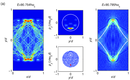
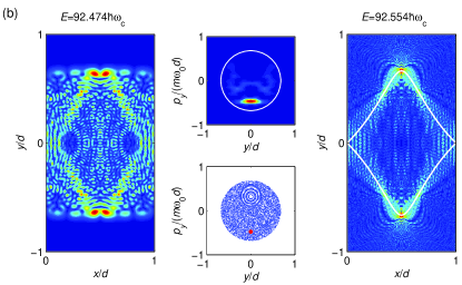
Figure 1: (Color). (a)-(d): Sequence of scarred wavefunctions localized around the bell-shaped unstable orbit in an electronic strip resonator with a parabolic longitudinal potential and a transverse magnetic field. Left panels: Color-coded modulus of the exact wavefunctions $|\Psi(x,y)|$ (blue: small amplitude, red: large amplitude). Right panels: The corresponding semiclassical ABL wavefunctions. The white curves depict the bell-shaped orbit, computed at the semiclassical energy. Upper middle panels: color-coded Husimi representations of the exact wavefunctions. Lower middle panels: classical phase space portraits, computed at the energy of the exact wavefunctions. The red dot denotes the position of the bell-shaped orbit. The white circle in the Husimi representations delimits the energetically accessible region of the classical phase space.

The classical dynamics of this system is of the generic, mixed, type, where stable orbits coexist with unstable orbits [see phase space portraits in the middle panels of Figs. 1(a)-(d)]. It was demonstrated previously for a similar system Zalipaev that the ABL method provides an accurate description of quantum states associated with stable orbits. Here we analyze an energy-dependent family of unstable bell-shaped orbits with two reflection points $(0,0)$ and $(d,0)$ at the hard walls [see white curves in the right panels of Figs. 1(a)-(d)]. The orbits consist of an upper and a lower arc, which are symmetrical to each other and are indexed in the following by $i=1,2$.

We solve the equation in variation (6) on each arc and then link these solutions together using a reflection matrix, which for non-vanishing magnetic field takes the form

$$R=\left(\begin{array}[]{cc}-1&0\\ -2\omega_{c}\tan\Theta&-1\end{array}\right),$$ (35)

where $\Theta$ is the angle of reflection. The monodromy matrix of the full orbit is found from the product $M=RM_{2}RM_{1}$, where $M_{i}$ is the fundamental matrix of arc $i$. There are eight singular points, where $z\overline{z}=0$: four well isolated focal points around $x\approx(0.5\pm 0.15)\,d$, $y\approx\pm 0.5\,d$, and two pairs of closely spaced focal points around $x\approx(0.5\pm 0.01)\,d$, $y\approx\pm 0.65\,d$. The stretching factor for the orbit (the largest eigenvalue of the monodromy matrix) is $\Lambda\approx 4.6$, corresponding to $\lambda\approx 1.53$.

Figure 2: Profile of the exact and semiclassical wave functions calculated along the line $y=0$. The width of the boundary layer where the ABL approach is valid is indicated in the upper left corner.

Semiclassically, the eigenstate is found as the sum of the two separatrix solutions (25) along each arc,

$$\Psi=\psi_{1}(z_{1},s,\nu)+r\psi_{2}(z_{2},s,\nu).$$ (36)

Here the coefficient $r$ follows from the continuity condition at the reflection points, and simply takes the value $r=-1$ for unstable orbits. The condition $\Psi=0$ at the boundaries $x=0$ and $x=d$ of the resonator can be taken into account by adopting a mirror reflection method BaKi ; BaBu . In this method, the wave function with the required boundary condition is obtained as the difference between the original solution and its mirror reflection at the boundary. In principle, the presence of the magnetic field requires to introduce an additional gauge field to eliminate the phase jump associated to the difference $\Gamma_{2}-\Gamma_{1}=2\omega_{c}$ entering the off-diagonal element of the reflection matrix Eq. (35). However, this affects only a small neighborhood $\propto\sqrt{\hbar}$ of the point of reflection.

In order to compare the resulting ABL solutions with exact quantum mechanics, we construct numerical eigenstates in an orthogonalized basis spanned by the exact solutions of the quasi-one dimensional system without the hard walls, which separates in the gauge ${\bf A}=-By{\bf e_{x}}$. The boundary conditions $\Psi(x=0,d;y)=0$ are imposed via a singular value decomposition (for details on such methods see, e.g., Ref. numerics ).

Our numerical computations reveal that the family of bell-shaped unstable orbits supports a long sequence of scarred wavefunctions, which are found at almost equidistantly spaced energies. Four consecutive examples (with longitudinal quantum numbers $n=66,67,68,69$) are shown in the left panels of Figs. 1(a)-(d). The corresponding ABL wavefunctions (right panels) accurately capture the typical spatial extent of the scar signature, including the position of the focal points, where the scar structure shrinks while the amplitude is significantly enhanced (close to the almost-degenerate pairs of focal points the wave function could be further regularized by adapting the general techniques of uniform approximations; see, e.g., Refs. Berry3 ; bifurcations ).

The clear correspondence between the exact quantum states and the ABL separatrix solutions is further confirmed by the Husimi representations $H(y,p_{y})=|\langle y,p_{y}|\partial_{x}\Psi(x=0,y)\rangle|^{2}$, which are obtained by overlapping the derivative of the exact wavefunction at the left wall with coherent states (minimal-uncertainty wave packets) that are parameterized in Birkhoff coordinates $y,p_{y}$. The Husimi representation, shown in the upper middle panels of Figs. 1(a)-(d), in all cases displays a clear maximum at the position of the bell-shaped orbit (red dot in the chaotic part of the phase-space portraits), which lies in the chaotic part of phase space.

Besides the visual agreement, the separatrix solutions also recover the following essential characteristics of the numerical solutions: (i) The wavefunctions are of the right symmetry with respect to inversion around $x=0.5\,d$, $y=0$ (as there are eight focal points, wavefunctions are symmetric under this operation when $n$ is odd, while they are antisymmetric when $n$ is even). (ii) The profile of the wave function along the line $y=0$ extracted from the ABL and the numerical solution (after spatial averaging over a range of $0.05\,d$ to eliminate the speckle fluctuations due to the random background in the numerical solution) shows a very good agreement within validity region of the ABL solution, $x/d\lesssim 0.15$. The ABL captures well both the period and the relative strength of the oscillations in the numerical solution. (iii) The exact energies are in excellent agreement with $E_{n_{0}}$, i.e., the semiclassical prediction from Eq. (22) with $\eta=0$. These energies are almost equidistantly spaced, and the semiclassical error is less than $5\%$ of this spacing (the error is also small compared to the mean level spacing of all states). (iv) For each longitudinal wavenumber $n$ the numerical computations only deliver a single scarred wavefunction localized around the unstable trajectory (in contrast, many transversely excited wavefunctions are supported by the stable trajectories in the island around $y\approx 0$, $p_{y}\approx 0.3\,m\omega_{0}d$). In other words, we do not find any other scarred states on this orbit. Therefore, the actual scar quantization window is reduced beyond the constraint obtained by the propagation of time dependent Gaussian states Heller3 , which predicts scarring in a larger window $\Delta E\approx\hbar\lambda_{T}$. However, one cannot exclude that signatures of off-resonant scarring show up in the wavefunction statistics of the states in this larger window, which is a question beyond our focus on individual wave functions.

VI Conclusions

In this work we extended the asymptotic boundary layer (ABL) method for semiclassical wave functions, originally developed for the description of Gaussian beams guided by stable trajectories, to the case of scar-like states localized in the vicinity of unstable periodic orbits. We focus on wavefunctions scarred by a single short trajectory and derive expressions of a universal form, valid up to order $\hbar^{3/2}$, which apply to general systems which may combine hard walls, external potentials and magnetic fields. The ABL equations are formulated in a curvilinear coordinate system associated with the classical trajectory. The system- and orbit-specific information enters via the solution of the classical equations in variations, which describe the stability of the trajectory. At fixed energy, the profile of the wavefunction is determined by a periodicity condition, which results in a Bohr-Sommerfeld quantization formula.

Far away from the guiding trajectory, the ABL wave function decays as the inverse square-root of the distance, and therefore is not normalizable, but couples to the quasi-random background of other modes in the system. This coupling is the weakest for the symmetric separatrix state, which is associated to a particulary simple quantization condition. Since the separatrix state is also the most visibly localized ABL wavefunction, one can expect that it typically provides the dominant contribution to scars guided by a single short trajectory. In general, we estimate that the number of wave functions of different profile participating in the scar formation increases logarithmically with the system dimensions, and therefore depends on the relation of the Ehrenfest time and the period of the trajectory.

We verified our conclusions by comparison with exact numerical solution for a quantum strip resonator with the quadratic confining potential and a perpendicular magnetic field. In this system, a family of unstable periodic orbits supports a long sequence of scarred states, with energies in excellent agreement with the simple quantization condition for the separatrix solution. We find that this solution captures all the essential characteristics of the exact scarred states. The studied system is of the generic type, with a mixed phase space, which raises the expectation that the ABL formalism is applicable to a large class of quantum-dynamical systems.

An open question concerns the generalization of the formalism to scars supported by many trajectories, as well as the contribution of ABL solutions to off-resonant scars (typically revealed in wavefunction statistics).

This work was supported by the European Commission via Marie-Curie excellence grant No. MEXT-CT-2005-023778.

Appendix A ABL expansion for Schrödinger equation

In this appendix we outline the main steps in the derivation of the ABL formalism. Further details on the formalism can be found in Refs. BaKi ; BaBu . Here, we present a straightforward derivation based on the direct expansion of the Schrödinger equation.

The main trajectory ${\bf r}_{0}(s)$, which is parameterized by its arclength $s$, generates an orthogonal coordinate system spanned by the normal unit vector ${\bf e}_{n}(s)$ and the longitudinal unit vector ${\bf e}_{t}(s)$, which we express in the component form

$${\bf e}_{n}(s)\equiv\left(\begin{array}[]{c}\gamma_{x}\\ \gamma_{y}\end{array}\right),~{}{\bf e}_{t}(s)\equiv\left(\begin{array}[]{c}\gamma_{y}\\ -\gamma_{x}\end{array}\right).$$ (41)

Recalling the conversion formulas for the partial derivatives in curvilinear coordinates,

$$\partial_{x}=\frac{\gamma_{y}}{\xi}\partial_{s}+\gamma_{x}\partial_{n},~{}\partial_{y}=-\frac{\gamma_{x}}{\xi}\partial_{s}+\gamma_{y}\partial_{n},$$ (42)

$$\xi=1-\frac{n}{\rho(s)},$$

where $\rho(s)$ is the curvature radius of the trajectory, we write the Schrödinger equation as

$$\frac{\Psi_{ss}}{\xi^{2}}-\frac{n\dot{\rho}}{\xi^{3}\rho^{2}}\Psi_{s}-\frac{\Psi_{n}}{\xi\rho}+\Psi_{nn}+\frac{i{eB}}{\hbar\xi}\left[({\bf r}_{0}{\bf e}_{n})+n\right]\Psi_{s}$$

$$+\frac{i{eB}}{\hbar}({\bf r}_{0}{\bf e}_{l})\Psi_{n}-\frac{{e^{2}B}^{2}}{4\hbar^{2}\xi^{3}}({\bf r}_{0}+{\bf e}_{n}n)^{2}\Psi=\frac{2m}{\hbar^{2}\xi^{3}}(U-E)\Psi,$$ (43)

where $U(s,n)$ is the potential inside the resonator.

The central idea of the ABL approach is to search the solution to Eq.  (43) in an asymptotically small boundary layer of the width $\propto\sqrt{\hbar}$ in the vicinity of the main trajectory. A straightforward way to derive the corresponding semiclassical expansion for the wave function follows two steps: (i) scaling the normal variable as $n=\sqrt{\hbar}\nu$ and (ii) expanding the resulting equation in powers of $\sqrt{\hbar}$, as written in Eq. (1), where each term $\psi^{(j)}$ is uniquely defined.

We substitute Eq. (1) into Eq.  (43), expand the resulting equation, and match the coefficients of the resulting series, which yields a hierarchical set of equations for $S_{0}(s)$, $S_{1}(s)$, and $\psi^{(j)}(s,\nu)$. If the expansion of the effective potential can limited to second order (a standard assumption in linear scar theories Kaplan ; Dambrowsky ), one can terminate the series in Eq. (1) at the leading term $\psi^{(0)}(s,\nu)$. This is equivalent to obtaining a semiclassical wave function to the order of $\hbar^{3/2}$ BaKi . The first three terms of the series expansion of Eq. (43) read

$$\hbar^{-2}: {\cal A}\ \psi^{(0)}=0,$$ (44a)

$$\hbar^{-3/2}: {\cal A}\ \psi^{(1)}+2i{\cal B}\ \psi^{(0)}_{\nu}+{\cal C}\nu\ \psi^{(0)}=0,$$ (44b)

$$\hbar^{-1}: {\cal C}\nu\ \psi^{(1)}+2i{\cal B}\ \psi^{(1)}_{\nu}+{\cal D}=0,$$ (44c)

with coefficients

$${\cal A} =a^{2}-\frac{r_{0}^{2}{e^{2}B}^{2}}{4}-{eB}({\bf r}_{0}{\bf e}_{l})S_{1}-S_{1}^{2}+{eB}({\bf r}_{0}{\bf e}_{n}){\dot{S}}_{0}-{\dot{S}}_{0}^{2},$$ (45a)

$${\cal B} =\frac{eB}{2}({\bf r}_{0}{\bf e}_{l})+S_{1},$$ (45b)

$${\cal C} =\frac{S_{1}^{2}-{\dot{S}}_{0}^{2}}{\rho}-2{\dot{S}}_{0}{\dot{S}}_{1}-eB{\dot{S}}_{0}^{2}-eB{\dot{S}}_{1}({\bf r}_{0}{\bf e}_{n})$$

$$-\frac{eB}{\rho}({\bf r}_{0}{\bf e}_{l})S_{1}-2mu_{1}-\frac{a^{2}}{\rho}+\frac{e^{2}B^{2}}{4\rho}r_{0}^{2}-\frac{e^{2}B^{2}}{2}({\bf r}_{0}{\bf e}_{n}),$$ (45c)

$${\cal D} =2ia\ {\dot{\psi}}^{(0)}+i{\dot{a}}\ \psi^{(0)}+\psi^{(0)}_{\nu\nu}-da^{2}\nu^{2}\ \psi^{(0)}.$$ (45d)

Equation (44a) yields ${\cal A}=0$. Equation (44b) is solved by setting ${\cal B}=0$, since ${\cal C}=0$ is satisfied identically if ${\cal A}={\cal B}=0$, which yields the classical action solution (2). Finally Eq. (44c) is equivalent to ${\cal D}=0$, which yields Eq. (3). After the substitution $\phi=a^{-1/2}\psi^{(0)}$ this equation take the form of a nonstationary Schrödinger equation, which we write as

$$\hat{L}\phi\equiv\left\{i\partial_{s}+\frac{\partial_{\nu}^{2}}{2a}-\frac{ad}{2}\nu^{2}\right\}\phi=0.$$ (46)

The fact that Eq. (5) is a solution to Eq. (3) can be checked by a direct substitution. Here we present a direct derivation, which provides deeper insight into the nature of the ABL solution. First, we obtain a “ground state” solution to Eq. (46) by using the ansatz

$$\phi_{0}=\mu(s)\exp\left\{i\ \frac{\Gamma(s)}{2}\ \nu^{2}\right\},$$ (47)

which is similar to the thawed Gaussians introduced by Heller Heller_g to describe the time evolution of localized quantum wave packets. Substituting Eq. (47) into Eq. (46) yields equations for the unknown quantities $\Gamma$ and $\mu$,

$$\dot{\Gamma}+\frac{\Gamma^{2}}{a}+ad=0,$$ (48a)

$$\mu=\exp\left\{-\frac{1}{2}\int_{0}^{s}\frac{\Gamma}{a}ds\right\}.$$ (48b)

The Ricatti equation (48a) is solved by a standard substitution $\Gamma=p/z$, after which one finds equations for $p$ and $z$ as given by Eq. (6). As we mentioned above, this Hamiltonian equations in variations define relative coordinates $z$ and momentum $p$ for classical trajectories in the vicinity of the guiding trajectory. Once Eq. (6) is solved, Eq. (48b) delivers $\mu=z^{-1/2}$. Equation (6) has two linearly independent solutions, $(z,p)$ and $({\overline{z}},{\overline{p}})$, which define the constant Wronskian $p{\overline{z}}-{\overline{p}}z=w$.

The classical origin of Eq. (6) can be established from the reduced classical action constructed for the trajectory $n(s)$ in the vicinity of the guiding trajectory. In curvilinear coordinates this action reads

$$S=\int_{0}^{s}\sqrt{2m(E-U(r))}\left\{\left(1-\frac{n}{\rho}\right)^{2}+{\dot{n}}^{2}\right\}^{1/2}ds$$

$$+\frac{eB}{2}\int_{0}^{s}\left(x\dot{y}-y\dot{x}\right)ds,$$ (49)

where $x=x_{0}(s)+\gamma_{x}(s)n(s)$ and $y=y_{0}(s)+\gamma_{y}(s)n(s)$. Expanding Eq.  (49) to second order in the small quantity $n$, one obtains

$$S=S_{0}-\int_{0}^{s}\varepsilon\ n\ ds+\frac{1}{2}\int_{0}^{s}\left(a\dot{n}^{2}-adn^{2}\right)ds,$$ (50)

where

$$\varepsilon(s)={eB}+\frac{a}{\rho}+\frac{au_{1}}{2(E-u_{0})}.$$ (51)

The linear term in this expansion vanishes identically, $\varepsilon=0$, because $n=0$ is also a trajectory (the main trajectory). The linear coefficient in Eq. (50) is related to Eq. (45) as ${\cal C}=2a\varepsilon$, which explains why ${\cal C}$ vanishes. The Euler-Lagrange equation for the action (50) is equivalent to the Hamiltonian system (6).

A sequence of partial solutions to Eq.  (3) can be constructed with the help of creation and annihilation operators Mas1 ; BaKi

$$\hat{\Lambda}=\sqrt{\frac{i}{w}}\left(-i\ z\ \partial_{\nu}-p\ \nu\right),$$ (52a)

$$\hat{\Lambda}^{\dagger}=\sqrt{\frac{i}{w}}\left(-i\ {\overline{z}}\ \partial_{\nu}-{\overline{p}}\ \nu\right),$$ (52b)

which satisfy the following algebra

$$[\hat{\Lambda},\hat{L}]=[\hat{\Lambda}^{\dagger},\hat{L}]=0,\ [\hat{\Lambda},\hat{\Lambda}^{\dagger}]=1.$$ (53)

General solutions are then obtained from $\psi_{m}=\Lambda^{\dagger m}\psi_{0}$. This procedure leads to a recurrence relation, which is solved by wave functions of the explicit form

$$\phi_{m}(s,\nu)\propto\frac{{\overline{z}}^{m}(\Gamma-{\overline{\Gamma}})^{m/2}}{\sqrt{z}}H_{m}\left(\sqrt{\frac{\Gamma-{\overline{\Gamma}}}{2i}}~{}\nu\right)e^{\frac{i}{2}\Gamma\nu^{2}},$$ (54)

where $H_{m}$ are Hermite polynomials.

The presented derivation allows for an unambiguous analytical continuation of the recurrence relation and its solutions to arbitrary indices $m\rightarrow\xi$. This yields Eq. (5), where the parabolic cylinder functions $D_{\xi}$ take the place of the Hermite polynomials $H_{m}$, and the coefficient $a^{-1/2}$ is accounted for. Finally, we note that recalling the definition of $\Gamma$ and $\overline{\Gamma}$ as well as that for the Wronskian, the solution can be compactly written as

$$\phi_{\xi}(s,\nu)\propto\frac{e^{\frac{i}{4}(\Gamma+\overline{\Gamma})\nu^{2}}}{\sqrt{z}}\left(\frac{\overline{z}}{z}\right)^{\xi/2}D_{\xi}\left(\sqrt{\frac{w}{iz\overline{z}}}~{}\nu\right).$$ (55)

References

- (1) V. M. Babich and N. Ya. Kirpichnikova, The boundary-layer method in diffraction problems (Springer, Berlin, 1979).
- (2) V. M. Babich and V. S. Buldyrev, Asymptotic methods in shortwave diffraction problems (Springer, Berlin, 1991).
- (3) V. V. Belov and S. Yu. Dobrokhotov, Sov. Math. Doclady 37, 264 (1988).
- (4) V. V. Zalipaev, F. V. Kusmartsev, and M. M. Popov, J. Phys. A: Math. Theor. 41, 065101 (2008).
- (5) H. J. Stöckmann, Quantum Chaos. An Introduction (Cambridge University Press, Cambridge, 2000).
- (6) M. V. Berry, J. Phys. A: Math. Gen. 10, 2083 (1977).
- (7) A. Voros, in Stochastic Behaviour in Classical and Quantum Hamiltonian Systems, ed. G. Casati and G. Ford (Berlin, Spinger, 1979).
- (8) E. J. Heller, Phys. Rev. Lett. 53, 1515 (1984).
- (9) L. Kaplan and E. J. Heller, Ann. Phys. 264, 171 (1998).
- (10) S. Sridhar, Phys. Rev. Lett. 67, 785 (1991).
- (11) P. B. Wilkinson, T. M. Fromhold, L. Eaves, F. W. Sheard, N. Miura, and T. Takamasu, Nature (London) 380, 608 (1996).
- (12) N. B. Rex, H. E. Tureci, H. G. L. Schwefel, R. K. Chang, and A. D. Stone, Phys. Rev. Lett. 88, 094102 (2002); S.-B. Lee, J.-H. Lee, J.-S. Chang, H.-J. Moon, S. W. Kim, and K. An, Phys. Rev. Lett. 88, 033903 (2002); C. Gmachl, E. E. Narimanov, F. Capasso, J. N. Ballargeon, and A. Y. Cho, Opt. Lett. 27, 824 (2002); T. Harayama, T. Fukushima, P. Davis, P. O. Vaccaro, T. Miyasaka, T. Nishimura, and T. Aida, Phys. Rev. E 67, 015207(R) (2003).
- (13) T. M. Antonsen, E. Ott, Q. Chen, and R. N. Oerter, Phys. Rev. E 51, 111 (1995).
- (14) K. Damborsky and L. Kaplan, Phys. Rev. E 72, 066204 (2005).
- (15) E. G. Vergini, J. Phys. A: Math. Gen. 33, 4709 (2000); E. G. Vergini and G. G. Carlo, J. Phys. A: Math. Gen. 33, 4717 (2000); E. G. Vergini and G. G. Carlo, J. Phys. A: Math. Gen. 34, 4525 (2001).
- (16) M. Novaes, J. M. Pedrosa, D. Wisniacki, G. G. Carlo, and J. P. Keating, arXiv:0906.1552 (2009).
- (17) E. B. Bogomolny, Physica D 31, 169 (1988).
- (18) M. V. Berry, Proc. R. Soc. London A 243, 219 (1989).
- (19) O. Agam and S. Fishman, Phys. Rev. Lett. 73, 806 (1994).
- (20) L. Kaplan, Phys. Rev. Lett. 80, 2582 (1998).
- (21) S. Nonnenmacher and A. Voros, J. Phys. A 30, 295 (1997).
- (22) R. V. Mendes, Phys. Lett. A 239, 223 (1998).
- (23) S.-Y. Lee and S. C. Greagh, Ann. Phys. 307, 392 (2003).
- (24) T. M. Fromhold, P. B. Wilkinson, F. W. Sheard, L. Eaves, J. Miao, and G. Edwards, Phys. Rev. Lett. 75, 1142 (1995).
- (25) E. J. Heller, J. Chem. Phys. 62, 1544 (1975).
- (26) N. Anantharaman and S. Nonnenmacher, Annales de l’Institut Fourier 57, 2465 (2007); N. Anantharaman, H. Koch, and S. Nonnenmacher, arXiv:0704.1564; B. Gutkin, arXiv:0802.3400v1.
- (27) H. Schomerus and J. Tworzydło, Phys. Rev. Lett. 93, 154102 (2004).
- (28) J. P. Keating, M. Novaes, S. D. Prado, and M. Sieber, Phys. Rev. Lett. 97, 150406 (2006).
- (29) G. M. Zaslavsky, Phys. Rep. 80, 157 (1981); I. L. Aleiner and A. I. Larkin, Phys. Rev. B 54, 14423 (1996); H. Schomerus and Ph. Jacquod, J. Phys. A: Math. Gen. 38, 10663 (2005).
- (30) V. P. Maslov and M. V. Fedoriuk, Semiclassical approximation in quantum mechanics (Reidel, Dordrecht, 1981).
- (31) M. V. Berry, J. Phys.: Math. Gen. 10, 2061 (1977).
- (32) M. V. Berry, J. P. Keating, and H. Schomerus, Proc. R. Soc. London A 456, 1659 (2000); J. P. Keating and S. Prado, Proc. R. Soc. London A 457, 1855 (2001).
- (33) A. Bäcker, Lect. Notes Phys. 618, 91 (2003).
- (34) L. Kaplan and E. J. Heller, Phys. Rev. E 59, 6609 (1999).