Implementation of Fault Tolerant Quantum Logic Gates via Optimal Control

Abstract

The implementation of fault-tolerant quantum gates on encoded logic qubits is considered. It is shown that transversal implementation of logic gates based on simple geometric control ideas is problematic for realistic physical systems suffering from imperfections such as qubit inhomogeneity or uncontrollable interactions between qubits. However, this problem can be overcome by formulating the task as an optimal control problem and designing efficient algorithms to solve it. In particular, we can find solutions that implement all of the elementary logic gates in a fixed amount of time with limited control resources for the five-qubit stabilizer code. Most importantly, logic gates that are extremely difficult to implement using conventional techniques even for ideal systems, such as the $T$-gate for the five-qubit stabilizer code, do not appear to pose a problem for optimal control.

1 Introduction

Quantum information processing has been a topic of intense theoretical and experimental research for several years. Many potential physical realizations of quantum computers have been proposed, and although the experimental realization of quantum information processing remains a challenge, there have been many experimental accomplishments including the demonstration of control of multi-qubit dynamics in spin systems using nuclear magnetic resonance techniques [1] and all-optical quantum information processing using photons [2], for instance. While liquid-state NMR and optical quantum computing may suffer from inherent scalability issues, there has also been significant progress in ion-trap architectures and several proposals for making such architectures scalable exist [3, 4]. In solid-state systems successes have been more modest but controlled interactions of quantum dots have been demonstrated in some systems [5, 6].

One major obstacle to scalability is the increasing difficulty in effectively controlling the dynamics of many qubits as the complexity of experimental systems increases. While it is in principle easy to control a single two-level system, the situation is more complicated when many qubits are involved. In many cases individual addressability of qubits in a register or array is difficult to achieve; inhomogeneity may result in different qubits having different responses to control fields, and the dynamics is complicated by uncontrollable inter-qubit couplings. All of these issues present challenges, even in the absence of environmental noise and decoherence. These problems are magnified because the necessity to be able to correct at least a certain amount of inevitable errors means that bits of quantum information must be encoded in logical qubits consisting of multiple physical qubits to ensure that there is sufficient redundancy. Even if only the most basic level of protection is assumed, at least five physical qubits are required to encode a single logical qubit so that we can correct a single (bit or phase flip) error [10]. In practice multiple layers of error correction will be necessary to achieve fault-tolerant operation of a quantum processor for a sufficiently long time to allow the completion of a non-trivial quantum algorithm [10]. Thus, in the setting of fault-tolerant computation using encoded qubits even the implementation of single qubit logic gates becomes a non-trivial multi-qubit control problem.

The implementation of fault-tolerant gates quantum logic gates seems to be a problem that is well suited for optimal control. Optimal control theory has been used in various papers to implement two and three qubit gates as well as simple quantum circuits, and has been shown to improve gate fidelities, gate operation times and robustness (e.g. [7, 8, 9]). In this paper we consider the implementation of logic gates on encoded qubits, which is a next logical step. Although most logic gates on encoded qubits for the most common codes can be implemented, in principle, by applying a particular single qubit operation to all physical qubits, what is known as transversal implementation, not all logic gates can be implemented this way even in the ideal case, and transversal implementation is problematic in the presence of inhomogeneity or uncontrollable couplings between physical qubits, and the implementation of encoded logic gates in this setting is therefore in an interesting challenge for optimal control. In particular we study the implementation of a set of logic gates for the five-qubit stabilizer code for model systems with both inhomogeneity and fixed inter-qubit couplings. The paper is organized as follows. In Sec. 2 we briefly introduce stabilizer codes and the construction of fault-tolerant logic gates with emphasis on the five-qubit stabilizer code that will be the main focus of this paper. In Sec. 3 we describe two types of model systems and discuss the implementation of encoded logic gates for these system based on geometric control ideas. In section 4 we formulate the optimal control problem and show how to design iterative algorithms to solve it numerically. In Sec. 5 the results are applied to find optimal controls to implement a set of standard logic gates for the five-qubit stabilizer code for two classes of model systems, and the merits and drawback of the optimal control approach compared with the simpler geometric control schemes are discussed.

2 Stabilizer codes and fault-tolerant gates

The state of a single qubit can be represented by a density operator $\rho$ on a Hilbert space $\mathcal{H}\simeq\mathbb{C}^{2}$, which can be expanded with respect to the standard Pauli basis, $\rho=\frac{1}{2}(\mathbb{I}+x\sigma_{x}+y\sigma_{y}+z\sigma_{z})$, where $\mathbb{I}$ is the identity matrix and

$$\sigma_{x}=\left(\begin{array}[]{cc}0&1\\ 1&0\end{array}\right),\quad\sigma_{y}=\left(\begin{array}[]{cc}0&-i\\ i&0\end{array}\right),\quad\sigma_{z}=\left(\begin{array}[]{cc}1&0\\ 0&-1\end{array}\right).$$ (1)

are the usual Pauli matrices, and we have $*=\Tr(\sigma_{*}\rho)$ for $*\in\{x,y,z\}$. Any single qubit gate can be written

$$R_{\hat{\bf n}}(\alpha)=\exp\left(i\frac{\alpha}{2}\,\hat{\bf n}\cdot{\bm{\sigma}}\right),$$ (2)

where ${\bm{\sigma}}=(\sigma_{x},\sigma_{y},\sigma_{z})$, which can be interpreted as a rotation of the Bloch vector ${\bf s}=(x,y,z)\in\mathbb{R}^{3}$ by an angle $\alpha$ around the axis $\hat{\bf n}=(n_{x},n_{y},n_{z})$. We further note that the norm of the Bloch vector $\|{\bf s}\|\leq 1$, with equality if and only if $\rho$ represents a pure state.

The ability to implement universal quantum operations on $n$ qubits requires a minimal set of elementary gates, which typically comprises several essential single qubit gates such as the identity $\mathbb{I}$, the $S$ and $T$ gates and the Hadamard gate

$$S=R_{\hat{\bf z}}\left(\frac{\pi}{2}\right),\quad T=R_{\hat{\bf z}}\left(\frac{\pi}{4}\right),\quad\mbox{\rm Had}=R_{\hat{\bf n}}(\pi),$$ (3)

where $\hat{\bf n}=\frac{1}{\sqrt{2}}(1,0,1)$, and a single universal two-qubit gate such as the CNOT gate [10]. Often the $\pi$-rotations about the $x$, $y$ and $z$-axis, $X=\sigma_{x}$, $Y=\sigma_{y}$, $Z=\sigma_{z}$, respectively, are also included for convenience.

To protect quantum information from errors due to noise and decoherence several physical qubits are required to encode a logical qubit in a way that enables us to recover quantum information from corrupted qubits. Different types of encodings exists to protect against different types of errors, but the most common encodings are decoherence-free subspaces and stabilizer codes [10]. In this paper we focus on the latter type of encoding, where errors can be corrected by performing (projective) syndrome measurements on encoded qubits and applying the correcting quantum gates to the corrupted qubit. The minimum number of physical qubits required to encode a single quantum bit of information such that we can recover from a single bit or phase flip error on any of the physical qubits is the five-qubit stabilizer code based on the encoding

$$\ket{0_{L}} = \frac{1}{4}[\ket{00000}+\ket{10010}+\ket{01001}+\ket{10100}$$ (4)

$$+\ket{01010}-\ket{11011}-\ket{00110}-\ket{11000}$$

$$-\ket{11101}-\ket{00011}-\ket{11110}-\ket{01111}$$

$$-\ket{10001}-\ket{01100}-\ket{10111}-\ket{00101}]$$

$$\ket{1_{L}} = \frac{1}{4}[\ket{11111}+\ket{01101}+\ket{10110}+\ket{01011}$$ (5)

$$+\ket{10101}-\ket{00100}-\ket{11001}-\ket{00111}$$

$$-\ket{00010}-\ket{11100}-\ket{00001}-\ket{10000}$$

$$-\ket{01110}-\ket{10011}-\ket{01000}-\ket{11010}],$$

where $\ket{00\ldots}$ is the usual shorthand for the tensor product $\ket{0}\otimes\ket{0}\otimes\ldots$. Thus, a single qubit logic gate on encoded qubits is equivalent to a five-qubit gate represented by a $32\times 32$ unitary matrix. There is a certain degree of freedom in the definition of logic gates but a logic $X$-gate, for instance, must obviously swap the logic states $\ket{0_{L}}$ and $\ket{1_{L}}$. Moreover, the key premise of fault-tolerant logic gate construction is that the application of a particular logic gate to a corrupted qubit, should not increase the number of errors. Thus, an encoded qubit corrupted by a single bit or phase flip error on a physical qubit must be mapped to a state with a single bit or phase flip error to enable subsequent error correction. If $X_{n}$ is denotes a bit flip applied to the $n$th qubit then the requirement of unitarity prevents us from directly correcting errors as we cannot map both $\ket{0_{L}}$ and the corrupted state $X_{n}\ket{0_{L}}$ to $\ket{1_{L}}$. With this in mind, it is straightforward to derive suitable matrix representations for the fault-tolerant gates. For example, the logical $X_{L}$ gate must map $\ket{0_{L}}$ to $\ket{1_{L}}$ and vice versa. Furthermore, an input state corrupted by a single bit flip error on the $n$th qubit, $X_{n}\ket{0_{L}}$ should be mapped to the output state $X_{n}\ket{1_{L}}$, i.e., the target state $\ket{1_{L}}$ with a bit flip on the $n$th qubit, or more generally

$$X_{L}=\ket{1_{L}}\bra{0_{L}}+\sum_{n>m}[X_{n}\ket{1_{L}}\bra{0_{L}}X_{n}+X_{n}X_{m}\ket{1_{L}}\bra{0_{L}}X_{m}X_{n}]+c.c.$$ (6)

where $c.c.$ denotes the complex conjugate. The same relationship between the input and output states should hold when the bit flip errors $X_{n}$ are replaced by phase flip errors $Z_{n}$. This fully determines the logic $X_{L}$ gate. We can similarly derive explicit representations for all other logic gates. Fig. 1 shows the structure of the resulting unitary operators corresponding to the target gates.

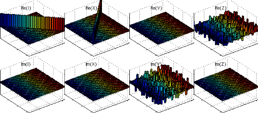
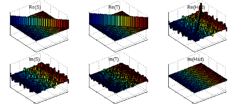
Figure 1: Real and imaginary parts of $32\times 32$ unitary operators corresponding to the encoded logic gates.

Given a register of identical and non-interacting qubits, most fault-tolerant quantum logic gates can be implemented transversally, i.e., by applying the same single qubit operation in parallel to each qubit in the register. For instance, it is can easily be verified that the logical $X$-gate defined by (6) is simply $X_{L}=X\otimes X\otimes X\otimes X\otimes X$, i.e., an $X$ gate applied to each physical qubit, However, even if we are given ideal non-interacting physical qubits, not all quantum logic gates can be implemented transversally. For instance, the $T$-gate above, which is required for universality, cannot be realized this way. Indeed, implementation of the $T$-gate for the five-qubit code above is generally complicated, requiring auxiliary qubits and quantum teleportation [10]. Furthermore, for real physical systems inhomogeneity and uncontrollable interactions may make simple transverse implementation of fault-tolerant gates impractical, if not impossible.

3 Model systems and geometric control schemes

Quite a few proposed realizations for quantum computing architectures can be formally thought of as linear arrays of two-level systems (qubits or pseudo-spin-$\frac{1}{2}$-particles). In the ideal case one usually considers individual spins that are identical, individually addressable and controllable, and assumes the couplings between all qubits are fully controllable. In practice, however, these requirements are difficult to meet as the coupling between spins is often not controllable, and the qubits may not be identical or selectively addressable. In this case simple transverse implementation of quantum logic gates is not possible even for simple gates such as the $X$-gate, and an optimal control approach seems the most promising way to overcome such obstacles to implement quantum logic gates with limited control.

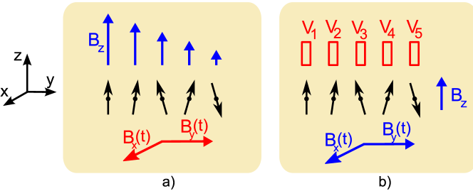
Figure 2: Spin chain controlled (a) by modulation of global fields and (b) using a fixed global field and local electrodes that tune individual qubits in and out of resonance with the field. $B_{x}(t)$, $B_{y}(t)$ and $B_{z}(t)$ indicate the $x$, $y$ and $z$ components of a globally applied field. $V_{k}$ refer to control parameters for local actuators, e.g., voltages applied to control electrodes.

In the following we consider two control paradigms (a) global control and (b) limited local control, as shown in Fig. 2. In case (a) the physical qubits comprising the logic qubit are controlled entirely by a global field that interacts with all physical qubits simultaneously. In case (b) there may also be a fixed global field but the actual control operations are performed using local control gates, such as local control electrodes that tune individual spins in and out of resonance with a global field.

3.1 Global Control

If the qubits are identical and there are no couplings between them, then transversal logic gates can be easily implemented in the global control setting by simply finding a control pulse that implements the desired gate for a single qubit and applying it to all physical qubits. The elementary single qubit gates can be implemented, e.g., by applying a sequence of simple pulses effecting rotations about two orthogonal axes, using the Euler decomposition

$$R_{\hat{\bf n}}(\theta)=R_{\hat{\bf x}}(\alpha)R_{\hat{\bf y}}(\beta)R_{\hat{\bf x}}(\gamma)$$ (7)

for suitably chosen values of $\alpha,$ $\beta$ and $\gamma$, as shown in Table 1. Rotations about the $x$- or $y$-axis can be performed by applying a pulse of the form $f(t)=B(t)\cos(\omega t+\phi)$ with suitable frequency $\omega$, pulse area $\int_{t_{0}}^{t_{F}}B(t)\,dt$ and phase $\phi$ [9].

Gate	Euler decomposition	Pulse length
X	$R_{\hat{\bf x}}(\pi)$	1
Y	$R_{\hat{\bf y}}(\pi)$	1
Z	$R_{\hat{\bf x}}(\pi)R_{\hat{\bf y}}(\pi)$	2
I	$R_{\hat{\bf x}}(2\pi)$	2
S	$R_{\hat{\bf x}}(3\pi/2)R_{\hat{\bf y}}(\pi/2)R_{\hat{\bf x}}(\pi/2)$	2.50
T	$R_{\hat{\bf x}}(3\pi/2)R_{\hat{\bf y}}(\pi/4)R_{\hat{\bf x}}(\pi/2)$	2.25
Had	$R_{\hat{\bf y}}(\pi/2)R_{\hat{\bf x}}(\pi)$	1.50

Table 1: Euler decomposition of elementary gates in terms of rotations about $\hat{\bf x}$ and $\hat{\bf y}$ axis and total pulse length in units of $2\Omega/\pi$, where $\Omega$ is the effective (average) Rabi frequency of the pulse.

The problem becomes more complicated when the physical qubits are not exactly identical, i.e., when there is inhomogeneity resulting in the qubits having slightly different resonance frequencies, for instance. In this case we can switch to frequency-selective addressing, i.e., try to implement rotations on individual physical qubits by applying frequency-selective geometric pulse sequences in resonance with each qubit, either sequentially or concurrently. However, the pulse amplitudes (Rabi frequencies) have to be much smaller than the frequency detuning between the different qubits in this case to avoid off-resonant excitation effects. For instance, consider the system $H[f(t)]=H_{0}+f(t)H_{1}$ with

$$H_{0}=-\frac{\hbar}{2}\sum_{n=1}^{5}\omega_{n}\sigma_{z}^{(n)},\quad H_{1}=\frac{\hbar}{2}\sum_{n=1}^{5}\sigma_{x}^{(n)},$$ (8)

where $f(t)=\frac{\gamma_{n}}{2}B_{x}(t)$ and $\sigma_{z}^{(n)}$ ($\sigma_{x}^{(n)}$) denotes a five-fold tensor product, whose $n$th factor is $\sigma_{z}$ ($\sigma_{x}$) and all others are the identity $\mathbb{I}$, e.g., $\sigma_{z}^{(2)}=\mathbb{I}\otimes\sigma_{z}\otimes\mathbb{I}\otimes\mathbb{I}\otimes\mathbb{I}$. We can implement a logic $X$-gate by concurrently applying five Gaussian $\pi$-pulses

$$f_{n}(t)=q\sqrt{\pi}e^{-q^{2}(t-t_{n}/2)^{2}}\cos(\omega_{n}t),$$ (9)

i.e., choosing $f(t)=\sum_{n=1}^{5}f_{n}(t)$, where $\omega_{n}$ are the resonant frequencies $\{6,8,10,12,14\}$ above. $t_{n}$ is the length of the $n$th pulse. If the pulses have equal lengths and are applied concurrently then $t_{n}=t_{F}$ for all $n$. We can also apply the pulses sequentially but this significantly increases the total gate operation time as $t_{F}=\sum_{n}t_{n}$ in this case, and we will not consider this case here.

We can quantify the gate fidelity modulo global phases as the overlap of the actual gate implemented $U(t_{F})$ with the target gate $W$,

$$|\mathcal{F}_{W}(U(t_{F}))|=\frac{1}{N}|\Tr[W^{\dagger}U(t_{F})]|,$$ (10)

where the factor $\frac{1}{N}$, $N=\dim\mathcal{H}$, is a normalization factor included to ensure that $|\mathcal{F}|$ varies from $0$ to $1$, with unit fidelity corresponding to a perfect gate. For the model system above simulations suggest that we require at least approximately $t_{F}=440$ time units for Gaussian pulses with $q=0.01$ to achieve $>99.99$% fidelity.

Fig. 3 shows that the frequency-selective pulses perform as expected if the qubits are non-interacting. The control performs poorly, however, if non-zero couplings between adjacent physical qubits are present, e.g., if we add a simple uniform Ising coupling term

$$H_{I}=\hbar J\sum_{n=1}^{4}\sigma_{z}^{(n)}\sigma_{z}^{(n+1)}$$ (11)

between neighboring qubits, then the fidelity drops from $99.99$% for $J=0$ to $99.78$% for $J=0.0001$, to $86.90$% for $J=0.001$, to $26.97$% for $J=0.01$. Thus, even if the Ising coupling frequency $J$ is four orders of magnitude smaller than the median transition frequency $\omega=10$, the simple geometric pulse sequence becomes ineffective. This can be attributed to the creation of entanglement between the physical qubits over the duration of the pulse. The evolution of the five physical qubits on the Bloch sphere under the five concurrent $\pi$-pulses in Fig. 4 shows that the presence of the couplings completely changes the dynamics. In the absence of couplings the composite Gaussian pulse achieves the desired simultaneous bit flip for all the qubits, but in the presence of even moderate Ising couplings between adjacent qubits the pulse sequence becomes ineffective. A plot of the length of the Bloch vectors (Fig. 5) for $J=0.01$ shows a marked decrease for all qubits, indicating the development of significant entanglement between the qubits. Due to the nature of the couplings (Ising-type) the development of entanglement is not immediate. If we start in the product state $\ket{00000}$ then the effect of the couplings is felt only after sufficient coherence has been created by the pulse. The product state $\ket{00000}$ was chosen as an initial state, although it is not a logic state of the stabilizer code, because it serves well to illustrate the dynamics of the driving system.

Figure 3: A field composed of five concurrent Gaussian $\pi$-pulses with frequencies $\{6,8,10,12,14\}$ achieves a logic $X$-gate in the absence of interqubit coupling ($J=0$) but it is ineffective, for $J=0.01$, achieving a maximum fidelity $|\mathcal{F}|$ of only 27%. The high-frequency oscillations of the fields and fidelity are due to both being computed and shown in the stationary laboratory frame (no approximations) rather than in a multiply-rotating frame.

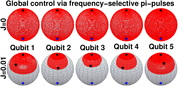
Figure 4: Trajectories (red) traced out by the Bloch vectors of the individual qubits on the Bloch sphere subject to the five concurrent $\pi$-pulses above for $J=0$ (top) and $J=0.01$ (bottom). ($\bullet$ initial state, $\bigstar$ final state, $\tiny{\color[rgb]{0,0,1}\blacksquare}$ target final state (south pole)

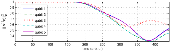
Figure 5: Length of the Bloch vectors ${\bf s}^{(n)}(t)$ of the five physical qubits as a function of time for $J=0.01$. Its decrease is evidence of the formation of entanglement between the individual qubits.

3.2 Local control

The second control paradigm we consider local control through selective detuning of individual dots in a quantum register via local voltage gates, as recently considered, e.g., in [11]. The individual qubits here are subject to a fixed, global magnetic field ${\bf B}(t)$ as well as local voltage gates that allows us to control the energy level splitting $\omega_{n}$ of each of the qubits. If there is no coupling between qubits, setting ${\bf B}(t)=B(\cos\omega t,-\sin\omega t,B_{z})$ leads to a Hamiltonian of the form

$$H=\frac{\hbar}{2}\sum_{n}\gamma_{n}B[\cos(\omega t)\sigma_{x}^{(n)}-\sin(\omega t)\sigma_{y}^{(n)}]+\frac{\hbar}{2}\sum_{n}\omega_{n}({\bf V}(t))\sigma_{z}^{(n)}$$ (12)

where $\omega_{n}({\bf V})$ indicates that the dependence of the energy level splitting $\omega_{n}$ of the $n$th on external control voltages ${\bf V}$. It is convenient in this case to transform to a moving frame $U_{0}(t)=\exp(it\omega\frac{1}{2}\sum_{n}\sigma_{z}^{(n)})$ rotating at the field frequency $\omega$, in which the Hamiltonian takes the form

$$H=\hbar\Omega\sum_{n}\sigma_{x}^{(n)}+\hbar\sum_{n}u_{n}(t)\sigma_{z}^{(n)},$$ (13)

if we set $\Omega=\frac{1}{2}B\gamma_{0}$ and $u_{n}(t)=\frac{1}{2}\Delta\omega_{n}({\bf V}(t))$ with $\Delta\omega_{n}({\bf V}(t))=\omega_{n}({\bf V}(t))-\omega$, and for simplicity assume $\gamma_{n}=\gamma_{0}$ for all $n$. In the following we do not consider the architecture-specific functional dependence of resonant frequencies on the gate voltages ${\bf V}$ and cross-talk issues [12, 13] and take ${\bf u}(t)=(u_{1}(t),u_{2}(t),\ldots,u_{5}(t))$ to be independent controls.

In the absence of interactions, it is again relatively straightforward to implement arbitrary rotations on any qubit using a simple geometric control design. We can clearly perform simultaneous rotations about the $\hat{\bf x}$-axis on all physical qubits simply by choosing the detuning parameters $u_{n}(t)=0$. To rotate qubits about the $\hat{\bf y}$-axis we can make use of the following result [11]

$$R_{\hat{\bf y}}(4\phi)=R_{\hat{\bf x}}(\pi)R_{\hat{\bf n}}(\pi)R_{\hat{\bf x}}(\pi)R_{\hat{\bf n}}(\pi),$$ (14)

where $R_{\hat{\bf x}}(\pi)$ is a $\pi$ rotation about the $\hat{\bf x}$-axis and $R_{\hat{\bf n}}(\pi)$ is a $\pi$ rotation about

$$\hat{\bf n}=\cos\phi\hat{\bf x}+\sin\phi\hat{\bf z},$$ (15)

where $\cos\phi=\Omega/\Omega_{0}$ and $\sin\phi=u/\Omega_{0}$ with $\Omega_{0}=\sqrt{\Omega^{2}+u^{2}}$ and $u_{n}(t)=u$. If we can achieve detunings of the same magnitude as the fixed coupling, $u=\Omega$, then $\phi=\frac{\pi}{2}$ and we can therefore implement $\pi$-rotations about the axis $\hat{\bf n}=\frac{1}{\sqrt{2}}(1,0,1)^{T}$, which corresponds to a Hadamard gate, and rotations about the $z$-axis using

$$R_{\hat{\bf z}}(\theta)=\mbox{\rm Had}R_{\hat{\bf x}}(\theta)\mbox{\rm Had}.$$ (16)

Table 2 summarizes the sequences of rotations that implement the elementary single qubit gates, and Fig. 6 shows the evolution of the components of the Bloch vector for each of gates assuming piecewise constant controls. The transversal gates can be implemented by simply applying the same sequence of rotations on each qubit in parallel.

An advantage of the local control scheme compared to frequency selective global control is potentially much faster gate operations because the gate operation times are determined by the Rabi frequency $\Omega$ of the global field, which is not limited by the need to avoid off-resonant excitation, although the need to be able to induce detunings on the order of $\Omega$ imposes some constraint in practice. An added bonus of the shorter gate operations times is that the scheme is far less sensitive to the presence of small couplings between the qubits. Adding a fixed Ising coupling term of the form (11) does reduce the gate fidelities, but not nearly as much as was the case for the global control scheme as the much shorter gate operation times mean that the qubits have far less time to interact with each other.

A significant disadvantage of this control scheme, however, is that the implementation times for different gates using the type of simple geometric pulse sequences described differ significantly, which is problematic in a scalable architecture where local operations on different logical units are to be implemented concurrently. Although the implementation times in units of the Rabi frequency for different gates also varied in the global control case, in the former case the Rabi frequencies of the pulses were variable (within a certain range), allowing adjustment of the gate implementation times. This adjustment is not easily possible in the local control case because the Rabi frequency $\Omega$ of the global field must remain fixed.

Gate	Sequence of rotations	Pulse length
$X$	$R_{\hat{\bf x}}(\pi)$	1
$Y$	$R_{\hat{\bf x}}(\pi)R_{\hat{\bf n}}(\pi)R_{\hat{\bf x}}(\pi)R_{\hat{\bf n}}(\pi)$	$2+\sqrt{2}$
$Z$	$R_{\hat{\bf n}}(\pi)R_{\hat{\bf x}}(\pi)R_{\hat{\bf n}}(\pi)$	$1+\sqrt{2}$
$I$	$R_{\hat{\bf x}}(2\pi)$	2
$S$	$R_{\hat{\bf n}}(\pi)R_{\hat{\bf x}}(\pi/2)R_{\hat{\bf n}}(\pi)$	$1/2+\sqrt{2}$
$T$	$R_{\hat{\bf n}}(\pi)R_{\hat{\bf x}}(\pi/4)R_{\hat{\bf n}}(\pi)$	$1/4+\sqrt{2}$
Had	$R_{\hat{\bf n}}(\pi)$	$1/\sqrt{2}$

Table 2: Decomposition of elementary gates in terms of rotations about $\hat{\bf x}$ and $\hat{\bf n}=\frac{1}{\sqrt{2}}(1,0,1)^{T}$ axes and total gate duration in units of $\frac{\pi}{2}\Omega^{-1}$, where $\Omega$ is the effective (average) Rabi frequency of the fixed global field.

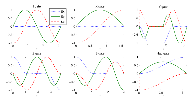
Figure 6: Time-evolution of Bloch vector components ${\bf s}=(x,y,z)$ for various elementary gates using local geometric control with time in units of $\frac{\pi}{2}\Omega^{-1}$, where $\Omega$ is the Rabi frequency of the fixed global field.

In summary, we can in principle implement quantum logic gates on encoded qubits using simple control pulse sequences based on geometric control ideas in both the local and global control setting. However, the simple schemes have serious shortcomings. Frequency-selective global control schemes, for instance, requires comparatively long pulses to minimize off-resonant excitation. In the local control setting it is difficult to implement different gates concurrently on different qubits due to variable gate operation times. Both schemes also assume non-interacting physical qubits, and tend to perform poorly in the presence of fixed couplings due the creation of entanglement between qubits. Also, some essential gates such as the $T$-gate cannot be implemented transversally at all. This raises the question if we can overcome such problems using optimal control, which we will consider in the next sections.

4 Optimal Control

The problem of finding the control pulses that produce the desired quantum gates can be treated as an optimization problem. The procedure in general involves choosing a measure of the gate fidelity to be maximized, suitably parameterizing the control fields and finding a solution to the resulting optimization problem. If the evolution of the system is given by a unitary operator $U(t)$ satisfying the Schroedinger equation

$$\dot{U}(t,t_{0})=-\frac{i}{\hbar}\left[H_{0}+\sum_{m=1}^{M}u_{m}(t)H_{m}\right]U(t,t_{0}),$$ (17)

where $H_{0}$ is a drift Hamiltonian and $H_{m}$, $m=1,\ldots M<\infty$, are control Hamiltonians, the task is to find a control ${\bf u}(t)$ that maximizes the gate fidelity

$$\mathcal{F}_{W}[U(t_{F},t_{0})]=\frac{2}{N}\Re\Tr[W^{\dagger}U(t_{F},t_{0})]$$ (18)

or similar figure of merit for some fixed target time $t_{F}$ .

To derive an iterative procedure for finding optimal controls, note that changing a given control ${\bf u}$ by some amount $\Delta{\bf u}$ changes the corresponding propagator (see A)

$$\Delta U_{\mathbf{u}}(t,t_{0}) \equiv U_{{\bf u+\Delta u}}(t,t_{0})-U_{{\bf u}}(t,t_{0})$$ (19)

$$= -\frac{i}{\hbar}\int_{t_{0}}^{t}\sum_{m}\Delta u_{m}(\tau)U_{{\bf u}}(t,\tau)H_{m}U_{{\bf u}+{\bf\Delta u}}(\tau,t_{0})\,d\tau.$$

The corresponding change in the fidelity is

$$\Delta\mathcal{F}(t_{F}) = \mathcal{F}_{\mathbf{u+\Delta u}}(t_{F})-\mathcal{F}_{\mathbf{u}}(t_{F})$$

$$= \frac{2}{N}\Re\Tr[W^{{\dagger}}(U_{{\bf u+\Delta u}}(t_{F},t_{0})-U_{{\bf u}}(t_{F},t_{0}))]$$

$$= \frac{2}{N\hbar}\sum_{m}\int_{t_{0}}^{t_{F}}\!\!\!\!\Delta u_{m}(\tau)\Im\Tr[W^{{\dagger}}U_{{\bf u}}(t_{F},\tau)H_{m}U_{{\bf u+\Delta u}}(\tau,t_{0})]\,d\tau.$$

This shows that setting

$$\Delta u_{m}(t)=\epsilon_{m}(t)\Im\Tr[W^{{\dagger}}U_{{\bf u}}(t_{F},t)H_{m}U_{{\bf u+\Delta u}}(t,t_{0})]$$ (21)

with $\epsilon_{m}(t)>0$ for all $t$ will increase the fidelity at the target time $t_{F}$. Thus, a basic algorithm for maximizing $\mathcal{F}$ is to start with some initial guess ${\bf u}_{0}(t)$ and solve the Schroedinger equation iteratively while updating the control according to the rule

$${\bf u}^{(n+1)}={\bf u}^{(n)}+\Delta{\bf u}^{(n)},$$ (22)

with $\Delta{\bf u}^{(n)}$ as in (21). Note that this is an implicit update rule as the RHS of (21) depends on $\Delta{\bf u}(t)$, and the search space is infinite dimensional, consisting of functions on defined on an interval of the real line.

To derive useful practical algorithms the controls $u_{m}(t)$ need to be discretized, and a simplified explicit update rule is desirable. The simplest and most common approach to discretization is to approximate the continuous fields by piecewise constant functions, i.e., we divide the total time $t_{F}$ into $K$ steps, usually, though not necessarily, of equal duration $\Delta t=t_{F}/K$, and take the control amplitudes to be constant during each interval $I_{k}=[t_{k-1},t_{k})$. We then have

$$\mathcal{F}_{W}[U(t_{F})]=\frac{2}{N}\Re\Tr\left[W^{\dagger}U_{{\bf u}}^{(K)}U_{{\bf u}}^{(K-1)}\cdots U_{{\bf u}}^{(2)}U_{{\bf u}}^{(1)}\right],$$ (23)

where the step propagator for the $k$th step is given by

$$U_{{\bf u}}^{(k)}=\exp\left[-\frac{i}{\hbar}\Delta t\left(H_{0}+\sum_{m=1}^{M}u_{mk}H_{m}\right)\right]$$ (24)

and $u_{mk}$ is the amplitude of the $m$th control field during the $k$th step. Furthermore, if we change the control field by $\Delta u_{m}(t)=\Delta u_{mk}$ for $t\in I_{k}$ then the change in the fidelity at the target time $t_{F}$ is (see B)

$$\Delta\mathcal{F}(t_{F})=\frac{2}{N\hbar}\sum_{m}\Delta u_{mk}\Im\Tr\left[W^{\dagger}U_{{\bf u}}^{(K)}\cdots U_{{\bf u}}^{(k+1)}\Delta U_{m}^{(k)}U_{{\bf u}+\Delta{\bf u}}^{(k-1)}\ldots U_{{\bf u}+\Delta{\bf u}}^{(1)}\right]$$ (25)

with $U_{{\bf u}}^{(k)}$ and $U_{{\bf u}+\Delta{\bf u}}^{(k)}$ as defined in (24) and

$$\Delta U_{m}^{(k)}=\int_{t_{k-1}}^{t_{k}}\!\!\!U_{{\bf u}}(t_{k},\tau)H_{m}U_{{\bf u+\Delta u}}(\tau,t_{k-1})]\,d\tau.$$ (26)

This shows that the fidelity will increase at time $t_{F}$ if we change the field amplitude $u_{mk}$ in the time interval $I_{k}$ by

$$\Delta u_{mk}=\epsilon_{mk}\Im\Tr\left[W^{\dagger}U_{{\bf u}}^{(K)}\cdots U_{{\bf u}}^{(k+1)}\Delta U^{(k)}(t)U_{{\bf u}+\Delta{\bf u}}^{(k-1)}\ldots U_{{\bf u}+\Delta{\bf u}}^{(1)}\right]$$

for $\epsilon_{mk}>0$. This is still an implicit update rule as $\Delta U^{(k)}$ on the RHS depends $\Delta u_{mk}$. However, when $\Delta t=t_{k}-t_{k-1}$ and $\Delta u_{mk}$ are sufficiently small then we can approximate $\Delta U_{m}^{(k)}$, e.g., setting $\Delta U_{m}^{(k)}\approx U_{{\bf u}}^{(k)}H_{m}$, which yields the familiar explicit update rule

$$\Delta u_{mk}=\epsilon_{mk}\Im\Tr\left[W^{\dagger}U_{{\bf u}}^{(K)}\cdots U_{{\bf u}}^{(k)}H_{m}U_{{\bf u}+\Delta{\bf u}}^{(k-1)}\ldots U_{{\bf u}+\Delta{\bf u}}^{(1)}\right].$$ (27)

In practice we can now solve the optimization problem by starting with an initial guess for the controls ${\bf u}_{m}^{(0)}$, calculating $U^{(0)}(t_{F})$ and then integrating alternatingly backwards and forwards while updating the controls in each time step according to the explicit update rule (27) until no further improvement in the fidelity is possible. Ignoring errors to due numerics (e.g. limited precision floating point arithmetic, etc), if the algorithm is implemented strictly as presented and the $\epsilon_{mk}$ are chosen in each time step and iteration such that the value of the fidelity at the final time does not decrease, then convergence is guaranteed as the fidelity is nondecreasing and bounded above. However, we cannot guarantee that the fidelity will converge to the global maximum, especially when there are constraints on the field amplitudes or time resolution $\Delta t$ of the fields. The algorithm will stop when it is no longer possible to change $u_{mk}$ for any $m$ or $k$ such as to increase the final fidelity.

The update rule (27) is similar to the update rule of the familiar GRAPE algorithm [14], but in the GRAPE algorithm the update is global, i.e., the field amplitudes $u_{mk}$ for all times $t_{k}$ are updated concurrently in each iteration step based on the propagators $U^{(k)}_{{\bf u}}$ using the fields from the previous iteration step, which is equivalent to setting

$$\Delta u_{mk}=\epsilon_{m}\Im\Tr\left[W^{\dagger}U_{{\bf u}}^{(K)}\cdots U_{{\bf u}}^{(k)}H_{m}U_{{\bf u}}^{(k-1)}\ldots U_{{\bf u}}^{(1)}\right]$$ (28)

for all $m$ and $k$. This global update has certain advantages such as easy parallelizability, but it requires the field changes in each step to be small to maintain the validity of the approximations involved and ensure an overall increase in the fidelity. The parameter $\epsilon_{m}$ is critical in this regard and must be chosen carefully to ensure monotonic convergence. One way this can be achieved is by choosing $\epsilon_{m}$ to be very small (steepest decent) but this comes at the expense of very slow convergence. In practice one would therefore usually employ step-size control in the form of linesearch, quasi-Newton methods or conjugate gradients to accelerate convergence.

Despite the similarities in the update rules, the sequential local update method is quite different. With sequential local update the fidelity increases in every time step, not just for every iteration, and we can make much larger changes to the field(s) in each step, with the magnitude of the allowed changes limited mainly by explicit constraints on the field amplitudes and the approximations involved in transforming the implicit update rule to an explicit one, which could be avoided or improved, and discretization errors. The sequential local update rule also allows us to easily enforce certain local constraints. For example, a constraint on the field amplitudes of the form $|u_{m}(t)|<C$ can be trivially incorporated as we simply have to choose $\epsilon_{mk}$ in each time step $k$ so that $|u_{mk}+\Delta u_{mk}|\leq C$. Assuming the initial controls is choosen such that the constraints are satisfied, $|u_{mk}|\leq C$, this is always possible, if necessary by setting $\epsilon_{mn}=0$ for this time step. In this case there will, of course, be no increase of the final fidelity during this time step but we will generally be able to continue to increase the fidelity in the next time steps, although such an amplitude constraint may eventually prevent us from increasing the fidelity further for all time steps, in which case we could be left with a solution for which final fidelity is less than its optimum value. Of course, amplitude constraints can also be incorporated in global update schemes, albeit not quite as trivially. Another perhaps more interesting feature of the sequential update method is that it enables us use variable time steps to increase the fidelity further should a given time resolution of the fields prove insufficient to achieve high-enough fidelities.

The sequential local update method is similar to a class of methods often referred to as the Krotov method, based on work by Krotov [15, 16], adapted to quantum systems by Tannor et al [17], although our formulation is for unitary operators rather than quantum states and there is no penalty on field energy.

5 Optimal Control Implementation of Encoded Logic Gates

We now apply optimal control algorithm described in the previous section to the problem of implementing fault-tolerant logic gates for the five-qubit stabilizer code. In particular, we wish to implement a full set of elementary logic gates in a fixed amount of time for systems subject to both inhomogeneity and interactions between adjacent qubits. For the global control system we choose the total Hamiltonian

$$H^{(\rm g)}[{\bf u}(t)]=-\frac{1}{2}\sum_{n=1}^{5}\omega_{n}\sigma_{z}^{(n)}+J\sum_{n=1}^{4}\sigma_{z}^{(n)}\sigma_{z}^{(n+1)}+u_{1}(t)\sum_{n=1}^{5}\sigma_{x}^{(n)}+u_{2}(t)\sum_{n=1}^{5}\sigma_{y}^{(n)}\quad$$ (29)

with $\omega_{n}\in\{6,8,10,12,14\}$, and the aim is to optimize the two fields $u_{1}(t)$ and $u_{2}(t)$, which roughly correspond to the $x$ and $y$ components of an external electromagnetic field, to implement the desired encoded logic gates. For the local control case we choose the Hamiltonian

$$H^{(\rm l)}[{\bf u}(t)]=\Omega\sum_{n}\sigma_{x}^{(n)}+J\sum_{n=1}^{4}\sigma_{z}^{(n)}\sigma_{z}^{(n+1)}+\sum_{n}u_{n}(t)\sigma_{z}^{(n)}$$ (30)

where $u_{n}(t)$ for $n=1,2,3,4,5$ are controls that induces local detunings and $\Omega=10$ is the Rabi frequency of the fixed external coupling field. Here we have chosen units such that $\hbar=1$.

In order to find the optimal solutions using the algorithm outlined above we must choose the number of time-steps $K$ and the total time $t_{F}$ and a suitable initial control ${\bf u}^{(0)}$. To ensure that the gates are fast and do not require controls with extremely high time resolution, we aspire to find solutions for $t_{F}$ and $K$ small. Unfortunately, there are no simple rules for choosing $t_{F}$ and $K$. With some experimentation we were able to find controls that achieved gate fidelities of approximately $99.99$ % for the global control example with $J=1$ for $t_{F}=125$ with $K=1250$ time steps. For the local control example $t_{F}=30$ and $K=300$ proved sufficient. The gate operation times achieved using optimal controls in the global control setting, although much longer than for the local controls, are still favorable compared to frequency-selective geometric control pulses, for which even the $X$-gate required approximately $500$ time units for $J=0$ and the method failed for $J$ greater than $10^{-4}$. Although the local gates for $\Omega=10$ are much slower than what is theoretically possible using local geometric control in the absence of coupling, the optimal controls have the distinct advantage that they enable us to implement all gates in a fixed amount of time and deal with non-zero $J$-couplings. Also, the implementation of the $T$-gate, which can not be implemented transversally, presents no greater challenge for optimal control than any of the other gates. In fact, the simulations suggest that the most difficult gate to implement in the global control setting is the $Y$-gate. In the local control setting there appeared to be little difference in the difficulty of implementing different gates.

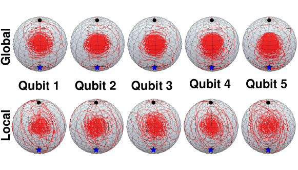
Figure 7: Evolution of physical qubits initialized in the state $\ket{00000}$ subject to the optimal controls required to implement the $X$-gate.

For comparison with the geometric control results, Fig. 7 shows the trajectories of the physical qubits subject to the optimal controls for the logic $X$-gate. Again, the qubits were assumed to be initialized in the product state $\ket{00000}$. This is not a logic state but allows us to easily check visually that the gate effects the desired simultaneous bit flip on all physical qubits even in the presence of significant inter-qubit couplings ($J=1$). The single-qubit trajectories start out at the surface (north pole) of the Bloch sphere, corresponding to the product state $\ket{00000}$. They descend inside the Bloch ball as the qubits then become entangled, and the individual qubits follow different paths, but at the final time the trajectories of all physical qubits converge to the south pole of the Bloch sphere, as desired.

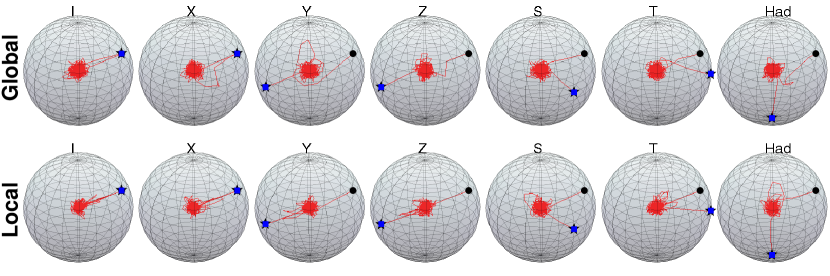
Figure 8: Controlled evolution of the initial state $\ket{\Psi(0)}=(\ket{0_{L}}+\ket{1_{L}})/\sqrt{2}$ projected onto the 2D subspace spanned by $\ket{0_{L}}$ and $\ket{1_{L}}$ for different logic gates for optimal control examples with global and local control.

To get an idea of how the optimal controls perform for the other gates beyond the gate fidelity, Fig. 8 shows the projection of the controlled evolution onto the two-dimensional subspace of the Hilbert space spanned by the logic states $\ket{0_{L}}$ and $\ket{1_{L}}$ for the initial state $\ket{\Psi(0)}=\frac{1}{\sqrt{2}}(\ket{0_{L}}+\ket{1_{L}})$. The Bloch vector was defined to be

$$s_{x}(t) = 2\Re\left[\langle 0_{L}\mid\Psi(t)\rangle\langle\Psi(t)\mid 1_{L}\rangle\right]$$ (31)

$$s_{y}(t) = -2\Im\left[\langle 0_{L}\mid\Psi(t)\rangle\langle\Psi(t)\mid 1_{L}\rangle\right]$$ (32)

$$s_{z}(t) = |\langle 1_{L}\mid\Psi(t)\rangle|^{2}-|\langle 0_{L}\mid\Psi(t)\rangle|^{2},$$ (33)

where $\ket{\Psi(t)}=U(t)\ket{\Psi(0)}$ and $U(t)$ is the full $32\times 32$ unitary operator describing the evolution of the system under the given optimal control. The plots show that the evolution of the system is very complicated. Although the initial state is in the 2D subspace spanned by the logic states $\ket{0_{L}}$ and $\ket{1_{L}}$, the fact that the trajectories (red) are concentrated in the interior of the Bloch ball indicates that the system spends most of the time outside the two-dimensional logic subspace, but returns (mostly) to this subspace near the final time. Although the gate fidelities as defined in (18) are about $99.99$ %, there are small but noticeable differences between the actual final states ($\bigstar$) and the final states (blue squares) for an ideal gate. This is due to the fact that the normalized gate fidelity for high-dimensional gates is not a very strict measure as

$$\|W-U(t_{F})\|_{2} =\sqrt{\Tr[(W-U)^{\dagger}(W-U)]}$$

$$=\sqrt{2N[1-\mathcal{F}_{W}(U)]},$$

with $\mathcal{F}_{W}(U)$ as defined in Eq. (18), i.e., the distance between the operators with respect to the Hilbert-Schmidt norm is significantly larger than the gate error defined in terms of the fidelity $1-\mathcal{F}_{W}[U(t_{F})]$. For $N=32$ a gate fidelity of $>99.99$ % allows a Hilbert-Schmidt distance between the operators up to $0.08$. The distance between the operators with respect to the operator norm $\|X\|$ (given by the largest singular value of $X$) is usually smaller than the Hilbert Schmidt distance but still significantly larger than the fidelity error. A summary of different gate error measures for all gates is given in Table 3.

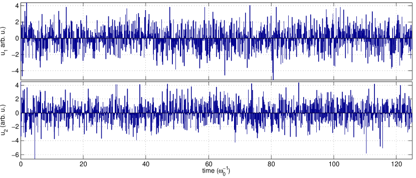
Figure 9: Example of optimal control solution to implement the non-transversal $T$-gate for the five qubit stabilizer code using two independent global fields for system (29).

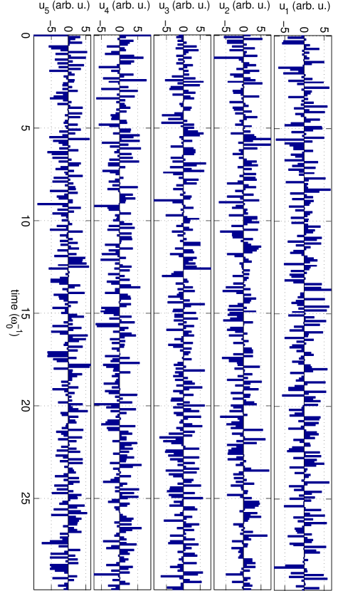
Figure 10: Example of optimal control solution to implement the non-transversal $T$-gate for the five qubit stabilizer code using five independent local detuning fields for system (30).

Examples of the actual control fields obtained in both the local and global control setting are shown in Figures 9 and 10 for the $T$-gate. The control fields appear complicated, especially in the global control case. The local control fields appear to be better behaved but this is is in part due to the scaling of the time axis — the global control pulses are much longer and thus appear much more compressed when scaled to fit the width of the text. Nonetheless the controls are complicated and have a relatively high bandwidth. To some extent this is unsurprising considering the complexity of the system, control goals, and constraints imposed on the controls in terms of pulse lengths and time resolutions. However, there are many possible controls that result in the same gate, corresponding to alternative trajectories in $SU(N)$ connecting the identity and the target gate. A limited number of numerical experiments performed with different choices for the initial fields suggest that these lead to different solutions for the controls, but generally the solutions appear to have similar complexities. However, it may be possible to exploit the non-uniqueness of the solutions to find better solutions, either by changing the parameterization of the fields or imposing carefully chosen additional penalty terms, which we will consider in future work.

		I	X	Y	Z	S	T	Had
global	$\mathcal{F}_{W}(U)$	0.9999	0.9999	0.9996	0.9999	0.9999	0.9999	0.9999
	$\|W-U\|$	0.0267	0.0268	0.0573	0.0259	0.0255	0.0261	0.0266
	$\|W-U\|_{2}$	0.0800	0.0800	0.1644	0.0800	0.0800	0.0800	0.0800
	$\|W-U\|_{\max}$	0.0061	0.0069	0.0163	0.0074	0.0064	0.0071	0.0065
local	$\mathcal{F}_{W}(U)$	0.9999	0.9999	0.9999	0.9999	0.9999	0.9999	0.9999
	$\|W-U\|$	0.0268	0.0266	0.0266	0.0253	0.0252	0.0250	0.0263
	$\|W-U\|_{2}$	0.0799	0.0798	0.0799	0.0798	0.0798	0.0798	0.0799
	$\|W-U\|_{\max}$	0.0056	0.0069	0.0069	0.0058	0.0069	0.0068	0.0066

Table 3: Different performance measures for the gates implemented using optimal control: Fidelity, operator distance $\|W-U\|$ (largest singular value of $W-U$), Hilbert-Schmidt distance $\|W-U\|_{2}=\sqrt{\Tr[(W-U)^{\dagger}(W-U)]}$, and maximum distance between matrix elements $\|W-U\|_{\max}=\max_{m,n}|W_{mn}-U_{mn}|$, where $U=U(t_{F})$ and $W$ is the target gate.

The presence of fixed couplings between the qubits, which was highly detrimental for the geometric control schemes, does not appear to be a problem in the optimal control case, and indeed some of our simulations suggested that larger $J$-couplings may in fact make it easier to find optimal control solutions. This apparently counter-intuitive behavior prompted us to consider the effect of varying the interqubit coupling strength $J$ and the detunings $\Delta\omega$. We can get an estimate of the difficulty of finding solutions by setting $t_{F}$ and $K$ to constant values and comparing the number of iterations required to archive $99.99$% fidelity for various values of $J$ and $\Delta\omega$. A small number of iterations generally implies that it is easy to find a solution and that solutions may exist for significantly shorter times $t_{F}$. To reduce the computational overhead, we considered the same model systems but with only three instead of five qubits, and taking as target gates the standard gates for the three-qubit bit-flip code with code words $\ket{0_{L}}=\ket{000}$ and $\ket{1_{L}}=\ket{111}$. For this system the run time of the optimization routine reduces from several hours for the five qubit code to a few minutes on a single 3GHz CPU. It proved easy to find solutions for the system subject to global control with $J=1$ for $t_{F}=10$ and $K=80$, so we selected these values as defaults. Fig. 11(a) shows the number of iterations for different values of $J$. Although the number of iterations required for convergence maybe an oversimplified measure of the complexity, the data indeed suggests that increasing $J$ makes it easier for the algorithm to find solutions, suggesting that optimal control allows us to exploit couplings that are usually considered undesirable to speed up gate operations, especially in the global control setting. The effect of changing $\Delta\omega$ is more subtle. If $\Delta\omega$ is very small then the selectivity of the pulses is very weak and the algorithms struggles to find solutions unless $t_{F}$ is increased. If $\Delta\omega$ is very large then it is also hard to find the solutions, partly because the system can not use off-resonant excitations as much, but more likely because the bandwidth of the fields available may not be sufficient to cover the required frequency range.

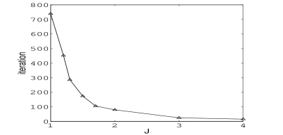
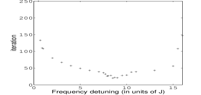
Figure 11: Number of iterations required to find solutions with $\mathcal{F}_{W}(U)\geq 0.9999$ for (a) $t_{F}=10$, $M=80$ and $\Delta\omega=2$; (b) $t_{F}=10$, $M=80$ and $J=2$.

6 Conclusion

We have considered the problem of implementing quantum logic gates acting on encoded qubits, As a particular example, the five-qubit stabilizer code was considered. Despite the complicated encoding, most elementary logic gates can in principle be implemented fault-tolerantly by applying the same local gates to all physical qubits. Thus, it is usually argued that the implementation of logic gates on encoded qubits can be reduced to the implementation of single and two-qubit gates on physical qubits, and that the latter can in principle be implemented using simple pulse sequences based geometric control ideas. However, there are several problems with this. Not all gates can be implemented transversally. For the five-qubit code, for instance, it is not possible to implement a $T$-gate this way, which is an essential gate for universal quantum computation. Moreover, for realistic physical systems inhomogeneity and often uncontrollable interactions between nearby physical qubits pose significant problems, rendering simple gate implementation schemes based transversal application of single-qubit geometric pulse sequences ineffective.

Using an optimal control approach we can in principle overcome these problems and find effective control pulse sequences to implement encoded logic gates even for imperfect systems subject to limited control, e.g., if we are unable to selectively address individual qubits, or switch off unwanted interactions between qubits. Perhaps even more importantly, the implementation of gates that are difficult to implement using conventional techniques such as the $T$-gate for the five-qubit stabilizer code, appears to present no greater challenge for optimal control than the implementation of any other gate. A potential drawback at present is the complexity of the optimal control solutions. However, the optimal control solutions are not unique, and the solutions found here should therefore be regarded more as a demonstration of principle, i.e., that is is possible to find solutions to the optimal control problem. Simpler solutions are likely to exist at least for certain problems, and future work exploring whether such solutions can be found by considering different field parameterizations or imposing suitable penalty terms that steer the algorithm away from complicated fields towards simpler solutions (if they exist) could be fruitful.

References

Appendix A Derivation of Eq. (19)

Letting for convenience

$$H_{0}^{\prime}(t) = H_{0}+\sum_{m}u_{m}(t)H_{m}$$

$$H_{1}^{\prime}(t) = \sum_{m}\Delta u_{m}(t)H_{m}.$$

we can rewrite the Schrodinger equation for $U_{{\bf u}}(t,t_{0})$ and $U_{{\bf u}+{\bf\Delta u}}(t,t_{0})$ as

$$\dot{U}_{{\bf u}}(t,t_{0}) = -\frac{i}{\hbar}H_{0}^{\prime}(t)U_{{\bf u}}(t,t_{0}),$$

$$\dot{U}_{{\bf u}+{\bf\Delta u}}(t,t_{0}) = -\frac{i}{\hbar}[H_{0}^{\prime}(t)+H_{1}^{\prime}(t)]U_{{\bf u}+{\bf\Delta u}}(t,t_{0}).$$

Inserting an interaction picture decomposition

$$U_{{\bf u}+{\bf\Delta u}}(t,t_{0})=U_{{\bf u}}(t,t_{0})U_{I}(t,t_{0})$$ (35)

into the Schrodinger equation we obtain using the product rule

$$\dot{U}_{I}(t,t_{0})=-\frac{i}{\hbar}[U_{{\bf u}}(t,t_{0})^{\dagger}H_{1}^{\prime}(t)U_{{\bf u}}(t,t_{0})]U_{I}(t,t_{0}).$$

Rewriting this differential equation in integral form gives

$$U_{I}(t,t_{0})=\mathbb{I}-\frac{i}{\hbar}\int_{t_{0}}^{t}[U_{{\bf u}}(\tau,t_{0})^{\dagger}H_{1}^{\prime}(\tau)U_{{\bf u}}(\tau,t_{0})]U_{I}(\tau,t_{0})\,d\tau$$

Multiplying both sides by $U_{{\bf u}}(t,t_{0})$ and noting that $U_{{\bf u}}(t,t_{0})$ does not depend on $\tau$ and thus can be moved inside the integral now yields

$$U_{{\bf u}+{\bf\Delta u}}(t,t_{0}) = U_{{\bf u}}(t,t_{0})-\frac{i}{\hbar}\int_{t_{0}}^{t}U_{{\bf u}}(t,t_{0})U_{{\bf u}}(\tau,t_{0})^{\dagger}H_{1}^{\prime}(\tau)U_{{\bf u}}(\tau,t_{0})U_{I}(\tau,t_{0})\,d\tau$$

$$= U_{{\bf u}}(t,t_{0})-\frac{i}{\hbar}\int_{t_{0}}^{t}U_{{\bf u}}(t,\tau)H_{1}^{\prime}(\tau)U_{{\bf u}+{\bf\Delta u}}(\tau,t_{0})\,d\tau$$

$$= U_{{\bf u}}(t,t_{0})-\frac{i}{\hbar}\int_{t_{0}}^{t}\sum_{m}\Delta u_{m}(t)U_{{\bf u}}(t,\tau)H_{m}U_{{\bf u}+{\bf\Delta u}}(\tau,t_{0})\,d\tau$$

where we have used $U_{{\bf u}}(t,t_{0})U_{{\bf u}}(\tau,t_{0})^{\dagger}=U_{{\bf u}}(t,\tau)$ we as well as Eq. (35) and the definition of $H_{1}^{\prime}(t)$.

Appendix B Derivation of Eq. (25)

If $\Delta u_{m}(t)=0$ except for $t\in I_{k}=[t_{k-1},t_{k}]$ then we have

$$\Delta\mathcal{F}(t_{F}) = \frac{2}{N\hbar}\sum_{m}\int_{t_{0}}^{t_{F}}\!\!\!\Delta u_{m}(\tau)\Im\Tr[W^{{\dagger}}U_{{\bf u}}(t_{F},\tau)H_{m}U_{{\bf u+\Delta u}}(\tau,t_{0})]\,d\tau$$

$$= \frac{2}{N\hbar}\sum_{m}\int_{t_{k-1}}^{t_{k}}\!\!\!\Delta u_{m}(\tau)\Im\Tr[W^{{\dagger}}U_{{\bf u}}(t_{F},\tau)H_{m}U_{{\bf u+\Delta u}}(\tau,t_{0})]\,d\tau$$

Furthermore, we have $U_{{\bf u}}(t_{F},\tau)=U_{{\bf u}}(t_{F},t_{k})U_{{\bf u}}(t_{k},\tau)$ as well as $U_{{\bf u+\Delta u}}(\tau,t_{0})=U_{{\bf u+\Delta u}}(\tau,t_{k-1})U_{{\bf u+\Delta u}}(t_{k-1},t_{0})$ and because $U_{{\bf u}}(t_{F},t_{k})$ and $U_{{\bf u+\Delta u}}(t_{k-1},t_{0})$ are outside of the domain of integration we can re-write the expression for $\Delta\mathcal{F}(t_{F})$ as

$$\Delta\mathcal{F}(t_{F})=\frac{2}{N\hbar}\sum_{m}\Delta u_{m}(\tau)\Im\Tr\left[W^{{\dagger}}U_{{\bf u}}(t_{F},t_{k})\Delta U_{m}^{(k)}U_{{\bf u+\Delta u}}(t_{k},t_{0})\right]$$

with $\Delta U_{m}^{(k)}$ as in (26). Finally noting that

$$U_{{\bf u}}(t_{F},t_{k}) = U_{{\bf u}}^{(K)}\cdots U_{{\bf u}}^{(k+1)}$$

$$U_{{\bf u+\Delta u}}(t_{k},t_{0}) = U_{{\bf u}+\Delta{\bf u}}^{(k-1)}\ldots U_{{\bf u}+\Delta{\bf u}}^{(1)}$$

with $U_{{\bf u}}^{(k)}$ and $U_{{\bf u}+\Delta{\bf u}}^{(k)}$ as defined in (24) gives

$$\Delta\mathcal{F}(t_{F})=\frac{2}{N\hbar}\sum_{m}\Delta u_{mk}\Im\Tr\left[W^{\dagger}U_{{\bf u}}^{(K)}\cdots U_{{\bf u}}^{(k+1)}\Delta U_{m}^{(k)}U_{{\bf u}+\Delta{\bf u}}^{(k-1)}\ldots U_{{\bf u}+\Delta{\bf u}}^{(1)}\right]$$

References

- [1] L. M. K. Vandersypen, I. L.Chuang, Rev. Mod. Phys. 76, 1037 (2004)
- [2] A. M. Stephens et al. Phys. Rev. A 78, 032318 (2008).
- [3] D. Leibfried et al. Hyperfine Interactions 174, 1 (2007).
- [4] C. Ospelkaus et al. Phys. Rev. Lett 101, (2008).
- [5] F. Perez-Martinez et al. Appl. Phys. Lett. 91, 032102 (2007).
- [6] L. Robledo et al. Science 320, 772 (2008).
- [7] N. Khaneja and S. Glaser, Chem. Phys. 267, 11–23 (2001)
- [8] T. Schulte-Herbruggen, A. Sporl, N. Khaneja, S. Glaser, Phys. Rev. A 72(4), 042331 (2005)
- [9] S. Schirmer, J. Mod. Opt. 56, 831 (2009).
- [10] M. A. Nielsen and I. L. Chuang, Quantum Computation and Quantum Information (Cambridge University Press, 2000), Chapter 10 on Error Correction and Fault-tolerant Computation.
- [11] C. D. Hill et al., Phys. Rev. B 72(4), 045350 (2005)
- [12] G. Kandasamy, C. J. Wellard, L.C.L. Hollenberg, Nanotechnology 17, 4572 (2006)
- [13] S. G. Schirmer, G. Kandasamy, L. C. L. Hollenberg, AIP Conf. Proc. 963, Part B, Vol. 2 (2007)
- [14] N. Khaneja, T. Reiss, C. Kehlet, T. S-Herbruggen, S. Glaser, J. Mag. Res. 172, 296-305 (2005)
- [15] V. F. Krotov, I. N. Feldman, Izv. Akad. Nauk SSSR, Tekh. Kibern. 2, 160-168 (1983)
- [16] A. I. Konnov and V. F. Krotov, Automation and Remote Control 60, 1427 (1999)
- [17] D.J. Tannor, V. Kazakov and V. Orlov, In: Time Dependent Quantum Molecular Dynamics, J. Broeckhove and L. Lathouwers, eds., 347-360 (Plenum, 1992).