Holographic Dark Energy Model with Hubble Horizon as an IR Cut-off

Abstract

The main task of this paper is to realize a cosmic observational compatible universe in the framework of holographic dark energy model when the Hubble horizon $H$ is taken as the role of an IR cut-off. When the model parameter $c$ of a time variable cosmological constant (CC) $\Lambda(t)=3c^{2}H^{2}(t)$ becomes time or scale dependent, an extra term enters in the effective equation of sate (EoS) of the vacuum energy $w^{eff}_{\Lambda}=-c^{2}-d\ln c^{2}/3d\ln a$. This extra term can make the effective EoS of time variable CC cross the cosmological boundary and be phantom-like at present. For the lack of a first principle and fundamental physics theory to obtain the form $c^{2}$, we give a simple parameterized form of $c^{2}$ as an example. Then the model is confronted by the cosmic observations including SN Ia, BAO and CMB shift parameter $R$. The result shows that the model is consistent with cosmic observations.

ITP-DUT/2009-07

I Introduction

The observation of the Supernovae of type Ia ref:Riess98 ; ref:Perlmuter99 provides the evidence that the universe is undergoing accelerated expansion at present. Combining the observations from Cosmic Background Radiation ref:Spergel03 ; ref:Spergel06 and SDSS ref:Tegmark1 ; ref:Tegmark2 , one concludes that the universe at present is dominated by $70\%$ exotic component, dubbed dark energy, which has negative pressure and pushes the universe to accelerated expansion. Of course, a natural explanation to the accelerated expansion is due to a positive tiny cosmological constant. Though, it suffers the so-called fine tuning and cosmic coincidence problems. However, in $2\sigma$ confidence level, it fits the observations very well ref:Komatsu . If the cosmological constant is not a real constant but is time variable, the fine tuning and cosmic coincidence problems can be removed. In fact, this possibility was considered in the past years.

In particular, the dynamic vacuum energy density based on holographic principle was investigated extensively ref:holo1 ; ref:holo2 . According to the holographic principle, the number of degrees of freedom in a bounded system should be finite and has relations with the area of its boundary. By applying the principle to cosmology, one can obtain the upper bound of the entropy contained in the universe. For a system with size $L$ and UV cut-off $\Lambda$ without decaying into a black hole, it is required that the total energy in a region of size $L$ should not exceed the mass of a black hole of the same size, thus $L^{3}\rho_{\Lambda}\leq LM^{2}_{P}$. The largest $L$ allowed is the one saturating this inequality, thus $\rho_{\Lambda}=3c^{2}M^{2}_{P}L^{-2}$, where $c$ is a numerical constant and $M_{P}$ is the reduced Planck Mass $M^{-2}_{P}=8\pi G$. It just means a duality between UV cut-off and IR cut-off. The UV cut-off is related to the vacuum energy, and IR cut-off is related to the large scale of the universe, for example Hubble horizon, future event horizon or particle horizon which were discussed by ref:holo1 ; ref:holo2 ; ref:Horvat1 ; ref:Horvat2 . The holographic dark energy in Brans-Dicke theory was also studied in Ref. ref:BransDicke ; ref:BDH1 ; ref:BDH2 ; ref:BDH3 ; ref:BDH4 ; ref:BDH5 . In the standard and Brans-Dicke holographic dark energy models when the Hubble horizon is taken as the role of IR cut-off, non-accelerated expansion universe can be achieved ref:holo1 ; ref:holo2 ; ref:BransDicke . However, the Hubble horizon is the most natural cosmological length scale, how to realize an accelerated expansion by taking it as an IR cut-off will be interesting.

Furthermore, the holographic cosmological constant were discussed in ref:Horvat1 ; ref:Horvat2 ; ref:Feng , where a time variable cosmological constant comes from the holographic principle. Inspired by the observation of the relation between cosmological length or time scale with any nonzero value of the cosmological constant $r_{\Lambda}=t_{\Lambda}=\sqrt{3/|\Lambda|}$, horizon cosmological constants were discussed in Xu:TVCC . In these two cases, an accelerated expansion universe could be obtained at present, precisely speaking a scaling solution was obtained, when the Hubble horizon was taken as the role of an IR cut-off. But unfortunately, non-transition from decelerated expansion to accelerated expansion can be realized in this scenario. This observation motivates us to consider the possibility of realizing accelerated expansion by mini modification of holographic or horizon cosmological constant model. This will be the main task of this work.

This paper is structured as follows. In Section II, we give a brief review of time variable cosmological constant. In Section III, Hubble horizon as an IR cut-off will be explored when $c$ is fixed constant and time or scale dependent respectively. In this section, cosmic observational constraint is also implemented. Where the cosmic observations and constraint methods are put in the Appendix A. Conclusions are set in Section IV.

II Time Variable Cosmological Constant

The Einstein equation with a cosmological constant is written as

$$R_{\mu\nu}-\frac{1}{2}Rg_{\mu\nu}+\Lambda g_{\mu\nu}=8\pi GT_{\mu\nu},$$ (1)

where $T_{\mu\nu}$ is the energy-momentum tensor of ordinary matter and radiation. From the Bianchi identity, one has the conservation of the energy-momentum tensor $\nabla^{\mu}T_{\mu\nu}=0$, it follows necessarily that $\Lambda$ is a constant. To have a time variable cosmological constant $\Lambda=\Lambda(t)$, one can move the cosmological constant to the right hand side of Eq. (1) and take $\tilde{T}_{\mu\nu}=T_{\mu\nu}-\frac{\Lambda(t)}{8\pi G}g_{\mu\nu}$ as the total energy-momentum tenor. Once again to preserve the Bianchi identity or local energy-momentum conservation law, $\nabla^{\mu}\tilde{T}_{\mu\nu}=0$, one has, in a spatially flat FRW universe,

$$\dot{\rho}_{\Lambda}+\dot{\rho}_{m}+3H\left(1+w_{m}\right)\rho_{m}=0,$$ (2)

where $\rho_{\Lambda}=M^{2}_{P}\Lambda(t)$ is the energy density of time variable cosmological constant and its equation of state is $w_{\Lambda}=-1$, and $w_{m}$ is the equation of state of ordinary matter, for dark matter $w_{m}=0$. It is natural to consider interactions between variable cosmological constant and dark matter ref:Horvat2 , as seen from Eq. (2). After introducing an interaction term $Q$, one has

$$\dot{\rho}_{m}+3H\left(1+w_{m}\right)\rho_{m}=Q,$$ (3)

$$\dot{\rho}_{\Lambda}+3H\left(\rho_{\Lambda}+p_{\Lambda}\right)=-Q,$$ (4)

and the total energy-momentum conservation equation

$$\dot{\rho}_{tot}+3H\left(\rho_{tot}+p_{tot}\right)=0.$$ (5)

For a time variable cosmological constant, the equality $\rho_{\Lambda}+p_{\Lambda}=0$ still holds. Immediately, one has the interaction term $Q=-\dot{\rho}_{\Lambda}$ which is different from the interactions between dark matter and dark energy considered in the literatures ref:interaction where a general interacting form $Q=3b^{2}H\left(\rho_{m}+\rho_{\Lambda}\right)$ is put by hand. With observation to Eq. (4), the interaction term $Q$ can be moved to the left hand side of the equation, and one has the effective pressure of the time variable cosmological constant- dark energy

$$\dot{\rho}_{\Lambda}+3H\left(\rho_{\Lambda}+p^{eff}_{\Lambda}\right)=0,$$ (6)

where $p^{eff}_{\Lambda}=p_{\Lambda}+\frac{Q}{3H}$ is the effective dark energy pressure. Also, one can define the effective equation of state of dark energy

$$w^{eff}_{\Lambda} = \frac{p^{eff}_{\Lambda}}{\rho_{\Lambda}}$$ (7)

$$= -1+\frac{Q}{3H\rho_{\Lambda}}$$

$$= =-1-\frac{1}{3}\frac{d\ln\rho_{\Lambda}}{d\ln a}.$$

The Friedmann equation as usual can be written as, in a spatially flat FRW universe,

$$H^{2}=\frac{1}{3M^{2}_{P}}\left(\rho_{m}+\rho_{\Lambda}\right).$$ (8)

III Hubble horizon as an IR cut-off

III.1 Fixed constant $c$

Horvat has considered a time variable cosmological constant from holographic principle ref:Horvat2 , where the Hubble horizon $H^{-1}$ was taken as a cosmological length scale. The time variable cosmological constant is given by ref:Horvat2

$$\Lambda(t)=3c^{2}H^{2}(t),$$ (9)

where $c$ is a fixed constant. As known, our universe is filled with dark matter and dark energy and deviates from a de Sitter one. Just to describe this gap, the constant $c$ was introduced. With this observation, $c$ can be named gap filling parameter. It can be seen that a $c^{2}<1$ constant is expected under the consideration of the energy budget of the universe. Also, one can see that a de Sitter universe will be recovered when $c^{2}=1$ is respected. Now, the corresponding vacuum energy density can be written as

$$\rho_{\Lambda}=3c^{2}M^{2}_{P}H^{2}$$ (10)

which takes the same form as the so-called holographic dark energy based on holographic principle. With this vacuum energy, the Friedmann equation (8) can be rewritten as

$$\rho_{m}=3(1-c^{2})M^{2}_{P}H^{2}.$$ (11)

To protect a positive dark matter energy density, a constraint

$$c^{2}<1$$ (12)

is required. Immediately, a scaling solution is obtained

$$\frac{\rho_{m}}{\rho_{\Lambda}}=\frac{1-c^{2}}{c^{2}}.$$ (13)

Substituting Eq. (13) into Eq. (2), one has

$$\rho_{\Lambda}=\frac{c^{2}}{1-c^{2}}\rho_{m}\sim a^{-3(1-c^{2})}.$$ (14)

Here, one can see a rather different result on $\rho_{m}$ from the standard evolution $a^{-3}$. In this case, the deceleration parameter becomes

$$q = -\frac{\ddot{a}a}{\dot{a}^{2}}=-\frac{\dot{H}+H^{2}}{H^{2}}$$ (15)

$$= \frac{1}{2}-\frac{3}{2}c^{2}.$$

To obtain a current accelerated expansion universe, i.e. $q<0$, and to protect positivity of dark matter energy density, one obtains a constraint to the constant $c$

$$1/3<c^{2}<1.$$ (16)

The effective equation of state of vacuum energy density is

$$w^{eff}_{\Lambda} = -1-\frac{1}{3}\frac{d\ln\rho_{\Lambda}}{d\ln a}$$ (17)

$$= -c^{2}.$$

Under the constraint Eq.(16), one can see that a quintessence like dark energy is obtained. This is tremendous different from holographic dark energy model where non-accelerated expansion universe can be achieved when the Hubble horizon taken as the role of an IR cut-off ref:holo1 ; ref:holo2 ; ref:BransDicke . Also, it is easily see that the de Sitter universe will be recovered when $c^{2}=1$ is respected. Once the constant $c^{2}$ deviates from $c^{2}=1$, a scaling solution will be obtained.

III.2 Time Variable constant c

It is clear from the above subsection that when $c$ is a fixed constant, non-transition from decelerated expansion to accelerated expansion can be realized. And, a possible remedy maybe make the constant $c$ not fixed but time or scale dependent. A time variable $c$ was considered in ref:Zimdahl to solve the coincidence problem. So, we assume that $c$ is time variable or scale dependent, i.e,

$$\rho_{\Lambda}=3c^{2}(t)M^{2}_{P}H^{2}.$$ (18)

As that of $c$ a fixed constant case, one also has the relation

$$\rho_{m}=3M^{2}_{P}(1-c^{2}(t))H^{2}.$$ (19)

Also, to protect energy density of cold dark matter from negativity, the constraint $c^{2}<1$ is required. From the conservation equation of cold dark matter Eq. (3) and the Friedmann equation, one has

$$(1+z)\frac{d\ln H}{dz}-\frac{3}{2}(1-c^{2}(z))=0.$$ (20)

To solve the Eq. (20), one has to assume some concrete forms of the parameter $c(z)$. After simple calculation, one also has the same form of the deceleration parameter as the case of the fixed constant $c$

$$q=\frac{1}{2}-\frac{3}{2}c^{2}(z).$$ (21)

One can easily find that once $0<c^{2}(z)<1$ is time or scale dependent, the possible transition from deceleration expansion to accelerated expansion can be realized. However, one will derive a different form of effective EoS of the time variable CC in the case of time or scale dependence of parameter $c$

$$w^{eff}_{\Lambda} = -1-\frac{1}{3}\frac{d\ln\rho_{\Lambda}}{d\ln a}$$ (22)

$$= -c^{2}-\frac{1}{3}\frac{d\ln c^{2}}{d\ln a}.$$

Here, an extra term enters in the effective EoS and can make the EoS cross the CC boundary and be phantom-like at present. Also, by the definition of dimensionless energy density of time variable CC $\Omega_{\Lambda}=\rho_{\Lambda}/(3M^{2}_{P}H^{2})$, one obtains the simple form

$$\Omega_{\Lambda}=c^{2}(t).$$ (23)

Obviously, it is time or scale dependent as a contrast to the fixed constant $c$ case.

The next step is to give some forms of time or scale dependent parameter $c^{2}$. However, unfortunately we have no any first principle and underlying physics theory to obtain the forms of $c^{2}$ at present. We only know that the constraint $1/3<c^{2}(z=0)<1$ must be satisfied to have an accelerated expansion universe at present. Also, the transition from decelerated expansion to accelerated expansion would also be covered potentially. And, the tension of parameters contained in the parameterized form of $c^{2}$ must be as looser as possible. In fact, we can reverse the process by giving some parameterized forms of the deceleration parameter. For example, we can assume the form of deceleration parameter in redshift $z$ as follows

$$q(z)=q_{0}+q_{1}\frac{z}{1+z},$$ (24)

which has been discussed in ref:XU . Then, one immediately has the parameterized form of $c^{2}$

$$c^{2}(z)=\frac{1}{3}(1-2q_{0})-\frac{2q_{1}}{3}\frac{z}{1+z}.$$ (25)

As required the condition $c^{2}(z)\rightarrow 0$ would be satisfied at early epoch, when $z\rightarrow\infty$. One has the relation between $q_{0}$ and $q_{1}$

$$q_{0}+q_{1}=\frac{1}{2}.$$ (26)

Then, $c^{2}(z)$ can be rewritten as

$$c^{2}(z)=\frac{1}{3}(1-2q_{0})\frac{1}{1+z}.$$ (27)

Taken this parameterization as a clue, an generalized form of $c^{2}(z)$ can be assumed as the form of

$$c^{2}(z)=\frac{a}{(1+z)^{b}},$$ (28)

where $\Omega_{\Lambda 0}=a\geq 0$ and $b\geq 0$ are model parameters which can be determined by cosmic observations. It is clear that our model is a one parameter model. Also, one can easily has the expression of the deceleration parameter

$$q(z)=\frac{1}{2}-\frac{3}{2}\frac{a}{(1+z)^{b}}$$ (29)

Now, the Eq. (20) can be integrated and the solution is

$$H(z)=H_{0}(1+z)^{3/2}\exp\left\{\frac{3a}{2b}\left[(1+z)^{-b}-1\right]\right\}.$$ (30)

Having this form of Hubble parameter, the model can be confronted by cosmic observations, such as SN Ia, BAO and CMB shift parameter $R$. In this paper, the (SCP) Union sample including $307$ SN, ration $D_{V}(0.35)/D_{V}(0.2)$ detected by BAO and CMB shift parameter $R$ from the WMAP5 are used, for the details please see the Appendix A. The likelihood function is given by $L\propto e^{-\chi^{2}/2}$, where $\chi^{2}$ is

$$\chi^{2}=\chi^{2}_{SNIa}+\chi^{2}_{BAO}+\chi^{2}_{CMB},$$ (31)

$\chi^{2}_{SN}$ is given in Eq. (42), $\chi^{2}_{BAO}$ is given in Eq. (46), $\chi^{2}_{CMB}$ is given in Eq. (51). After calculation, the results are listed in Tab. 1.

Datasets	$\chi^{2}_{min}$	$a=\Omega_{\Lambda 0}(1\sigma)$	$b(1\sigma)$	$z_{T}(1\sigma)$
SN+BAO+CMB	$313.261$	$0.764^{+0.012}_{-0.013}$	$1.480^{+0.054}_{-0.050}$	$0.751^{+0.122}_{-0.108}$

Table 1: The minimum values of $\chi^{2}$ and best fit values of the parameters.

With the best fit values of model parameters, the evolutions of deceleration parameter, effective EoS of time variable CC and dimensionless energy densities of time variable CC and cold dark matter with respect to the redshift $z$ are plotted in Fig. 1. Also the model parameter contours are plotted in Fig. 2.

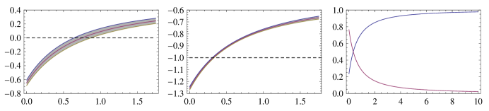
Figure 1: The evolution curves of $q(z)$ (left panel), $w^{eff}_{\Lambda}(z)$ (central panel) with $1\sigma$ error region and dimensionless parameters $\Omega_{m}(z)$ and $\Omega_{\Lambda}(z)$ (right panel) with respect to redshift $z$ where the best fit values are adopted.

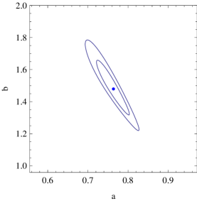
Figure 2: The contours in the planes of $a-b$ with $1\sigma$ and $2\sigma$ regions. The central dots denote the best fit values of model parameters.

Clearly, with this simple parameterized form of $c^{2}$, an observational consistent model is presented when the Hubble horizon is taken as the role of an IR cut-off in the holographic dark energy scenario. For the introduction of an extra term in the effective EoS of the vacuum energy density of time variable cosmological constant, the cosmological constant boundary crossing can be realized, as seen in the central panel of Fig. 1. One can also see that the effective EoS of time variable CC is phantom-like at present.

IV Conclusions

In this paper, time variable CC is explored when the Hubble horizon is taken as the role of an IR cut-off, i.e. $\Lambda(t)=3c^{2}H^{2}(t)$ which corresponds to the vacuum energy density $\rho_{\Lambda}=3c^{2}M^{2}_{P}H^{2}$. When $c$ is a fixed constant, a scaling solution is obtained. If $c$ is in the range of $1/3<c^{2}<1$, an accelerated expansion universe can exist. But, unfortunately with this fixed gap filling constant $c$, no-transition from decelerated expansion to accelerated expansion can be realized. However, the Hubble horizon is a natural choice of cosmological length scale. To realize an accelerated expansion universe, a transition from the past decelerated expansion to recent accelerated expansion and cosmic observational compatible model in the case of Hubble horizon as an IR cut-off, a time or scale dependent gap filling constant $c$ is considered. With this time or scale dependent $c$, a time or scale dependent dimensionless energy density is derived. And, the effective EoS of time variable CC gains an term which can make it cross cosmological constant boundary and be phantom-like at present. By giving a simple parameterized form of $c^{2}$ as an example, the model was confronted by cosmic observations which include SN Ia, BAO and CMB shift parameter $R$. The constraint result shows that a cosmic observational compatible model can be realized in this framework when the Hubble horizon is taken as the role of an IR cut-off. That can be seen from the Fig. 1. However, we do not know the first principle or fundamental physics theory to give the form of time or scale dependent $c(a)$. It seems the limitation of our model. But, we expect this consideration can shed light on the study of holographic dark energy models.

Appendix A Cosmic Observational Constraints

In this section, cosmic observations and methods used in this paper are described.

A.1 SN Ia

We constrain the parameters with the Supernovae Cosmology Project (SCP) Union sample including $307$ SN Ia ref:SCP , which is distributed over the redshift interval $0.015\leq z\leq 1.551$. Constraints from SN Ia can be obtained by fitting the distance modulus $\mu(z)$ ref:smallomega ; ref:BDSN1 ; ref:BDSN2 ; ref:BDSN3 ; ref:JCAPXU ; ref:SNchi2

$$\mu_{th}(z)=5\log_{10}(D_{L}(z))+\mu_{0},$$ (32)

where, $D_{L}(z)$ is the Hubble free luminosity distance $H_{0}d_{L}(z)/c$ and

$$d_{L}(z) = c(1+z)\int_{0}^{z}\frac{dz^{\prime}}{H(z^{\prime})}$$ (33)

$$\mu_{0} \equiv 42.38-5\log_{10}h,$$ (34)

where $H_{0}$ is the Hubble constant which is written in terms of a re-normalized quantity $h$ defined as $H_{0}=100h~{}{\rm km~{}s}^{-1}{\rm Mpc}^{-1}$. The observed distance moduli $\mu_{obs}(z_{i})$ of SN Ia at $z_{i}$ is

$$\mu_{obs}(z_{i})=m_{obs}(z_{i})-M,$$ (35)

where $M$ is their absolute magnitudes.

For the SN Ia dataset, the best fit values of parameters $p_{s}$ in the model can be determined by a likelihood analysis based on the calculation of

$$\chi^{2}(p_{s},M^{\prime}) \equiv \sum_{SN}\frac{\left[\mu_{obs}(z_{i})-\mu_{th}(p_{s},z_{i})\right]^{2}}{\sigma_{i}^{2}}$$ (36)

$$= \sum_{SN}\frac{\left[5\log_{10}(D_{L}(p_{s},z_{i}))-m_{obs}(z_{i})+M^{\prime}\right]^{2}}{\sigma_{i}^{2}},$$

where $M^{\prime}\equiv\mu_{0}+M$ is a nuisance parameter which includes the absolute magnitude and $h$. The nuisance parameter $M^{\prime}$ can be marginalized over analytically ref:SNchi2 ,

$$\bar{\chi}^{2}(p_{s})=-2\ln\int_{-\infty}^{+\infty}\exp\left[-\frac{1}{2}\chi^{2}(p_{s},M^{\prime})\right]dM^{\prime},$$ (37)

to arrive at

$$\bar{\chi}^{2}=A-\frac{B^{2}}{C}+\ln\left(\frac{C}{2\pi}\right),$$ (38)

where

$$A=\sum_{SN}\frac{\left[5\log_{10}(D_{L}(p_{s},z_{i}))-m_{obs}(z_{i})\right]^{2}}{\sigma_{i}^{2}},$$ (39)

$$B=\sum_{SN}\frac{5\log_{10}(D_{L}(p_{s},z_{i})-m_{obs}(z_{i})}{\sigma_{i}^{2}},$$ (40)

$$C=\sum_{SN}\frac{1}{\sigma_{i}^{2}}\;.$$ (41)

Eq. (36) has a minimum at the nuisance parameter value $M^{\prime}=B/C$ which contains information of the values of $h$ and $M$. That is to say, one can find the values of $h$ and $M$ when one of them is known. However, in the literatures ref:smallomega ; ref:BDSN1 ; ref:BDSN2 ; ref:BDSN3 ; ref:JCAPXU ; ref:SNchi2 , the expression

$$\chi^{2}_{SN}(p_{s},B/C)=A-(B^{2}/C)$$ (42)

is used usually in the likelihood analysis, which is up to a constant to Eq. (38). In this case, the results will not be affected when the distribution of $M^{\prime}$ is flat.

A.2 BAO

The BAO are detected in the clustering of the combined 2dFGRS and SDSS main galaxy samples, and measure the distance-redshift relation at $z=0.2$. BAO in the clustering of the SDSS luminous red galaxies measure the distance-redshift relation at $z=0.35$. The observed scale of the BAO calculated from these samples and from the combined sample are jointly analyzed using estimates of the correlated errors, to constrain the form of the distance measure $D_{V}(z)$ ref:Okumura2007 ; ref:Eisenstein05 ; ref:Percival1 ; ref:Percival2

$$D_{V}(z)=\left[(1+z)^{2}D^{2}_{A}(z)\frac{cz}{H(z)}\right]^{1/3},$$ (43)

where $D_{A}(z)$ is the proper (not comoving) angular diameter distance, which has the following relation with $d_{L}(z)$

$$D_{A}(z)=\frac{d_{L}(z)}{(1+z)^{2}}.$$ (44)

Matching the BAO to have the same measured scale at all redshifts then gives ref:Percival2

$$D_{V}(0.35)/D_{V}(0.2)=1.736\pm 0.065.$$ (45)

Then, the $\chi^{2}_{BAO}(p_{s})$ is given as

$$\chi^{2}_{BAO}(p_{s})=\frac{\left[D_{V}(0.35)/D_{V}(0.2)-1.736\right]^{2}}{0.065^{2}}.$$ (46)

A.3 CMB shift Parameter R

The CMB shift parameter $R$ is given by ref:Bond1997

$$R(z_{\ast})=\sqrt{\Omega_{m}H^{2}_{0}}(1+z_{\ast})D_{A}(z_{\ast})/c$$ (47)

which is related to the second distance ratio $D_{A}(z_{\ast})H(z_{\ast})/c$ by a factor $\sqrt{1+z_{\ast}}$. Here the redshift $z_{\ast}$ (the decoupling epoch of photons) is obtained by using the fitting function Hu:1995uz

$$z_{\ast}=1048\left[1+0.00124(\Omega_{b}h^{2})^{-0.738}\right]\left[1+g_{1}(\Omega_{m}h^{2})^{g_{2}}\right],$$ (48)

where the functions $g_{1}$ and $g_{2}$ are given as

$$g_{1} = 0.0783(\Omega_{b}h^{2})^{-0.238}\left(1+39.5(\Omega_{b}h^{2})^{0.763}\right)^{-1},$$ (49)

$$g_{2} = 0.560\left(1+21.1(\Omega_{b}h^{2})^{1.81}\right)^{-1}.$$ (50)

The 5-year WMAP data of $R(z_{\ast})=1.710\pm 0.019$ ref:Komatsu2008 will be used as constraint from CMB, then the $\chi^{2}_{CMB}(p_{s})$ is given as

$$\chi^{2}_{CMB}(p_{s})=\frac{(R(z_{\ast})-1.710)^{2}}{0.019^{2}}.$$ (51)

References

- (1) A.G. Riess, et al., Astron. J. 116 1009(1998) [astro-ph/9805201].
- (2) S. Perlmutter, et al., Astrophys. J. 517 565(1999) [astro-ph/9812133].
- (3) D.N. Spergel et.al., Astrophys. J. Suppl. 148 175(2003) [astro-ph/0302209].
- (4) D.N. Spergel et al., Astrophys. J. Suppl.170 377(2007) [astro-ph/0603449].
- (5) M. Tegmark et.al., Phys. Rev. D 69 (2004) 103501 [astro-ph/0310723].
- (6) M. Tegmark et.al., Astrophys. J. 606 (2004) 702 [astro-ph/0310725].
- (7) E. Komatsu et.al., Astrophys. J. Suppl. 180, 330 (2009) [arXiv:0803.0547].
- (8) S.D.H. Hsu, Phys. Lett. B594 13(2004) [arXiv:hep-th/0403052].
- (9) M. Li, Phys. Lett. B603 1(2004) [hep-th/0403127]; Q.G. Huang and M. Li, JCAP 03, 001 (2005) [hep-th/0410095]; Q.G. Huang and M. Li, JCAP 08, 013 (2004) [astro-ph/0404229]; B. Chen, M. Li and Y. Wang, Nucl. Phys. B 774, 256 (2007) [astro-ph/0611623]; J.F. Zhang, X. Zhang and H.Y. Liu, Eur. Phys. J.C 52 693(2007) [arXiv:0708.3121]; S. Nojiri, S.D. Odintsov, Gen. Rel. Grav. 38 1285(2006);
- (10) P. Horava, D. Minic, Phys. Rev. Lett. 85 1610(2000).
- (11) R. Horvat, Phys. Rev. D70 087301(2004).
- (12) Y. Gong, Phys. Rev. D 61 (2000) 043505.
- (13) Y. Gong, Phys. Rev. D 70 (2004) 064029.
- (14) M. R. Setare, Phys. Lett. B644 99(2007).
- (15) N. Banerjee, D. Pavon, Phys. Lett. B 647 447(2007).
- (16) B. Nayak, L. P. Singh, [arXiv:0803.2930].
- (17) L. Xu, W. Li, J. Lu, Eur. Phys. J. C 60 135 (2009).
- (18) C.J. Feng, Phys. Lett. B 663 367(2008).
- (19) L. Xu, W. Li, J. Lu, arXiv:0905.4772; L. Xu, J. Lu, W. Li, arXiv:0905.4773.
- (20) B. Wang, C.Y. Lin, E.o Abdalla, Phys. Lett. B 637 357(2006); H. Kim, H.W. Lee, Y.S. Myung, Phys. Lett. B 632 605(2006); B. Hu, Y. Ling, Phys. Rev. D 73 123510(2006); W. Zimdahl, D. Pavon, [arXiv:astro-ph/0606555]; H.M. Sadjadi, JCAP 02 026(2007); M.R. Setare, E.C. Vagenas, Int. J. Mod. Phys. D 18 147(2009); Q. Wu, Y. Gong, A. Wang, J.S. Alcaniz, [arXiv:0705.1006]; J.F. Zhang, X. Zhang, H.Y. Liu, Phys. Lett. B 659 26(2008); C. Feng, B. Wang, Y. Gong, R.K. Su, [arXiv:0706.4033]; S.F. Wu, P.M. Zhang, G.H. Yang, Class. Quan. Grav. 26 055020(2009); M. A. Rashid, M. U. Farooq, M. Jamil, [arXiv:0901.3724].
- (21) D. Pavon, W. Zimdahl, Phys. Lett. B 628 206(2005).
- (22) L. Xu, W. Li, J. Lu, arXiv:0905.4552; L. Xu, J. Lu, B. Chang, Chapter 1. Dark Energy-Current Advances and Ideas, Edited by Dr. Jeong Ryeol Choi; J. Lu, L. Xu, J. Li, H. Liu, Mod. Phys. Lett. A 23, 2067(2008); L. Xu, J. Lu, Mod. Phys. Lett. A 24, 369(2009); L. Xu, H. Liu, Mod. Phys. Lett. A 23, 1939(2008).
- (23) M. Kowalski et al., Astrophys. J. 686, 749(2008) [arXiv:0804.4142].
- (24) V. Acquaviva, L. Verde, JCAP 12 001(2007) [arXiv:0709.0082].
- (25) A. Riazuelo, J. Uzan, Phys.Rev. D66 023525(2002) [arXiv:astro-ph/0107386].
- (26) E. Garcia-Berro, E. Gaztanaga, J. Isern, O. Benvenuto, L. Althaus, [arXiv:astro-ph/9907440].
- (27) S. Nesseris, L. Perivolaropoulos, Phys. Rev. D73 103511(2006) [arXiv:astro-ph/0602053].
- (28) L. Xu, W. Li, J. Lu, JCAP 0907 031(2009).
- (29) S. Nesseris and L. Perivolaropoulos, Phys. Rev. D 72, 123519 (2005) [arXiv:astro-ph/0511040]; L. Perivolaropoulos, Phys. Rev. D 71, 063503 (2005) [arXiv:astro-ph/0412308]; S. Nesseris and L. Perivolaropoulos, JCAP 02, 025 (2007) [arXiv:astro-ph/0612653]; E. Di Pietro and J. F. Claeskens, Mon. Not. Roy. Astron. Soc. 341, 1299 (2003) [arXiv:astro-ph/0207332]; A.C.C. Guimaraes, J.V. Cunha and J.A.S. Lima, [arXiv:0904.3550].
- (30) T. Okumura, T. Matsubara, D. J. Eisenstein, I. Kayo, C. Hikage, A. S. Szalay and D. P. Schneider, ApJ 676, 889(2008) [arXiv:0711.3640]
- (31) D. J. Eisenstein, et al, Astrophys. J. 633, 560 (2005) [astro-ph/0501171].
- (32) W.J. Percival, et al, Mon. Not. Roy. Astron. Soc., 381, 1053(2007) [arXiv:0705.3323].
- (33) W.J. Percival, et al, arXiv:0907.1660 [astro-ph.CO].
- (34) J. R. Bond, G. Efstathiou, and M. Tegmark, MNRAS 291 L33(1997).
- (35) W. Hu, N. Sugiyama, Astrophys. J. 471 542(1996) [astro-ph/9510117].
- (36) E. Komatsu, et.al., Astrophys. J. Suppl. 180, 330(2009) [arXiv:0803.0547].