The Piranha algebraic manipulator

Abstract

In this paper we present a specialised algebraic manipulation package devoted to Celestial Mechanics. The system, called Piranha, is built on top of a generic and extensible framework, which allows to treat efficiently and in a unified way the algebraic structures most commonly encountered in Celestial Mechanics (such as multivariate polynomials and Poisson series). In this contribution we explain the architecture of the software, with special focus on the implementation of series arithmetics, show its current capabilities, and present benchmarks indicating that Piranha is competitive, performance-wise, with other specialised manipulators.

1 Introduction

Since the late Fifties ([27]) researchers in the field of Celestial Mechanics have manifested a steady and constant interest in software systems able to manipulate the long algebraic expressions arising in the application of perturbative methods. Despite the widespread availability of commercial general-purpose algebraic manipulators, researchers have often preferred to develop and employ specialised ad-hoc programs (we recall here, without claims of completeness, [10], [31, 32], [48], [7], [4], [18], [47], [1], [29], [13, 12] and [23]). The reason for this preference lies mainly in the higher performance that can be obtained by these. Specialised manipulators are built to deal only with specific algebraic structures, and thus they can adopt fast algorithm and data structures and avoid the overhead inherent in general-purpose systems (which instead are designed to deal with a wide variety of mathematical expressions). The performance gap between specialised and general-purpose manipulators is often measured in orders of magnitude, especially for the most computationally-intensive operations.

The need for computer-assisted algebraic manipulation in Celestial Mechanics typically arises in the context of perturbative methods. In classical perturbative approaches, for instance, the equations of motion of celestial bodies are expanded into Fourier series having power series of “small” quantities (e.g., orbital eccentricity, orbital inclination, ratio of the masses) as coefficients. This algebraic structure, commonly referred to as Poisson series, allows to identify the terms relevant to the specific physical problem being considered and apply adequate methods of solution of the equations of motion ([42], Chapters 7 and 8). Likewise, in the computation of normal forms in studies of dynamical systems the Hamiltonian is commonly expanded into power series, hence leading to multivariate polynomial algebraic expressions ([33]). Another example is the computation of the tide-generating potential ([19, 50]), which involves the manipulation of Fourier series with numerical coefficients.

In order to give a simple example, we recall here that classical perturbative methods employ Fourier series expansions like this one ([42], Chapter 2),

$$\cos f=\cos M+e\left(\cos 2M-1\right)+\frac{9}{8}e^{2}\left(\cos 3M-\cos M\right)\\ +\frac{4}{3}e^{3}\left(\cos 4M-\cos 2M\right)\\ +e^{4}\left(\frac{25}{192}\cos M-\frac{225}{128}\cos 3M+\frac{625}{384}\cos 5M\right),$$ (1)

which represents the expansion of the cosine of the true anomaly $f$ of the orbit of a celestial body in terms of cosines of the mean anomaly $M$ up to fourth order in the eccentricity $e$. Such series are manipulated and combined with other series through operations such as addition, subtraction, multiplication, differentiation and symbolic substitution, leading to a final Fourier series representing the perturbing potential.

All the mentioned applications require the ability to perform simple operations on series whose number of elements can grow remarkably large. In modern studies on the long-term stability of the Solar System, for instance, researchers have to deal with series of millions of terms ([37]). The fact that in many cases it is possible to perform the most computationally-intensive calculations within the form of a single algebraic structure might explain the persisting interest in specific algebraic manipulators.

To improve performance with respect to general-purpose systems, different specialised manipulators adopt similar techniques which are a natural exploitation of the characteristics of the problems that they are built to tackle. Exponents in polynomials, for instance, are usually represented as hardware integers, instead of the arbitrary-size integers employed in general-purpose systems. Perturbative methods, indeed, assume that the quantities subject to exponentiation are small, so that in practice the exponents encountered in such calculations have values below $10^{2}$ (but usually they are lower). Similarly, when calculating the harmonic expansion of the tide-generating potential it is often sufficient to represent the series’ coefficients as standard double-precision floating point variables, whereas general-purpose manipulators must be able to operate with multiprecision floating point arithmetic and thus incur in an overhead that is unnecessary from the point of view of the celestial mechanician.

The work presented here has four major objectives:

1. to define a framework able to handle concisely and in a generalised fashion the algebraic structures most commonly encountered in Celestial Mechanics,

2. to identify and implement efficient algorithms and data structures for the manipulation of said algebraic structures,

3. to provide means to interact effectively and flexibly with the computational objects, and

4. to provide an open system promoting participation and extensibility.

We feel that many of the previous efforts in the field of algebraic manipulators devoted to Celestial Mechanics have failed in at least one of these objectives. Many manipulators, for instance, have been written for very specific tasks, so that it can be difficult to extend or reuse them in other contexts. Others employ algorithms and data structures whose performance is not optimal. Yet others are fast and full-featured, but they are not open.

While the work presented here is still in progress, preliminary benchmarks seem to indicate that our system, called Piranha, is competitive performance-wise with other more mature systems. In this contribution we illustrate Piranha’s architecture and its most noteworthy implementation details, with special emphasis on series arithmetic. We also present a brief overview of the Python interface and expound on benchmarks. Finally, we discuss the future direction of the project, including desirable features not yet implemented and possible performance improvements.

2 Algebraic structures in Celestial Mechanics

As hinted in the introduction, Celestial Mechanics employs diverse algebraic structures in the form of series. Multivariate polynomials appear naturally in perturbation theories in the form

$$\sum_{\mathbf{i}}C_{\mathbf{i}}\mathbf{x}^{\mathbf{e}_{\mathbf{i}}},$$ (2)

where we have adopted the convention

$$\mathbf{x}^{\mathbf{e}_{\mathbf{i}}}=x_{0}^{e_{i_{0}}}x_{1}^{e_{i_{1}}}\ldots x_{n-1}^{e_{i_{n-1}}}$$ (3)

with $\mathbf{i}=\left(i_{0},i_{1},\ldots,i_{n-1}\right)$ an integer multiindex, $\mathbf{e}_{\mathbf{i}}$ a vector of integer exponents indexed over $\mathbf{i}$, $C_{\mathbf{i}}$ a numerical coefficient indexed over $\mathbf{i}$ and $\mathbf{x}=\left(x_{0},x_{1},\ldots,x_{n-1}\right)$ a vector of symbolic variables. Although in perturbation theories series expansions have infinite terms, in practical calculations series are truncated to some finite order, so that the components of the $\mathbf{i}$ vectors vary on finite ranges. Please note that, strictly speaking, formula (2) represents a superset of multivariate polynomials, since the $\mathbf{e}_{\mathbf{i}}$’s components are allowed to assume negative values. It is hence more correct to refer to expressions in the form of (2) as multivariate Laurent series, as pointed out in [51]. Nevertheless, when referring to polynomials from now on we will encompass also Laurent series.

In Celestial Mechanics another commonly-encountered algebraic structure is the so-called Poisson series ([17])

$$\sum_{\mathbf{i}}\sum_{\mathbf{j}}C_{\mathbf{ij}}\mathbf{x}^{\mathbf{e}_{\mathbf{i}\mathbf{j}}}\begin{array}[]{c}\cos\\ \sin\end{array}\left(\mathbf{t}\cdot\mathbf{i}\right),$$ (4)

which consists of a multivariate Fourier series in the trigonometric variables $\mathbf{t}$ with multivariate Laurent series as coefficients. We refer to the elements of the integer vector $\mathbf{i}$ as trigonometric multipliers. In practical applications it is sometimes convenient to represent the trigonometric parts of Poisson series through complex exponentials, hence defining a structure which we refer to as polar Poisson series:

$$\sum_{\mathbf{i}}\sum_{\mathbf{j}}C_{\mathbf{ij}}\mathbf{x}^{\mathbf{e}_{\mathbf{i}\mathbf{j}}}\exp\left[\imath\left(\mathbf{t}\cdot\mathbf{i}\right)\right],$$ (5)

where $\imath=\sqrt{-1}$. Poisson series arise routinely in the formulation of the gravitational disturbing function, where the symbolic variables represent the orbital elements of celestial bodies ([42], Chapter 6).

The subset of degenerate Poisson series with purely numerical coefficients is often referred to simply as Fourier series:

$$\sum_{\mathbf{i}}C_{\mathbf{i}}\begin{array}[]{c}\cos\\ \sin\end{array}\left(\mathbf{t}\cdot\mathbf{i}\right).$$ (6)

Fourier series are used to express the periodic solutions of theories of motion of celestial bodies. They are often employed in problems involving the harmonic expansion of the tide-generating potential, where the theories of motion of celestial bodies are plugged into the expression of the potential and manipulated in order to be obtain a formulation of the potential in Fourier series form.

Poisson series can be seen as a subset of echeloned Poisson series, which are defined by the following formula:

$$\sum_{\mathbf{i}}\sum_{\mathbf{j}}\sum_{\mathbf{k}}C_{\mathbf{ijk}}\mathbf{x}^{\mathbf{e}_{\mathbf{i}\mathbf{j}\mathbf{k}}}\frac{1}{\prod_{\mathbf{l}}\left(\mathbf{d}\cdot\mathbf{m}_{\mathbf{i}\mathbf{j}\mathbf{l}}\right)^{\delta_{\mathbf{i}\mathbf{j}\mathbf{l}}}}\begin{array}[]{c}\cos\\ \sin\end{array}\left(\mathbf{t}\cdot\mathbf{i}\right),$$ (7)

where $\mathbf{d}$ is a vector of symbolic variables (the so-called divisors), $\mathbf{m}$ a vector of integers indexed over the multiindices $\mathbf{i}$, $\mathbf{j}$ and $\mathbf{l}$, and $\delta_{\mathbf{i}\mathbf{j}\mathbf{l}}$ a positive integer value, again indexed over $\mathbf{i}$, $\mathbf{j}$ and $\mathbf{l}$. Echeloned Poisson series are employed, for instance, in lunar theories, where it is necessary to express symbolically the frequencies of the trigonometric variables. Such frequencies appear as divisors when integrating the equations of motion with respect to time. While Poisson series manipulators are relatively common, echeloned Poisson series manipulators are less widespread ([49], [30]).

There are other less common algebraic structures for which specialised algebaric manipulators exist. We recall here the mainpulator described in [43], which targets Earth rotation theories and handles a superset of echeloned Poisson series called Kinoshita series.

In order to accomodate all the aforementioned algebraic structures, Piranha adopts a definition of series based on the following concepts:

Definition 1.

Terms are pairs constituted by a coefficient and a key.

Definition 2.

Two terms are considered equivalent if and only if their keys are.

Definition 3.

Series are sets of terms.

Such concepts allow to introduce a recursive definition of series which is exemplified in Figure 1, and which was inspired by the definition of echeloned Poisson series in [49].

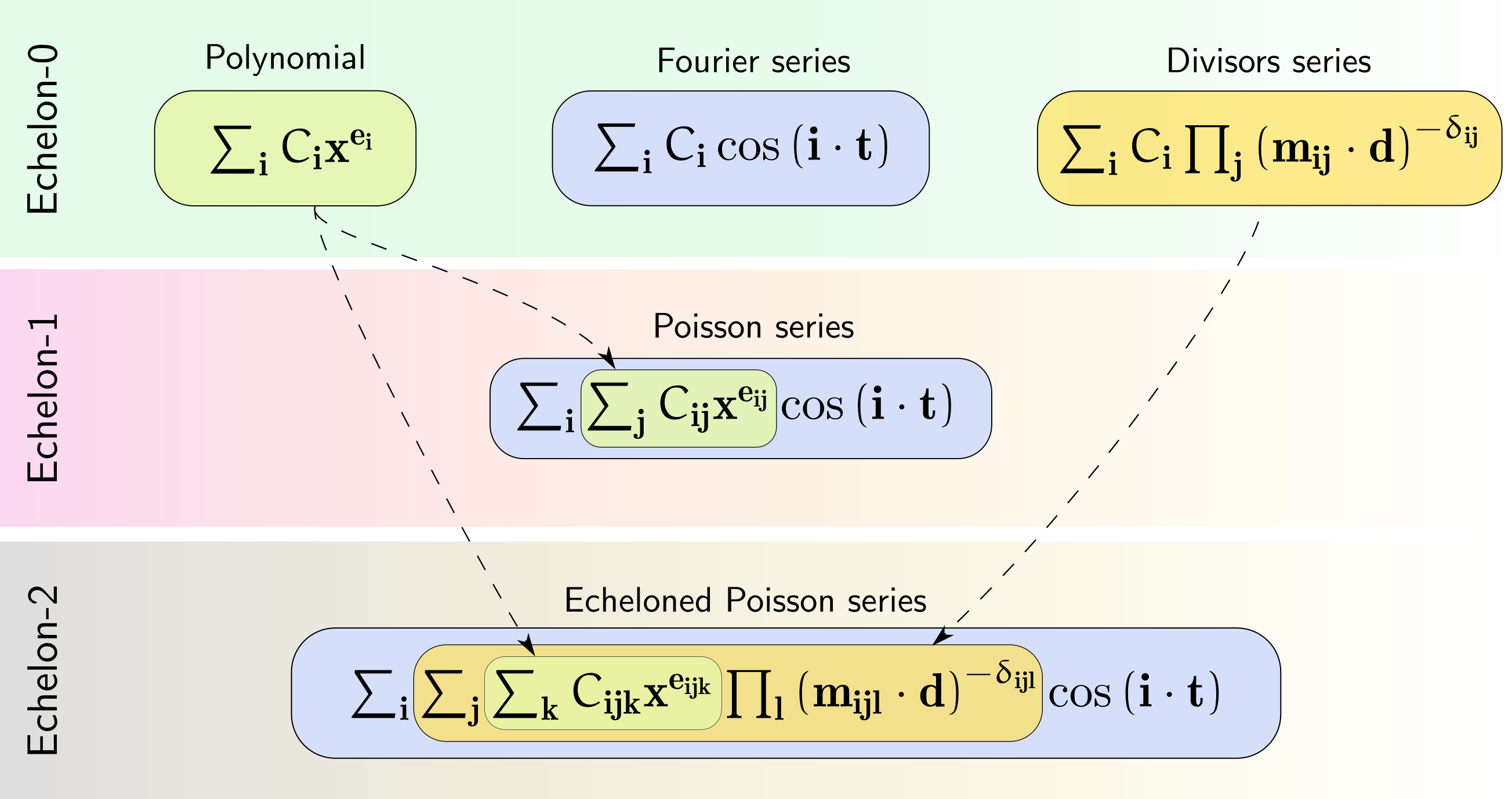
Figure 1: Definition of series in Piranha. Echelon-0 series are series with numerical coefficients, echelon-$n$ series with $n>0$ are series with echelon-$\left(n-1\right)$ series as coefficients.

The lowest level of this scheme is populated by series whose coefficients are numerical, such as Fourier series (where we find trigonometric keys) and polynomials (where keys are multivariate monomials). This level represents the terminal point of the recursion and we refer to it as echelon-0. The next level, echelon-1, features series whose coefficients are echelon-0 series, and it is populated by Poisson series (in both their traditional and polar forms). Similarly echelon-2, featuring echeloned Poisson series, is characterised by series whose coefficients are echelon-1 series. The following generalisation now follows straightforwardly:

Definition 4.

Echelon-0 series are series with numerical values as coefficients.

Definition 5.

Echelon-$n$ series are series with echelon-$\left(n-1\right)$ series as coefficients.

At the present time, Piranha implements Fourier series, polynomials and Poisson series, with various possible combinations for the representation of numerical coefficients and keys. In our opinion, one of the key advantages of this framework is that it allows to treat different algebraic structures in a unified way and without any overhead. While it is possible, for instance, to use a Poisson series manipulator to operate on multivariate polynomials and Fourier series, this approach incurs in a performance penalty related to the unnecessary management of empty trigonometric keys and monomials, respectively. By using the framework described here, it is instead possible to build specialised manipulators with little effort.

3 A generically-programmed architecture

In order to implement in an efficient and concise way the recursive scheme described in §2, we have chosen to adopt a programming paradigm which is both generic and object-oriented. The kind of genericity we seek is twofold:

1. we want to be able to implement series types with different representations for coefficients and keys. When undertaking the task of the development of the disturbing function in planetary problems, for instance, it may be desirable to operate with multiprecision rational numbers as coefficients, in order to retain maximum precision. Likewise, in certain problems it may be enough to operate with polynomial exponents or trigonometric multipliers represented as 16 or even 8 bits integers as opposed to word-size integers, so that it is possible to adopt a more compact representation for keys in such cases;

2. consequently, we want to be able to write algorithms for the manipulation of terms once and for all the different combinations of coefficients and keys, at the same time retaining the ability to specialise the algorithms under certain circumstances.

The ultimate goal is to minimise code duplication and keep the source code as compact as possible. In a sense, we perceive Piranha as an attempt to implement the algebraic manipulation framework envisioned in [26].

Our language of choice for the implementation of Piranha’s architecture is C++, in its flavour that is sometimes referred to as modern C++ (a term first popularised in [2]). This programming paradigm uses extensively C++ templates to achieve genericity at compile-time and to provide metaprogramming capabilities (meaning that the program is able to modify itself and automatically generate source code at compile-time). Modern C++ can be used to provide container classes where the type of the contained items is parametrised, to enable a type of polymorphism which is entirely resolved at compile-time (in contrast to the runtime polymorphism of traditional C++), and to write algorithms able to operate on generic types. Since template metaprogramming operates during the compilation of the program, its overhead at runtime is null, and thus it is particularly appealing in those contexts, such as scientific computing, where performance is paramount.

In Piranha, series are represented as template classes with coefficients and keys as parametrised types. A base series class provides the bulk of low-level operations on series. Base series are not intended to be used directly, instead they serve as a foundation for two other series classes, i.e., named series and coefficient series. Named series are intended to be employed directly by the user, and they are so called because they embed a description of their arguments in a $n$-tuple of vectors (where $n$ is the echelon level plus one). The series types described in §2 are all named series. Coefficient series, as the name suggests, are instead series serving as coefficients in other series. Laurent series as coefficients in Poisson series are an example of coefficient series.

All the series classes implemented in Piranha inherit from the base series class and either from the named series class or the coefficient series class. A minimal series class defined this way is able to read and save series files, to interact with plain old C++ data types (i.e., integers and double-precision values), to produce a numerical evaluation of itself based on the substitution of arguments with numerical values and to perform series addition and subtraction. The capabilities of the series are then augmented, again through multiple inheritance, by the use of additional classes which we refer to as toolbox classes. Toolboxes are used to provide routines for more advanced tasks such as series multiplication, exponentiation to real powers, trigonometric functions, special functions, series expansions relevant to Celestial Mechanics and so on, and also to group together methods relevant only to specific series types. Toolboxes are also used to provide those capabilities expected from series with complex coefficients and which are useless in series with real coefficients, such as the extraction of real and imaginary parts and full arithmetical interoperability between complex and real series.

As an example, the Poisson series class at the present times inherits from the following classes: base series, named series, series multiplication toolbox, power series toolbox, special functions toolbox, Celestial Mechanics toolbox and common Poisson series toolbox.

Toolboxes are generically programmed and may cross-reference each other. The special functions toolbox, for instance, requires the presence of a series multiplication toolbox (which might be already provided by the framework, but which can also be (re)implemented by the user); if the series multiplication toolbox is not available, a compile-time error will be produced. To avoid runtime overhead, the system of toolboxes extensively employs a design pattern known as curiously-recurring template pattern ([15]). This approach avoids runtime virtual-table lookups by achieving a form of polymorphism which is resolved entirely at compile-time (and which has been sometimes referred to as static polymorphism).

At the time of this writing, Piranha supports the following coefficients types:

1. standard double-precision floating-point,

2. multiprecision integers,

3. multiprecision rationals,

and their complex counterparts. The multiprecision coefficients use the GMP bignum library ([54]). The supported key types are:

1. dynamically-sized trigonometric array (for Fourier and Poisson series),

2. dynamically-sized multivariate monomial array (for polynomials).

For both keys the user may choose as integer size either 8 or 16 bits at compile-time. Considering that Piranha currently supports three named series types (polynomials and Poisson/Fourier series), there are tens of possible manipulators implementable with a one-line type definition. The following statement, for instance, defines a Fourier series class called dfs with double-precision floating-point coefficients and 16 bits trigonometric keys:

⬇

typedef fourier_series<double_cf, trig_array<16> > dfs;

In order to evaluate the global impact of the framework, we have run a simple SLOC (single line of code) analysis on Piranha and on two freely-available specialised manipulators called Gregoire and Colbert ([13], [12]) which target Fourier series (Gregoire) and Poisson series (Colbert) with floating-point coefficients. Gregoire and Colbert, whose feature set is comparable to Piranha’s, are written in Fortran and they consist of around $4\,000$ SLOCs each. By comparison Piranha’s SLOC count is about $10\,000$, but, as pointed out earlier, Piranha really implements many manipulators with different characteristics and different representations for coefficients and keys. Another interesting detail of our simple SLOC analysis is that around 70% of Piranha’s source code is shared among all the available series types.

4 Storage of terms

Series appearing in the context of Celestial Mechanics are generally sparse. By this we mean that, given finite upper and lower boundaries for the multiindices indexing the series described in §2, most of the possible multiindices combinations will be associated to null terms. This is the main reason that led us to choose hashing as storage method for series in Piranha.

We recall here briefly that hashing is an indexing technique based on a hash function that maps the items to be stored to integer values (hash values). Such values are used as indices in array-like structures called hash tables (sometimes called also dictionaries). The choice of the hash function, the strategy of collision resolution (i.e., how to cope with different items hashing to the same value), the resize policy, all contribute to the performance of the hash table and they are thoroughly analysed in standard computer science textbooks such as [35] and [16]. We just recall that, when properly implemented, hash tables feature expected $\operatorname{O}\!\left(1\right)$ complexity for lookup, insertion and deletion of elements.

Given the definition of series provided in §2, it readily follows that, since terms are uniquely identified by their keys, the hash function will take the term’s key as argument and that coefficients have no role in the identifcation of a term. The presently-supported key types (i.e., trigonometric keys and multivariate monomials) can be seen as sequences of integers, with the flavour of trigonometric keys (i.e., sine or cosine) codified as a boolean flag:

$$\cos\left(x+2y-3z\right) \Longrightarrow \left[1,2,-3,\textnormal{true}\right],$$ (8)

$$\sin\left(x-z\right) \Longrightarrow \left[1,0,-1,\textnormal{false}\right],$$ (9)

$$x^{3}y^{4}z^{-5} \Longrightarrow \left[3,4,-5\right].$$ (10)

At the present time, Piranha implements the supported key types as dynamically-sized dense arrays, meaning that the integer values are stored in contiguous memory areas allocated dynamically and that null values are explicitly stored. This type of representation is referred to as distributed in the literature, as opposed to the recursive representation in which $n$-variate series are recursively represented as $\left(n-1\right)$-variate series with univariate series as coefficients (see [53] for a comparison of polynomial representations in computer algebra systems).

Both trigonometric keys and monomials are implemented on top of a base class called int_array, which provides common low-level functionality. Since, as mentioned earlier, we don’t need the full range of word-size integers for the representation of keys, int_array employs an integer packing technique to store multiple sub-word-size integers into a word-size integer. The user can choose a size for the packed integers of either 8 or 16 bits at compile-time. The data layout of a multivariate monomial in eight variables on a 64 bits architecture with packed integer size of 16 bits will then look like this:

$$\underbrace{\begin{array}[]{cccc}\underbrace{n_{0}}_{16\textnormal{ bits}}&n_{1}&n_{2}&n_{3}\end{array}}_{64\textnormal{ bits}}\underbrace{\begin{array}[]{cccc}\underbrace{n_{4}}_{16\textnormal{ bits}}&n_{5}&n_{6}&n_{7}\end{array}}_{64\textnormal{ bits}}$$

By using a C union it is possible to acces the memory space as an array of either word-size or packed-size integers. In addition to saving memory, this approach also allows to increase the performance of those operations which can work on multiple values independently; when comparing two keys, for instance, we can compare directly the word-size integers, hence avoiding the overhead of looping on the packed values and performing the comparison of multiple packed integers in one pass. Similarly, it is possible to compute the hash value of the key by combining (or mixing) the word-size integers instead of the packed integers.

At the present time, Piranha relies on the hashing facilities provided by the Boost C++ libraries ([5]). Boost’s hash_combine function is based on a family of hash functions described in [46], initially conceived for string hashing. This class of hash functions is refferred to as shift-add-xor because at each step of the iteration for the calculation of the hash value, operations of bit shifting, addition and bitwise exclusive OR are used. In Piranha the first word-size integer of each key is used as a seed value and then mixed with the other word-size integers of the key. For trigonometric keys, additional mixing is provided by the flavour of the key (cast as an integer value). The hash value is then used to store the term in a Boost hash_set data structure. This hashing container is a fairly standard hash set which uses prime numbers as sizes and the modulo operation for extracting a useful index from the hash value, and which employs separate chaining for collision resolution.

The single point of entry for terms in the base series class is the insert() method. This method is a wrapper around hash_set’s own insert() method which performs additional checks before actually inserting the term into the container. The most important checks are the following (in order of execution):

1. term is ignorable: a term is always ignorable when either the coefficient or the key are mathematically equivalent to zero. Additionally, coefficients and keys may implement additional ignorability criterions (double-precision coefficients, for instance, are considered ignorable when their absolute value is below a critical numerical threshold). Ignorable terms are simply discarded;

2. term is in canonical form: the keys of certain series types might have multiple valid mathematical representations. The two trigonometric keys

   $$\cos\left(x-y\right),$$

   $$\cos\left(-x+y\right),$$

   for instance, are mathematically equivalent, yet their straightforward translations into an array-like container will be different:

   $$\left[1,-1,\textnormal{true}\right],$$

   $$\left[-1,1,\textnormal{true}\right].$$

   To remove such ambiguity, trigonometric keys, if necessary, are reduced during insertion to a unique canonical representation in which the first integer element is always positive (in case of sine trigonometric keys the canonicalisation of the key must be followed by a change in the sign of the coefficient);

3. term is not unique: before insertion of a non-ignorable term in canonical form it is checked whether an equivalent term exists in the series. This operation requires a lookup operation in the hash_set. If an equivalent term exists, the coefficient of the term being inserted is added to the existing equivalent term. Otherwise, the term is inserted as a new element.

The base series’ insert() method is used when loading series from files, when performing addition/subtraction of series (see §5.1) and in general whenever it is necessary to manipulate directly the terms of the series (such as in the expansions described in §6). Figure 2 visualises the insertion of a Fourier series term into Boost’s hash_set data structure.

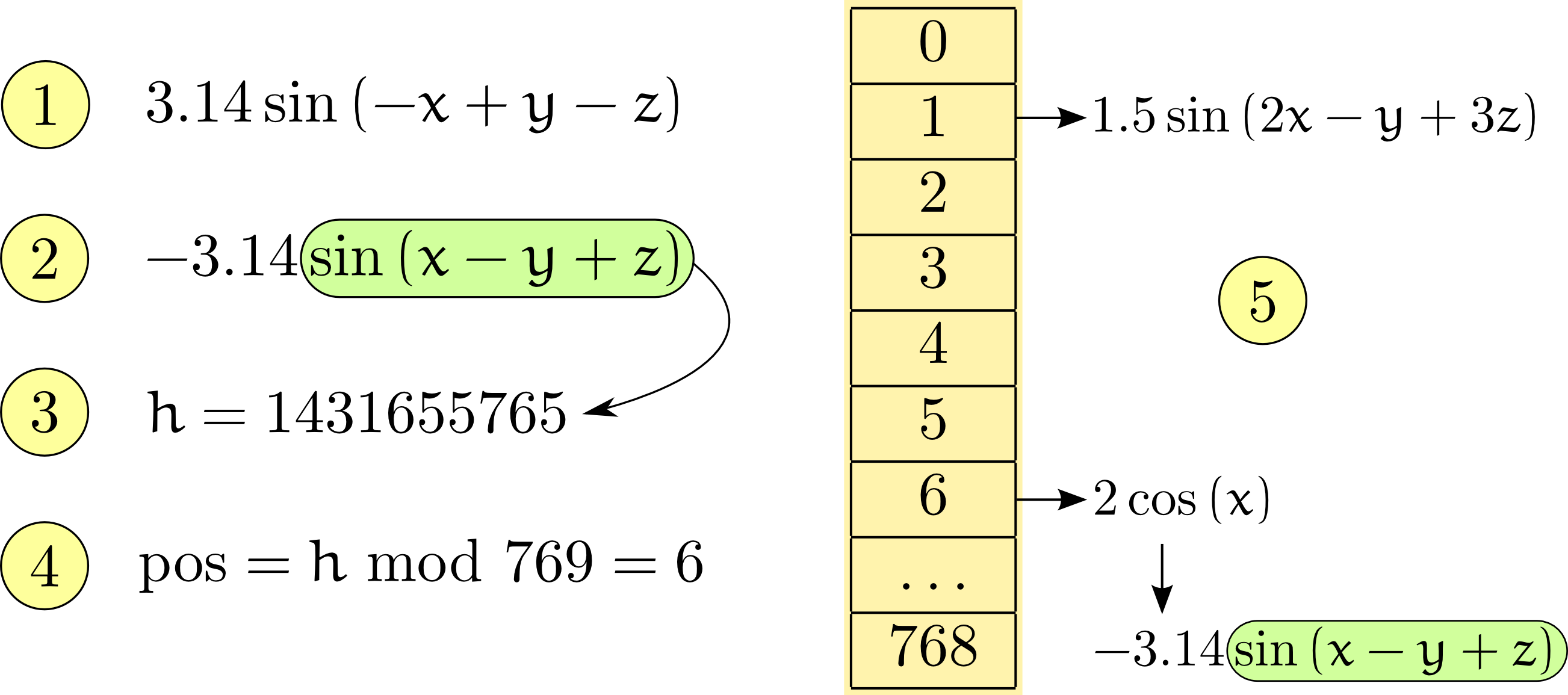
Figure 2: Insertion of a term into a Fourier series. The term (1) is first canonicalised (2), then its hash value, $h$, is calculated from the key (3). The position in the hash table is calculated through the modulo operation (4), which, in this example, produces index number 6. Since the sixth slot of the hash table contains a term with a different key, the term being inserted is then chained in a linked list (5).

5 Series arithmetic

Beside being used frequently in actual computations, arithmetic on series constitutes also the basis of more advanced manipulations (such as the series expansions described in §6). An efficient implementation of basic arithmetic is then a fundamental component of an efficient specialised manipulator.

The sets of series types encountered in Celestial Mechanics typically constitute Abelian groups under the operations of addition and subtraction whose identity elements are series with zero terms. Additionally, such sets are closed under the operation of multiplication, but, in general, it will not possible to express inverse series within a given set in finite terms. In the context of Celestial Mechanics, an effective way to compute real powers (and hence also the inversion) of certain families of series is the generalised binomial theorem, as described in §6.

5.1 Addition and subtraction

The adoption of hashing techniques, as described in §4, allows for a straightforward implementation of the operations of series addition and subtraction. To add a series $S_{2}$ to a series $S_{1}$, it will be enough to simply insert() all terms belonging to $S_{2}$ into $S_{1}$. As described earlier, the insertion routine will take care of dealing with equivalent terms; in case of a subtraction, the terms’ signs will be changed before insertion.

Since hash tables feature expected $\operatorname{O}\!\left(1\right)$ complexity for element insertion, series addition and subtraction will feature expected $\operatorname{O}\!\left(n\right)$ complexity, where $n$ is the number of terms of the series being added or subtracted.

5.2 Multiplication

Series multiplication is the most time-consuming among the basic operations that can be performed on series, and hence an obvious target for heavy optimisation. Generally speaking, to multiply two series $S_{1}$ and $S_{2}$ consisting of $n_{1}$ and $n_{2}$ terms respectively, it will be necessary to multiply each term of $S_{1}$ by each term of $S_{2}$. It follows then that it will be needed to perform $n_{1}n_{2}$ term-by-term multiplications and insertions into the resulting series. The complexity of series multiplication is hence quadratic, or $\operatorname{O}\!\left(n^{2}\right)$, with respect to term-by-term multiplications and insertion operations.

We recall here that polynomials can be multiplied by using asymptotically-faster algorithms, like Karatsuba ([34]) and FFT algorithms ([8]). Such algorithms however are not usually employed in Celestial Mechanics for the following reasons:

• they work best on the assumption that the polynomials to be multiplied are dense ([20]). This is not generally the case in Celestial Mechanics;

• these algortihms are practically faster than $\operatorname{O}\!\left(n^{2}\right)$ multiplication for polynomial degrees that are too high to be encountered in typical Celestial Mechanics problems.

We are not currently aware of algebraic manipulators specialised for Celestial Mechanics using fast polynomial multiplication algorithms.

We can implement multiplication similiarly to addition and subtraction, i.e., by performing term-by-term multiplications and accumulating the results into a newly-created series using the insert() method. Indeed, that’s precisely what happens in Piranha for series in nonzero echelon levels, i.e., when dealing with coefficient series. In such cases the time needed for term-by-term multiplication dwarfs the time needed for term insertion, so it is of little benefit to optimise the performance of term accumulation.

Echelon-0 series, however, feature numerical coefficients, and hence the cost of term multiplication might become comparable to or greater than the cost of term insertion (especially with double-precision coefficients). In this situation the cost of memory allocations and the poor spatial locality exhibited by hash tables employing separate chaining can become performance bottlenecks. For this reason in Piranha we adopt an intermediate representation for the multiplication of suitable echelon-0 series based on an procedure that we conceived autonomously, before learning that it is essentially an application of a known algorithm named Kronecker substitution ([36], [41]).

5.2.1 Kronecker substitution

Kronecker substitution can be intuitively understood in the case of multivariate polynomials with the aid of a simple table laying out the monomials in lexicographic order. The lexicographic representation for three variables $x$, $y$ and $z$, and up to the third power in each variable is displayed in Table 1.

$z$	$y$	$x$	Code
0	0	0	0
0	0	1	1
0	0	2	2
0	0	3	3
0	1	0	4
0	1	1	5
0	1	2	6
0	1	3	7
0	2	0	8
$\ldots$	$\ldots$	$\ldots$	$\ldots$
3	3	3	63

Table 1: Kronecker substitution for a 3-variate polynomial up to the third power in each variable.

The column of codes is obtained by a simple enumeration of the exponents’ multiindices. It can be noted how in certain cases the addition of multiindices (and hence the multiplication of the corresponding monomials) maps to the addition of their codified representation. For instance:

$$c\left(\left[0,0,3\right]\right)+c\left(\left[0,1,0\right]\right)=3+4=7=c\left(\left[0,1,3\right]\right)=c\left(\left[0,0,3\right]+\left[0,1,0\right]\right),$$ (11)

where we have noted with $c=c\left(\mathbf{M}\right)$ the function that codifies a multiindex vector $\mathbf{M}$. An inspection of Table 1 promptly suggests that for an $m$-variate polynomial up to the $n$-th power, $c$’s effect is equivalent to a scalar product between the multiindices vectors and a constant coding vector $\mathbf{c}$ defined as

$$\mathbf{c}=\left[\left(n+1\right)^{m-1},\left(n+1\right)^{m-2},\ldots,n+1,1\right],$$ (12)

so that eq. (11) can be generalised as

$$\mathbf{c}\cdot\left(\mathbf{M}_{1}+\mathbf{M}_{2}\right)=\mathbf{c}\cdot\mathbf{M}_{1}+\mathbf{c}\cdot\mathbf{M}_{2}.$$ (13)

While this equation is valid in general due to the distributivity of scalar multiplication, the codification of a single multiindex will produce a unique code only if the multiindex is representable within the representation defined by $\mathbf{c}$. For the codification represented in Table 1, for instance, we have

$$\mathbf{c}=\left[\left(3+1\right)^{2},3+1,1\right]=\left[16,4,1\right].$$ (14)

If we try to code a monomial in which at least one of the exponents is greater than 3 using eq. (14), we can see how the mapping between multiindices and codes is not univocal any more. For instance the following different multiindices will produce the same code:

$$\left[0,0,4\right]\cdot\left[16,4,1\right] = 4,$$ (15)

$$\left[0,1,0\right]\cdot\left[16,4,1\right] = 4.$$ (16)

Kronecker substitution constitutes an addition preserving homomorphism between the space of integer vectors whose elements are bound in a range and a subset of integers. It is equivalent to considering the elements of the multiindex as the digits of a number in base $n+1$, and transforming it into its decimal counterpart. In the 3-variate example above, for instance, the last row of the table, 333, is decimal 63 in base 4. It also provides a method to reduce multivariate polynomials into univariate ones, as the codes can be seen as exponents of a univariate polynomial.

In Piranha we have adopted a generalisation of Kronecker substitution in which

• we consider variable codification, i.e., each element of the multiindex has its own range of variability,

• we extend the validity of the codification to negative integers and subtraction operations.

The first generalisation allows to compact the range of the codes. If, for instance, the exponent of variable $x$ in the example above varies only from 0 to 1 (instead of varying from 0 to 3 like for $y$ and $z$), we can avoid codes that we know in advance will be associated to nonexisting monomials (i.e., all those in which $x$’s exponent is either 2 or 3). The second generalisation, which derives from the fact that under an appropriate coding vector it is possible to change $\mathbf{M}_{2}$’s sign in eq. (13) retaining the validity of the homomorphism, allows to apply Kronecker substitution to the multiplication of Fourier series. Fourier series multiplication, indeed, requires the ability not only to add but also to subtract the vectors of trigonometric multipliers according to the elementary trigonometric formulas

$$\begin{gathered}A\cos\alpha\cdot B\cos\beta=\frac{AB}{2}\cos\left(\alpha-\beta\right)+\frac{AB}{2}\cos\left(\alpha+\beta\right),\\ A\cos\alpha\cdot B\sin\beta=\frac{AB}{2}\sin\left(\alpha+\beta\right)-\frac{AB}{2}\sin\left(\alpha-\beta\right),\\ A\sin\alpha\cdot B\cos\beta=\frac{AB}{2}\sin\left(\alpha-\beta\right)+\frac{AB}{2}\sin\left(\alpha+\beta\right),\\ A\sin\alpha\cdot B\sin\beta=\frac{AB}{2}\cos\left(\alpha-\beta\right)-\frac{AB}{2}\cos\left(\alpha+\beta\right).\end{gathered}$$ (17)

As far as we have been able to verify, we have not found any indication of previous uses of Kronecker substitution to perform multiplication of Fourier series.

Table 2 shows the generalised Kronecker substitution for a multivariate polynomial (or Fourier series) in which the exponents (or trigonometric multipliers) vary on different ranges.

$x_{m-1}$	$\ldots$	$x_{1}$	$x_{0}$	Code
$e_{m-1,\min}$	$\ldots$	$e_{1,\min}$	$e_{0,\min}$	$0$
$e_{m-1,\min}$	$\ldots$	$e_{1,\min}$	$1+e_{0,\min}$	$1$
$\ldots$	$\ldots$	$\ldots$	$\ldots$	$\ldots$
$e_{m-1,\min}$	$\ldots$	$e_{1,\min}$	$e_{0,\max}$	$e_{0,\max}-e_{0,\min}$
$e_{m-1,\min}$	$\ldots$	$1+e_{1,\min}$	$e_{0,\min}$	$1+e_{0,\max}-e_{0,\min}$
$e_{m-1,\min}$	$\ldots$	$1+e_{1,\min}$	$1+e_{0,\min}$	$2+e_{0,\max}-e_{0,\min}$
$e_{m-1,\min}$	$\ldots$	$1+e_{1,\min}$	$2+e_{0,\min}$	$3+e_{0,\max}-e_{0,\min}$
$\ldots$	$\ldots$	$\ldots$	$\ldots$	$\ldots$

Table 2: Generalised Kronecker substitution for an $m$-variate polynomial (or Fourier series) in which each exponent (or trigonometric multiplier) varies on a different range.

If we define

$$\mathbf{e} = \left(e_{0},e_{1},\ldots,e_{m-1}\right),$$ (18)

$$\mathbf{e}_{\min/\max} = \left(e_{0,\min/\max},e_{1,\min/\max},\ldots,e_{m-1,\min/\max}\right),$$ (19)

$$c_{k} = 1+e_{k,\max}-e_{k,\min},$$ (20)

$$\mathbf{c} = \left(1,c_{0},c_{0}c_{1},c_{0}c_{1}c_{2},\ldots,\Pi_{k=0}^{m-2}c_{k}\right),$$ (21)

$$\chi = \mathbf{c}\cdot\mathbf{e}_{\min},$$ (22)

it is easy to show that the code of the generic multiindex $\mathbf{e}$ is obtained by

$$c\left(\mathbf{e}\right)=\mathbf{c}\cdot\mathbf{e}-\chi.$$ (23)

Codifying monomials and trigonometric keys into integers using Kronecker substitution yields some advantages. First, just like in traditional integer packing techniques, we can save space by using a single integer to represent many integers. Second, we can map both multiindex addition and subtraction to the corresponding operation on a single integer. Finally, in the context of hashing techniques, the codes obtained through Kronecker substitution constitute perfect hash values, in the sense that the mapping between the multiindices and the corresponding codes is univocal. Then, depending on the range of the codes and on the characteristics of the input series, we can adopt two strategies to perform term accumulation during series multiplication:

1. perfect hashing: if there is enough memory available and the input series are not much too sparse, then it is convenient to use the codes of the resulting terms directly as indices in an array (i.e., in a perfect hash table). In this way to accumulate series terms during multiplication it will be enough to multiply term-by-term the coefficients, add/subtract the codes and write directly in the memory address indicated by the newly-generated code;

2. sparse hashing: if the input series are much too sparse or there is not enough memory, then the resulting codes can be reduced through the modulo operation to a smaller value and used to place the terms resulting from the multiplication in a standard (i.e., non-perfect) hash table.

Both these algorithms are discussed in greater detail in §5.2.2.

In order for Kronecker substitution to be effective, it is necessary that the codes vary within a range representable with hardware integers, otherwise the speed benefits related to the codification are reduced. On modern 64 bits architectures, this restriction is seldom limiting in the context of Celestial Mechanics. The monomials of a 6-variate polynomial, for instance, can be codified with Kronecker substitution into 64 bits unsigned integers up to exponent 1624 in all variables. In any case, if Kronecker substitution is not feasible, Piranha will revert to the algorithm, described above, used for nonzero echelon level series.

The main disadvantage of using Kronecker substitution is the need to decode the resulting series. Depending on the density of the input series, the time needed to perform this step can become a relevant fraction of the total time needed for series multiplication.

5.2.2 Cache-friendly perfect and sparse hashing on codified series

Both the perfect and sparse hash algorithms mentioned above perform the following steps:

1. code the input series into vectors of nonzero coefficient-code pairs using Kronecker substitution;

2. multiply coefficient by coefficient the two series, using the addition (and subtraction, for Fourier series) of codes to establish the placement of each resulting coefficient in an appropriate data structure;

3. decode the result into the input series type.

In the case of perfect hashing, the data structure used to store the result of coded series multiplication is a simple array of coefficients. The index of each coefficient resulting from each term-by-term multiplication will simply be given by its corresponding code, resulting from the addition or subtraction of the input codes. In perfect hashing, hence, each term-by-term multiplication consists of a coefficient multiplication, one or two integer additions and one or two memory redirections.

We have to resort to sparse hashing when we cannot use an array to store the resulting coefficients, because an array would be either too large to fit in the available memory or too costly to allocate and setup because of the high sparseness of the input series (which usually translates in high sparseness also for the resulting series). Thus, for sparse hashing we have implemented a cache-friendly hash table for the storage of coefficient-code pairs that minimises memory allocations and tries to maximise spatial locality of reference. Although different in implementation, the logic of term lookup and insertion is the same as explained in Figure 2. Our implementation is essentially a hash table employing separate chaining in which the buckets have fixed sizes and are laid out contiguously in a single dynamically-allocated memory area. In such a structure a rehash is triggered not when the load factor reaches a certain threshold (as it usually happens in standard hash table implementations) but when a bucket is completely filled up. To reduce the need for rehashing, a number of buckets is used as an overflow area to store coefficient-code pairs belonging to filled-up buckets, so that the rehash is dealyed until the overflow buckets are exhausted. The overflow buckets must be checked at every lookup operation. According to our tests, this hash table variant with a bucket depth of 12 is usually filled up to $\sim 30\%$ before needing a rehash.

The design of the hash table used for sparse hashing aims at maximising performance by utilising efficiently the cache memory found on modern computer architectures. The buckets, for instance, consist of arrays instead of linked lists (as commonly implemented in separate chaining) in order to improve spatial locality of reference, so that the load of the first element of the bucket from the slow RAM into the fast cache memory entails also the loading of a number of successive elements. If a linked list were used instead, such prefetching of successive elements would not be possible since in linked lists the second and successive elements are generally not contiguous to the first one; buckets implemented as linked lists hence require a load operation from RAM for every element.

We adopted two other techniques in order to optimise cache memory utilisation for both perfect and sparse hashing:

1. ordering of coded input series: in both algorithms the codes resulting from Kronecker substitution are used to calculate a memory address (they are used directly as an index in perfect hashing, while in sparse hashing they are used as an index after the application of the modulo operation). If we order the coded input series according to the code and we proceed to term-by-term multiplications in two nested for cycles, it follows naturally that in each innermost for cycle (i.e., while iterating over the terms of the second series having fixed a term in the first one) we are going to write into successive memory areas. Doing this both improves prefetching and helps the cache subsystem determine a predictable memory access pattern. According to our tests, this optimisation allowed for a reduction in the time needed to multiply large series up to 40% with respect to the case in which the input series are unordered;

2. cache blocking: another way to optimise cache memory utilisation is to promote temporal locality, i.e., making sure that data is used as often as possible in order to avoid eviction from cache memory. This effect can be obtained through blocking techniques: during series multiplication, instead of fixing a term in the first series and iterating over all the terms of the second series we iterate just over a portion of the second series, then moving on to the second term of the first series and repeating the procedure. In other words, we divide the series in blocks and multiply block-by-block. This ensures that we are going to read and write the same memory areas very frequently, thus maximising the permanence in cache memory. In our tests this optimisation can lead to substantial speed gains: in the case of large polynomials the reduction of the time needed to perform multiplications can reach 70%.

The version of Piranha benchmarked in §8 employs the optimisation techniques described in this section.

6 Nontrivial operations on series

In Celestial Mechanics it is common to encounter algebraic expressions that cannot be mapped directly to Poisson series or polynomials. An expression often arising is, for instance, the square root

$$\sqrt{1-e^{2}},$$ (24)

where $e$ is an orbital eccentricity. In other cases it may be necessary to compute the sine or cosine of a Poisson series.

Such occurrences are usually dealt with through series expansions. Expression (24) may be rewritten in terms of the MacLaurin development

$$\sum_{n=0}^{\infty}\frac{\left(2n\right)!}{\left(1-2n\right)n!^{2}4^{n}}e^{2n}$$ (25)

for $\left|e\right|<1$. Such an expansion truncated to a finite order is often appropriate since in most practical problems of perturbation theory the value of $e$ is small. In Piranha we provide two general series expansions that can be useful to reduce to a representable algebraic form many common occurrencies of problematic expressions.

The first series expansion is employed to compute the real power of a series and uses the generalised binomial theorem ([3]):

$$\left(x+y\right)^{r}=\sum_{k=0}^{\infty}{r\choose k}x^{r-k}y^{k},$$ (26)

where, for our purposes, $r\in\Re$ and $x$ and $y$ are complex numbers. In Piranha the real power of a series $S$ is rewritten in terms of a leading term $L$ and a tail series $T$, so that

$$\left(S\right)^{r} = \left(L+T\right)^{r}$$ (27)

$$= \sum_{k=0}^{\infty}{r\choose k}L^{r-k}T^{k}.$$ (28)

It is the responsibility of the user to make sure that the series is convergent (i.e., $r$ is a positive integer or $\left|L\right|>\left|T\right|$). Piranha will choose the leading term adopting series-specific criterions: for Poisson series and polynomials, for instance, the leading term is the one with lowest total degree, while for Fourier series the leading term is the one with the highest coefficient in absolute value. It is worth noting that while $T$ is subject only to trivially-implementable natural powers, $L$ must be in general amenable to real exponentiation. In case of Poisson series, the real power of the leading term $L$ involves the calculation of the real power of its polynomial coefficient, so that the binomial expansion may be called again to compute $L^{r-k}$ in a somewhat recursive fashion. This method of calculation of real powers can be succesfully applied to expressions such as (24) (effectively producing the same expression as (25)) or to compute the inverse of a suitable series.

The other series expansion implemented in Piranha is used to compute the complex exponential of real Poisson and Fourier series, and it is based upon the Jacobi-Anger expansion ([55]):

$$\exp\left[\imath x\cos\theta\right]=\sum_{n=-\infty}^{\infty}\imath^{n}J_{n}\left(x\right)\exp\left[\imath n\theta\right],$$ (29)

where $J_{n}\left(x\right)$ is the Bessel function of the first kind of integer order $n$, which can be expressed by the MacLaurin development

$$J_{n}(x)=\sum_{l=0}^{\infty}\frac{(-1)^{l}}{2^{2l+n}l!(n+l)!}x^{2l+n}.$$ (30)

By using eq. (29) and eq. (30), and by remembering the property of Bessel functions

$$J_{-n}\left(x\right)=\left(-1\right)^{n}J_{n}\left(x\right),$$ (31)

it is possible to transform the complex exponential of a Poisson series into a product of Poisson series. From the complex exponential, the cosine and sine of the Poisson series can be extracted as the real and imaginary parts respectively. As far as we were able to verify in the literature, no other manipulator implements circular functions of Poisson series using the Jacobi-Anger expansion. Usually such calculations are performed by decomposing the Poisson series into a leading term and a tail (similarly to what is done in the binomial expansion) and by expanding the function through elementary trigonometric formulas:

$$\cos S = \cos\left(L+T\right)$$ (32)

$$= \cos L\cos T-\sin L\sin T.$$ (33)

At this point $\cos T$ and $\sin T$ are expressed through truncated MacLaurin series. Another approach, recently proposed in [38] and based on a Richardson-type elimination scheme, has been shown to be advantageous in certain cases with respect to Taylor expansions both in terms of accuracy and computing time.

With the ability to compute real exponentiation and circular functions on series, it is possible to implement an array of capabilities consisting of special functions and series expansions relevant to Celestial Mechanics applications (thus implementing the basis of what is sometimes called a keplerian processor - see [9] and [11]). Piranha currently implements Bessel functions of the first kind, Legendre polynomials, associated Legendre functions, (rotated) spherical harmonics and the elliptic expansions for $\frac{r}{a}$, $\frac{a}{r}$, $E$, $f$, $\begin{array}[]{c}\cos\\ \sin\end{array}\left(f\right)$ and $\exp\left[\imath nE\right]$ (as seen in standard Celestial Mechanics textbooks, such as [42], Chapter 2).

7 Python bindings

Piranha’s core is a C++ library that can be used within any C++ program. Although we have tried to make the use of the library as friendly as possible (e.g., by using operator overloading), usage as a C++ library remains somehow uncomfortable: a basic knowledge of the C++ programming language is required, and every change of the source code in the main routine must be followed by a recompilation of the whole program, a task that can become slow and cumbersome in the case of generically-programmed libraries like Piranha. Additionally, direct usage as a C++ library is not interactive.

For these reasons we provide a set of Python bindings (called Pyranha) which is intended to be the preferred way of interacting with the manipulator for end-users. In Pyranha, Piranha’s C++ classes are exposed as Python objects with the help of the Boost.Python library. It is important to stress that this is not a translation of C++ code into Python: even as Python objects, Piranha’s classes are still compiled C++ code, so that there is no performance penalty in using the manipulator from Python.

Using Piranha from an interpreted language like Python has several advantages. In our opinion, two important ones are the following:

1. Python ([45]) is an open-source and widely used language, with a standardised syntax, an easy learning curve and a vast amount of publicly-available additional modules;

2. Python can be used interactively. Through enhanced Python shells and graphics libraries it is possible to provide an interactive environment with graphical capabilities. Pyranha takes advantage of the features provided by the IPython shell and the matplotlib graphic library ([28, 39]).

Among Python’s features, of particular relevance for Pyranha are lambda functions, which allow to define small functions inline directly when they are called. Lambda functions are particularly handy for two useful series methods available in Pyranha. The first one is a plotting method, which works in conjunction with the matplotlib module. This method takes as parameter a function that specifies what to plot. The following Python code snippet uses a lambda function to specify that it is being requested to plot the norms of the coefficients of the series foo:

⬇

foo.plot(key = lambda t: t.cf.norm)

This means that from every term t of the series, the coefficient’s norm is extracted and plotted. Another useful method is the filter() method, which is modelled after Python’s builtin function with the same name. filter() is used to extract from series terms satisfying a criterion specified through a lambda function:

⬇

foo.filter(lambda t: t.key.freq > 0)

In this case we are extracting all terms of a Poisson/Fourier series whose frequency (which is a property of the trigonometric key) is positive. filter() can work in a recursive fashion in case of nonzero echelon level series. This means that it is possible to pass more than one argument: the first argument is used to filter the terms of the series, the second argument to filter the terms of each coefficient series in the terms surviving from the first filtering, and so on. filter() can be useful in perturbation theories, when it is necessary to select the terms of the series which are relevant to the physical problem that is being solved.

8 Benchmarks

In this section we present a few benchmarks on the multiplication of echelon-0 series. The systems benchmarked are: SDMP, a library for sparse polynomial multiplication and division ([40]), TRIP, an algebraic manipulator devoted to Celestial Mechanics ([23]), Pari, a computer algebra system for number theory ([44]), Magma ([6]), Singular ([24]) and Maple. The usual caveats about benchmarking as a method to measure performance apply. Additionally, we must preface the following disclaimers:

• measurements for other systems were taken by SDMP co-author Roman Pearce on a Linux server equipped with a Core2 Xeon 3.0 GHz CPU with 4MB of L2 cache, while Piranha’s measurements were taken on a Linux laptop equipped with a Core2 1.8 GHz CPU with 2MB of L2 cache (the GCC compiler version 4.3.2 was used to compile Piranha). We have chosen to express the results as both the original timings in seconds and clock cycles per term-by-term multiplication (ccpm) in an effort to provide a uniform scale. It must be noted however that the latter unit of measure fails to give meaningful results when the computation time is bounded by memory transfers (i.e., when most of the time is spent loading data from RAM). In such cases the speed of execution of the same task will depend more on the speed of the memory subsystem than on the CPU speed;

• we have chosen to express Piranha’s results as sums of two numbers: the first number measures the speed of the actual multiplication, while the second number represents the time spent unpacking the result from the coded series representation back into the standard series representation (as explained at the beginning of §5.2.2). The reason for this distinction will be explained in the comments about the individual benchmarks;

• the computer algebra systems tested adopt different representations for coefficients and exponents (or trigonometric multipliers), so the relevance of these benchmarks is related to the adequacy of the representations used in the various systems with respect to the task at hand. Additionally, there are differences also in the representation of series (certain systems, such as Pari and TRIP for instance, use a recursive representation for polynomials, while SDMP’s and Piranha’s representations are distributed).

We would like to gratefully thank Roman Pearce for allowing us to reproduce the benchmarks he performed. The original benchmarks are available online at the following address:

http://www.cecm.sfu.ca/~rpearcea/

8.1 Fateman’s benchmark

The first benchmark is modelled after that proposed by Richard Fateman in [20], and consists of the calculation of

$$s\left(s+1\right),$$ (34)

where $s$ is defined as the multivariate polynomial

$$s=\left(1+x+y+z+t\right)^{30}.$$ (35)

The computation is expressed as $s\left(s+1\right)$ instead of, e.g., $s^{2}+s$, to prevent “smart” computer algebra systems to calculate $s^{2}$ more efficiently than through a multiplication (e.g., by multinomial expansion). $s$ and $s+1$ consist of $46\,376$ terms, while the resulting polynomial consists of $635\,376$ terms. The results are displayed in Table 3. Some necessary remarks:

System	Timings (seconds, ccpm)
Piranha 2008.11 (double-precision)	5.4 + 0.6, 4.5 + 0.5
SDMP September 2008 (monomial = 1 word)	47, 65
TRIP v0.99 (double-precision)	44, 61
Pari 2.3.3 (w/ GMP)	512, 714
Magma V2.14-7	679, 947
Singular 3-0-4	1482, 2067
Maple 11	15986, 22298

Table 3: Timings for Fateman’s benchmark.

• the densities of the input polynomials are high enough to make the perfect hashing algorithm viable;

• double-precision coefficients, used by Piranha and TRIP, do not allow to represent exactly the coefficients of the resulting polynomial;

• SDMP uses inline assembly for the multiplication of 61 bits input integer coefficients into 128 bits integer coefficients. On Core2 CPUs, this is expected to cost around 4 times the cost of double-precision multiplication;

• other systems use arbitrary-precision coefficients.

In the case of manipulators devoted to Celestial Mechanics, this test represents more of a limit case than a computation likely to be encountered in actual applications.

In the case of Piranha’s timing we remark that, since double-precision multiplication on Core2 CPUs costs around 4 clock cycles when working in cache, the use of the perfect hashing algorithm allows to approach the theoretical speed limit for this kind of computation performed with classical algorithms. When disabling the cache optimisations described in §5.2.2 the running time for this benchmark is around 36 seconds. We also note how the time needed to unpack the resulting coded polynomial (0.6 s) is a small fraction of the time needed for the multiplication of the input polynomials. Finally, for comparison we note that if Piranha is benchmarked using multiprecision GMP integer coefficients, the running time for this benchmark becomes 90 s (or 75 ccpm).

8.2 Sparse polynomial multiplication benchmark

This benchmark was proposed originally by Michael Monagan and Roman Pearce, and consists of the following polynomial multiplication:

$$\left(1+x+y+2z^{2}+3t^{3}+5u^{5}\right)^{12}\cdot\left(1+u+t+2z^{2}+3y^{3}+5x^{5}\right)^{12}.$$ (36)

Since the polynomials being multiplied consist of $6\,188$ terms each and the result consists of $5\,821\,335$ terms, this multiplication is much more sparse than the one featured in the previous benchmark. For Piranha this means that the perfect hashing algorithm is not viable and that sparse hashing must be employed instead. The results are displayed in Table 4.

System	Timings (seconds, ccpm)
Piranha 2008.11 (double-precision)	3 + 6.8, 141 + 319
SDMP September 2008 (monomial = 1 word)	1.5, 121
TRIP v0.99 (double-precision)	1.9, 148
Pari 2.3.3 (w/ GMP)	54, 4231
Magma V2.14-7	24, 1880
Singular 3-0-4	59, 4622
Maple 11	333, 26089

Table 4: Timings for sparse polynomial multiplication.

The most interesting remark for Piranha is the time spent unpacking the coded series back into the standard series representation, which amounts to more than twice the time spent for the actual multiplication. This behaviour is the combined effect of the following causes:

• we are using a hash table with standard semantics, which means that each insertion function will result in a lookup of the term. This lookup is not necessary because we know that by construction the resulting coded series features unique terms. By implementing a custom hash table with an alternative unchecked insertion function we could avoid pointless term comparisons;

• to decode the coded series we need to apply repeatedly costly integer divisions and modulo operations, which are particularly cumbersome in this benchmark given the high ratio between the number of term-by-term multiplications and the size of the resulting polynomial. For this specific benchmark we could avoid codification altogether since there are no negative exponents and the exponents’ values are bounded in the $\left[0,120\right]$ interval. It follows then that in this case we could simply pack the exponents as, e.g., 8 bits integers into a 64 bits word and obtain the same efficiency as Kronecker substitution, without the need to apply division and modulo operations for the decodification. This optimisation will be implemented in a future version of Piranha;

• the hash_set data structure needs to perform many memory allocations. While this issue can be mitigated by using a pool memory allocator, this solution does not avoid frequent cache-unfriendly memory accesses.

As a test, we have tried to see what happens if, instead of unpacking the series into a hash_set, we simply copy the codes into a plain array. This approach is similar to that adopted by some manipulators which employ plain array-like storage methodologies. The result is that the total running time is reduced to 3.2 s, or 150 ccpm. Although this approach would allow to consistently increase performance, for the time being we are oriented towards maintaining the current implementation. In addition to the fact that it is possible to improve performance with the techniques described above (hash table implementation with additional insertion semantics, avoiding needless encoding, pool memory allocator), the current programming model is in our opinion convenient and clear and allows for capabilities, such as comparison of series in linear time and identification of terms in constant time, which have proven to be useful in practice.

8.3 Fourier series multiplication

This benchmarks consists of the squaring of the ELP3 Fourier series representing the solution of the main problem of the lunar theory for the Moon’s distance in the ELP2000 theory ([14]). The ELP3 series consists of 702 terms and the squaring produces a series with $11\,673$ terms. The squaring is performed 20 times in order to minimise the effect of the time needed to load the series from file. The sparseness of the ELP3 Fourier series, despite higher than in Fateman’s benchmark, is still low enough to make the perfect hashing algorithm viable.

We report in Table 5 the timings for Piranha and TRIP. We report just the plain timings because TRIP’s results, communicated to us by TRIP’s co-author Mickaël Gastineau, were taken on a CPU which is slower than the Core2 CPU used for Piranha and whose characteristics we are not aware of. According to our tests, the Core2 CPU should be $\sim 1.5$ times faster.

System	Timings (seconds)
Piranha 2008.11 (double-precision)	0.495
TRIP v0.99 (double-precision)	1.352

Table 5: Timings for Fourier series multiplication benchmark.

In Piranha’s case the timings translate in roughly 90 clock cycles per term-by-term multiplication. It is then evident that here the overhead of decoding the coded series is dominating, as the multiplication of Fourier series terms consists of a double-precision multiplication ($\sim 4$ clock cycles) and a double-precision division ($\gtrsim 6$ clock cycles), as per eqs. (17). To confirm this interpretation we have computed first $\textnormal{ELP3}^{2}\cdot\textnormal{ELP3}^{2}$ and then $\textnormal{ELP3}^{4}\cdot\textnormal{ELP3}^{4}$ (where $\textnormal{ELP3}^{4}$ consists of $192\,000$ terms). For these other two benchmarks we measured a total cost of 15 ccpm and 11 ccpm respectively, thus confirming that the cache-optimised perfect hashing algorithm allows to reach a high throughput, especially for long series.

9 Conclusions, future work and availability

In this contribution we have provided an overview of the architecture upon which the Piranha algebraic manipulator is built. We have described the high-level representation of series, the storage method for terms, based on hashing techniques, and the algorithms used during series arithmetic. We have shown how Kronecker substitution can be applied also to the multiplication of Fourier series and how it allows to reach promising performance for series multiplication. We also have briefly described how using Piranha from Python can open up interesting possibilities of interaction with series objects, and how it is possible to develop nontrivial functions of series in practical Celestial Mechanics problems.

Future work on Piranha will target the following areas of interest:

• implementation of echeloned Poisson series;

• implementation of multiprecision floating-point coefficients (possibly through the MPFR library, see [21]);

• implementation of interval arithmetic for both double-precision and multiprecision coefficients;

• enhancements for the keplerian processor and implementation of standard algorithms of perturbation theories in the context of Celestial Mechanics,

• performance improvements for the multiplication of very sparse series (as explained in §8.2);

• parallelisation for the most time-consuming operations;

• enhancements for the Python bindings, in order to improve interactivity, ease of use and flexibility (also by means of graphical user interface elements).

We are also evaluating the possibility to provide some form of interaction between Piranha and general-purpose computer algebra systems. We are particularly interested in the possibility to interact with the open-source mathematics software Sage ([52]).

Piranha is freely available under the terms of the GNU public license, and it can be downloaded from the website

http://piranha.tuxfamily.org

The manipulator runs on Unix and Windows platforms, and it can be compiled with a reasonably recent version of a C++ compiler (the GCC, Intel and Visual Studio compilers have been successfully used so far). We hope to be able to gather enough interest around Piranha to establish a community of users and developers in the future.

10 Acknowledgements

We would like to thank Elena Fantino for proofreading this manuscript and for constant encouragement. We would also like to thank Roman Pearce and Mickaël Gastineau for testing Piranha and for helpful discussion.

References

- [1] A. Abad and J. F. San-Juan, PSPC: a Poisson Series Processor Coded in C, in Dynamics and Astrometry of Natural and Artificial Celestial Bodies, K. Kurzynska, F. Barlier, P. K. Seidelmann, and I. Wyrtrzyszczak, eds., 1994, p. 383.
- [2] Andrei Alexandrescu, Modern C++ design: generic programming and design patterns applied, Addison-Wesley Longman Publishing Co., Inc., Boston, MA, USA, 2001.
- [3] George B. Arfken and Hans J. Weber, Mathematical Methods for Physicists, Academic Press, sixth ed., 2005.
- [4] I. O. Babaev, V. A. Brumberg, N. N. Vasil’Ev, T. V. Ivanova, V. I. Skripnichenko, and S. V. Tarasevich, UPP - Universal system for analytical operations with Poisson series, Astron. i geod., Tomsk, No. 8, p. 49 - 53, 8 (1980), pp. 49–53.
- [5] The Boost C++ Libraries. http://www.boost.org, 2008.
- [6] Wieb Bosma, John Cannon, and Catherine Playoust, The MAGMA algebra system I: the user language, J. Symb. Comput., 24 (1997), pp. 235–265.
- [7] S. R. Bourne and J. R. Horton, The design of the Cambridge algebra system, in SYMSAC ’71: Proceedings of the second ACM symposium on Symbolic and algebraic manipulation, New York, NY, USA, 1971, ACM, pp. 134–143.
- [8] E. Oran Brigham, The fast Fourier transform and its applications, Prentice-Hall, Inc., Upper Saddle River, NJ, USA, 1988.
- [9] Roger A. Broucke, How to Assemble a Keplerian Processor, Celestial Mechanics and Dynamical Astronomy, 2 (1970), p. 9.
- [10] Roger A. Broucke and K. Garthwaite, A programming system for analytical series expansions on a computer, Celestial Mechanics and Dynamical Astronomy, 1 (1969), pp. 271–284.
- [11] V. A. Brumberg, S. V. Tarasevich, and N. N. Vasil’Ev, Specialized Celestial Mechanics Systems for Symbolic Manipulation, Celestial Mechanics, 45 (1989), pp. 149–162.
- [12] Jean Chapront, Colbert: Manipulateur de séries de Fourier à coefficients littéraux. ftp://syrte.obspm.fr/pub/polac/4_programming_tools/2_colbert/colbert.pd%f, 2003.
- [13] , Gregoire: Manipulateur de séries de Poisson à coefficients numériques. ftp://syrte.obspm.fr/pub/polac/4_programming_tools/1_gregoire/gregoire.%pdf, 2003.
- [14] M. Chapront-Touzé and J. Chapront, ELP2000-85: a semianalytical lunar ephemeris adequate for historical times, Astronomy & Astrophysics, 190 (1988), pp. 342–352.
- [15] James O. Coplien, Curiously recurring template patterns, C++ Rep., 7 (1995), pp. 24–27.
- [16] Thomas H. Cormen, Charles E. Leiserson, and Ronald L. Rivest, Introduction to Algorithms, MIT Press/McGraw-Hill, 1990.
- [17] J. M. A. Danby, André Deprit, and A. R. M. Rom, The symbolic manipulation of Poisson series, in SYMSAC ’66: Proceedings of the first ACM symposium on Symbolic and algebraic manipulation, New York, NY, USA, 1966, ACM Press, pp. 0901–0934.
- [18] R. R. Dasenbrock, A FORTRAN-Based Program for Computerized Algebraic Manipulation, Technical Report 8611, Naval Research Laboratory, 1982.
- [19] A. T. Doodson, The harmonic development of the tide generating potential, Proceedings of the Royal Society, 100 (1922), pp. 305–329.
- [20] Richard Fateman, Comparing the speed of programs for sparse polynomial multiplication, SIGSAM Bull., 37 (2003), pp. 4–15.
- [21] Laurent Fousse, Guillaume Hanrot, Vincent Lefèvre, Patrick Pélissier, and Paul Zimmermann, MPFR: A multiple-precision binary floating-point library with correct rounding, ACM Trans. Math. Softw., 33 (2007), p. 13.
- [22] Mickaël Gastineau and Jacques Laskar, Development of TRIP: Fast Sparse Multivariate Polynomial Multiplication Using Burst Tries, in Computational Science - ICCS 2006, Springer Berlin / Heidelberg, 2006, pp. 446–453.
- [23] , TRIP 0.99. http://www.imcce.fr/Equipes/ASD/trip/trip.html, 2008.
- [24] G.M. Greuel, G. Pfister, and H. Schönemann, Singular: a Computer Algebra System for Polynomial Computations. http://www.singular.uni-kl.de, 2007.
- [25] Steffen Heinz, Justin Zobel, and Hugh E. Williams, Burst tries: a fast, efficient data structure for string keys, ACM Trans. Inf. Syst., 20 (2002), pp. 192–223.
- [26] Jacques Henrard, A survey of Poisson series processors, Celestial Mechanics and Dynamical Astronomy, 45 (1988), pp. 245–253.
- [27] Paul Herget and Peter Musen, The calculation of literal expansions, The Astronomical Journal, 64 (1959), p. 11.
- [28] An Enhanced Python Shell. http://ipython.scipy.org, 2008.
- [29] T. V. Ivanova, PSP: A new Poisson series processor, in IAU Symp. 172: Dynamics, Ephemerides, and Astrometry of the Solar System, S. Ferraz-Mello, B. Morando, and J. E. Arlot, eds., 1996, p. 283.
- [30] , A New Echeloned Poisson Series Processor (EPSP), Celestial Mechanics and Dynamical Astronomy, 80 (2001), pp. 167–176.
- [31] III W. H. Jefferys, A FORTRAN-based list processor for Poisson series, Celestial Mechanics and Dynamical Astronomy, 2 (1970), pp. 474–480.
- [32] , A Precompiler for the Formula Manipulation System Trigman, Celestial Mechanics and Dynamical Astronomy, 6 (1972), p. 117.
- [33] Àngel Jorba, A Methodology for the Numerical Computation of Normal Forms, Centre Manifolds and First Integrals of Hamiltonian Systems, Experimental Mathematics, 8 (1999), pp. 155–195.
- [34] A. Karatsuba and Y. Ofman, Multiplication of many-digital numbers by automatic computers, Translation in Physics-Doklady, 7 (1963), pp. 595–596.
- [35] Donald E. Knuth, The Art of Computer Programming, vol. 3: Sorting and Searching, Addison-Wesley, second ed., 1998.
- [36] Leopold Kronecker, Grundzüge einer arithmetischen theorie der algebraischen grössen, Journal Für die reine und angewandte Mathematik, 92 (1882), pp. 1–122.
- [37] E. D. Kuznetsov and K. V. Kholshevnikov, Expansion of the Hamiltonian of the Two-Planetary Problem into the Poisson Series in All Elements: Application of the Poisson Series Processor, Solar System Research, 38 (2004), pp. 147–154.
- [38] M. D. C. Martínez, J. F. Navarro, and J. M. Ferrándiz, An improved algorithm to compute circular functions of Poisson series, Celestial Mechanics and Dynamical Astronomy, 99 (2007), pp. 59–68.
- [39] A Python 2D plotting library. http://matplotlib.sourceforge.net/, 2008.
- [40] Michael Monagan and Roman Pearce, Polynomial Division using Dynamic Arrays, Heaps, and Packed Exponent Vectors, in Springer-Verlag LNCS 4770, 2007, pp. 295–315.
- [41] Robert T. Moenck, Practical fast polynomial multiplication, in SYMSAC ’76: Proceedings of the third ACM symposium on Symbolic and algebraic computation, New York, NY, USA, 1976, ACM, pp. 136–148.
- [42] Carl D. Murray and Stanley F. Dermott, Solar System Dynamics, Cambridge University Press, February 2000.
- [43] Juan Navarro and José Ferrándiz, A New Symbolic Processor for the Earth Rotation Theory, Celestial Mechanics and Dynamical Astronomy, 82 (March 2002), pp. 243–263.
- [44] PARI/GP Development Headquarters. http://pari.math.u-bordeaux.fr/, 2008.
- [45] The Python Programming Language. http://www.python.org, 2008.
- [46] M. V. Ramakrishna and Justin Zobel, Performance in practice of string hashing functions, in Database Systems for Advanced Applications, 1997, pp. 215–224.
- [47] D. L. Richardson, PARSEC: An Interactive Poisson Series Processor for Personal Computing Systems, Celestial Mechanics and Dynamical Astronomy, 45 (1989), p. 267.
- [48] Arnold Rom, Mechanized Algebraic Operations (MaO), Celestial Mechanics and Dynamical Astronomy, 1 (1970), p. 301.
- [49] , Echeloned Series Processor (ESP), Celestial Mechanics, 3 (1971), pp. 331–345.
- [50] F. Roosbeek, RATGP95: a harmonic development of the tide-generating potential using an analytical method, Geophysical Journal International, 126 (1996), pp. 197–204.
- [51] Félix San-Juan and Alberto Abad, Algebraic and symbolic manipulation of Poisson series, Journal of Symbolic Computation, 32 (2001), pp. 565–572.
- [52] William Stein, Sage: Open Source Mathematical Software, The Sage Group, 2008. http://www.sagemath.org.
- [53] D. Stoutemyer, Which Polynomial Representation is Best? Surprises Abound!, in Proceedings of the 1984 Macsyma Users’ Conference, New York, NY, USA, 1984, Schenectady, pp. 221–243.
- [54] Torbjörn Granlund, GNU Multiple Precision Arithmetic Library. http://gmplib.org/, 2008.
- [55] G. N. Watson, A Treatise on the Theory of Bessel Functions, Cambridge Univ. Press, Cambridge, UK, second ed., 1995.