Probing the $d_{x^{2}-y^{2}}$-wave Pomeranchuk instability by ultrasound

Abstract

Selection rules of ultrasound attenuation and sound velocity renormalization are analyzed in view of their potential application to identify Pomeranchuk instabilities (electronic nematic phase). It is shown that the transverse sound attenuation along $[110]$ direction is enhanced by the Fermi surface fluctuations near a $d_{x^{2}-y^{2}}$-wave Pomeranchuk instability, while the attenuation along $[100]$ direction remains unaffected. Moreover the fluctuation regime above the instability is analyzed by means of a self-consistent renormalization scheme. The results could be applied directly to Sr₃Ru₂O₇ which is a potential candidate for a Pomeranchuk instability at its metamagnetic transition in strong magnetic fields.

I Introduction

In 1958, Pomeranchuk Pomeranchuk considered stability conditions for normal isotropic Fermi liquids and argued that, besides a uniform (spin-dependent) deformation of the Fermi surface, i.e., an itinerant ferromagnetic instability, residual quasiparticle interactions can induce a non-uniform deformation of the Fermi surface. Since then, an inhomogeneous deformation of a Fermi surface caused by quasiparticle interactions is frequently referred to as “Pomeranchuk instability (PI)” It is sometimes called “nematic” electron liquid Oganesyan01 because such a Fermi surface deformation can be characterized by a director order parameter which is used to describe a nematic phase in conventional liquid crystals. The nematic order introduces an anisotropy in the otherwise isotropic physical quantities, and the strong anisotropy of the longitudinal resistivity observed in a clean two-dimensional electron system under high magnetic fields was interpreted as a signal of the development of the nematic order. Lilly99

In lattice systems the term PI is commonly used to refer to a Fermi surface deformation which breaks the symmetry of the underlying lattice. In case of two-dimensional square lattices, it was shown Yamase00 ; Halboth ; Hankevych ; Valenzuela that a PI with $d_{x^{2}-y^{2}}$ symmetry can be realized near van Hove fillings, which then reduces the $C_{4}$ symmetry of the original Fermi surface to $C_{2}$ symmetry. These findings have stimulated a number of further theoretical works Honerkamp02 ; Frigeri02 ; Kee03a ; Kee03b ; Metzner03 ; Arne03 ; Yamase04 ; Khavkine ; Kee05 ; Yamase05 ; DellAnna06 ; DellAnna07 ; Jakubczyk08 on the nature of a $d_{x^{2}-y^{2}}$-wave PI. Recently this phase has attracted a renewed interest in several fields of solid state physics. The occurrence of a $d_{x^{2}-y^{2}}$-wave PI is hotly debated as a possible explanation for the curious phase found in the bilayer ruthenate Sr₃Ru₂O₇ under strong magnetic field. Grigera04 ; Borzi07 Also a $d_{x^{2}-y^{2}}$-wave PI may provide an explanation for the anisotropy in the magnetic excitation spectrum observed in cuprate superconductors, Hinkov04 ; Hinkov08 and a similar argument is ongoing in the context of new iron-pnictide superconductors. Xu08 ; Zhai09 An analogous state in the spin channel was also proposed Hirsch90 ; Wu04 ; Wu07 and used to explain the so-called hidden-order phase found in URu₂Si₂ Varma05 .

Despite these extensive discussions, however, an identification of such a $d_{x^{2}-y^{2}}$-wave PI is not an easy task. The problem lies in the difficulty in finding an experimental probe which couples to the order parameter of the $d_{x^{2}-y^{2}}$-wave PI. Unlike a magnetic transition where we can detect the magnetic susceptibility using neutron scattering experiment, it is hard to detect the corresponding susceptibility for a $d_{x^{2}-y^{2}}$-wave PI which occurs in the charge degrees of freedom. In Ref. Doh07, , it was suggested that a spatial pattern of the local density of states provides a direct probe of the $d_{x^{2}-y^{2}}$-wave PI. It is however applicable only through surface probes, a scanning tunneling microscopy, which is easily influenced by surface conditions. Therefore, it is desirable to have another way to identify the $d_{x^{2}-y^{2}}$-wave PI based on the bulk properties of a sample.

From the point of view that the characteristic anisotropy of a $d_{x^{2}-y^{2}}$-wave PI can be easily wiped out in a macroscopic scale by a formation of domains between two degenerate ground states [FIG. 1 (b) and (c)], Grigera04 ; Doh07 it had better concentrate on the fluctuation effects above the transition temperature Emery76 ; Adachi01 rather than concentrate on the phenomena deep inside of the ordered state. The basic idea presented in this paper is that we can use phonons for the detection of the $d_{x^{2}-y^{2}}$-wave PI. This idea is based on the fact that phonons not only have a coupling to the order parameter of a $d_{x^{2}-y^{2}}$-wave PI through electron-phonon interactions, but also have a propagation-direction-selective coupling. By combining this remarkable property of phonons with a well known fact that damping of phonons (sound attenuation) exhibits a remarkable divergence near a second order phase transitions, Landau54 we can pick up information on the $d_{x^{2}-y^{2}}$-wave PI. In other words, the fluctuation sound attenuation caused by a $d_{x^{2}-y^{2}}$-wave PI can be regarded as a direct probe of the unconventional charge susceptibility characterizing this ordered state.

In this paper, we investigate the behavior of the fluctuation enhancement of the sound attenuation caused by a $d_{x^{2}-y^{2}}$-wave PI. For this purpose, we use two different approaches. The first one is a phenomenological argument using a Gaussian Ginzburg-Landau-Wilson action. The second one is a microscopic analysis starting from a quasi-two-dimensional Hubbard model with on-site and nearest-neighbor repulsions, which is supplemented by the self-consistent renormalization (SCR) theory Moriya85 to treat the fluctuation effects. Both approaches are shown to give the same result that there is a selection rule in the fluctuation enhancement of the sound attenuation and sound velocity softening near a $d_{x^{2}-y^{2}}$-wave PI, depending on the propagation directions and polarizations. This leads to a conclusion that we can utilize these properties to detect the $d_{x^{2}-y^{2}}$-wave PI with the aid of ultrasound measurements.

The plan of this paper is as follows. In Sec. II, we present a phenomenological argument to see how the Fermi surface fluctuations near a $d_{x^{2}-y^{2}}$-wave PI manifest themselves in transverse sound attenuation. The main message of this paper is essentially given in this section. In Sec. III, we present a microscopic analysis of a $d_{x^{2}-y^{2}}$-wave PI, and discuss the mean field phase diagram as well as the effects of fluctuations. Besides, we present a microscopic calculation of the fluctuation sound attenuation, which reinforces the result of the phenomenological argument in Sec. II. Finally in Sec. IV, we summarize our result and give a discussion on the application of our result to the bilayer ruthenate Sr₃Ru₂O₇. We use the unit $k_{B}=\hbar=1$ throughout this paper.

II Phenomenological approach

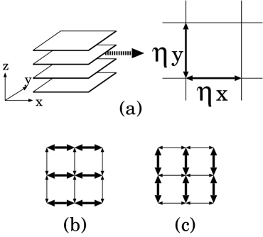
Figure 1: We consider a quasi two-dimensional system composed of a stack of two-dimensional square lattices. The order parameter of a $d_{x^{2}-y^{2}}$-wave PI considered in this work is defined by Eq. (1) where $\eta_{x}$ ($\eta_{y}$) represents the strength of the bond along $x$ ($y$) direction as shown in FIG. 1 (a). The two states in FIG. 1 (b) and (c) are degenerate where the thickness of arrows indicates the strength of the bond.

In this section, we present a phenomenological argument to see how the Fermi surface fluctuations near a $d_{x^{2}-y^{2}}$-wave PI manifest themselves in phonon properties. We pay special attention to the propagation-direction resolved sound attenuation. Because we consider the fluctuation effects above the transition point and mainly focus on the transverse sound attenuation, our argument is essentially different from that given in Ref. Kee03a, where the longitudinal sound propagation below the transition point was discussed.

The order parameter of a $d_{x^{2}-y^{2}}$-wave PI Yamase00 ; Halboth which is considered in this work is defined by [see also Eq. (25)]

$$\eta = \frac{1}{2}\left(\eta_{x}-\eta_{y}\right),$$ (1)

where $\eta_{x}(\eta_{y})$ denote the bond strength along $x$ ($y$) direction (Fig.1) of the underlying square lattice. The order parameter $\eta$ is odd under the permutation $x\leftrightarrow y$. In the presence of nonzero $\eta$, the bond strength along $x$ and $y$ directions are different, hence it deforms the lattice and affects the phonon properties.

Up to the lowest order in $\eta$, the mode-coupling term $\delta F_{\rm GL}$ between lattice (phonon) and the PI order parameter is given by

$$\delta F_{\rm GL}({\bm{U}},\eta) = \kappa\sum_{{\bm{Q}}=({\bm{q}},Q_{z})}\Big{[}u_{xx}({\bm{Q}})-u_{yy}({\bm{Q}})\Big{]}\eta(-{\bm{Q}}),$$ (2)

where ${\bm{Q}}=({\bm{q}},Q_{z})$ is a three-dimensional wavevector with the in-plane component ${\bm{q}}$ and the out-of-plane component $Q_{z}$, $\kappa$ is the coupling constant, $u_{xx}-u_{yy}={\rm i}q_{x}u_{x}-{\rm i}q_{y}u_{y}$ with the lattice displacement field ${\bm{U}}=({\bm{u}},U_{z})$. The above form of the coupling is allowed from the symmetry reason because under the permutation $x\leftrightarrow y$ both $\eta$ and $u_{xx}-u_{yy}$ are odd, keeping the coupling invariant.

We now study how phonons couple to the order parameter of a $d_{x^{2}-y^{2}}$-wave PI depending on their propagation direction and polarization. For the moment, we consider the case where the wavevector and the polarization vector of a sound wave lie within a conducting layer, i.e., ${\bm{Q}}=({\bm{q}},0)$ and ${\bm{U}}=(u_{x},u_{y},0)$, because interesting results come out in this case. Then, the longitudinal (transverse) phonon $u_{L}$ ($u_{T}$) can be written as $u_{L}=\widehat{q}_{x}u_{x}+\widehat{q}_{y}u_{y}$ ($u_{T}=\widehat{q}_{y}u_{x}-\widehat{q}_{x}u_{y}$) with $\widehat{\bm{q}}={\bm{q}}/|{\bm{q}}|$.

Consider a sound wave propagating along $[100]$-direction (i.e., $\widehat{q}_{y}=0$). In this case, using the fact that $u_{xx}-u_{yy}={\rm i}|{\bm{q}}|u_{L}$ when $\widehat{q}_{y}=0$, we can write $\delta F_{\rm GL}$ in Eq. (2) as

$$\delta F_{\rm GL}({\bm{u}},\eta) = \kappa\sum_{{\bm{q}}}\Big{(}{\rm i}|{\bm{q}}|u_{L}({\bm{q}})\Big{)}\eta(-{\bm{q}}).$$ (3)

On the other hand, when a sound wave is propagating along $[110]$-direction (i.e., $\widehat{q}_{x}=\widehat{q}_{y}$), the mode-coupling term (2) can be written as

$$\delta F_{\rm GL}({\bm{u}},\eta) = \kappa\sum_{{\bm{q}}}\Big{(}{\rm i}|{\bm{q}}|u_{T}({\bm{q}})\Big{)}\eta(-{\bm{q}}).$$ (4)

Equations (3) and (4) mean that, through the interaction (2), the longitudinal phonons couple to the $d_{x^{2}-y^{2}}$-wave PI only when they have their wavevector along [100]-direction, while transverse phonons does only when they have their wavevector along [110]-direction.

Using these results [Eqs. (3) and (4)], we next study the effect of the fluctuations of $\eta$ on sound attenuation. Dynamical behaviors of sounds are described by the following action for phonons, Kleinert

$$S_{\rm ph}({\bm{u}}) = \frac{\rho_{\rm ion}}{2}\sum_{{\bm{q}},\omega_{m}}\Big{(}u_{L}^{*}({\bm{q}},\omega_{m}){K}_{L}({\bm{q}},{\rm i}\omega_{m})u_{L}({\bm{q}},\omega_{m})$$ (5)

$$+\;{u}^{*}_{T}({\bm{q}},\omega_{m}){K}_{T}({\bm{q}},{\rm i}\omega_{m}){u}_{T}({\bm{q}},\omega_{m})\Big{)},$$

where the unrenormalized kernel has the form ${K}^{(0)}_{\nu}({\bm{q}},{\rm i}\omega_{m})=\omega_{m}^{2}+(s^{(0)}_{\nu})^{2}\;q^{2}$ with $\nu$ being the polarization index $L$ or $T$. Here, $s^{(0)}_{L}$ and $s^{(0)}_{T}$ the bare longitudinal and transverse sound velocities, $\rho_{\rm ion}$ the mass density of ions, and $\omega_{m}=2\pi Tm$ is the bosonic Matsubara frequency. The information on phonon dynamics is extracted by studying the retarded quantity $K^{R}_{\nu}({\bm{q}},\omega)=K_{\nu}({\bm{q}},{\rm i}\omega_{m}\to\omega+{\rm i}0_{+})$. In the presence of itinerant electrons, excitations of particle-hole pairs yield an imaginary part in $K^{R}_{\nu}$ of the form AGD ${\rm Im}K^{R}_{\nu}({\bm{q}},\omega)=-\omega/\tau_{{\rm ph},\nu}({\bm{q}})$ for small $\omega$. This results in a finite phonon lifetime $\tau_{{\rm ph},\nu}({\bm{q}})$. The sound attenuation $\alpha_{\nu}({\bm{q}})$ is related to the phonon lifetime as $\alpha_{\nu}({\bm{q}})=1/(s_{\nu}\tau_{{\rm ph},\nu})$, or equivalently,

$$\alpha_{\nu}({\bm{q}})=-\frac{1}{s_{\nu}\omega}{\rm Im}K^{R}_{\nu}({\bm{q}},\omega).$$ (6)

The phonon propagator $[K^{R}_{\nu}({\bm{q}},\omega)]^{-1}$ is modified in the presence of $\eta$ fluctuations. When we consider the Gaussian fluctuation region for simplicity, the corresponding action is given by

$$S_{\rm GL}(\eta) = \sum_{{\bm{q}},\omega_{m}}\eta^{*}({\bm{q}},\omega_{m})\left[\frac{1}{\chi_{d}({\bm{q}},{\rm i}\omega_{m})}\right]\eta({\bm{q}},\omega_{m}),$$ (7)

where

$$\frac{1}{\chi_{d}({\bm{q}},{\rm i}\omega_{m})} = \mu_{0}+\xi_{0}^{2}{\bm{q}}^{2}+\frac{|\omega_{m}|}{\Gamma_{d}({\bm{q}})},$$ (8)

is the $d$-wave density correlation function, $\mu_{0}\propto T-T_{c0}$ measures the distance from the mean field transition temperature $T_{c0}$, $\xi_{0}$ and $\Gamma_{d}({\bm{q}})=w_{0}|{\bm{q}}|$ are the bare correlation length and the damping rate of fluctuations, respectively [for the microscopic definition, see Eqs. (41) and (42)].

After integrating out the $d_{x^{2}-y^{2}}$-wave PI order parameter $\eta$ by performing the Gaussian integral in $S_{\rm GL}(\eta)+\delta S_{\rm GL}({\bm{u}},\eta)$ [where $\delta S_{\rm GL}({\bm{u}},\eta)=\int d\tau\;\delta F_{\rm GL}({\bm{u}},\eta)$], we can show that the couplings [Eqs. (3) and (4)] give an additional contribution

$$\delta K_{\nu}({\bm{q}},{\rm i}\omega_{m}) = -\frac{\kappa^{2}{\bm{q}}^{2}}{4\rho_{\rm ion}}\chi_{d}({\bm{q}},{\rm i}\omega_{m})$$ (9)

to $K_{\nu}({\bm{q}},{\rm i}\omega_{m})$. This leads to the divergent sound attenuation $\alpha_{\nu}({\bm{q}})\propto\frac{1}{\omega}{\rm Im}\chi_{d}^{R}({\bm{q}},\omega)$. Recalling that the in-plane longitudinal phonon (transverse phonon) couples to $\eta$ only when the wavevector is along $[100]$ direction ($[110]$ direction), we obtain

$$\alpha_{L100} \propto \mu_{0}^{-2},$$ (10)

$$\alpha_{T110} \propto \mu_{0}^{-2},$$ (11)

while there are no divergent behaviors for sounds along the other directions,

$$\alpha_{L110} : \text{no divergence},$$ (12)

$$\alpha_{T100} : \text{no divergence}.$$ (13)

Here, $L100$ means the longitudinal sound wave propagating along $[100]$ direction, etc.

In addition to Eq. (2) there is another relevant term,

$$\delta F^{\prime}_{\rm GL}({\bm{u}},\eta) = \kappa^{\prime}\sum_{{\bm{q}},{\bm{q}^{\prime}}}\eta^{*}({\bm{q}}+{\bm{q}^{\prime}})\eta({\bm{q}^{\prime}})\Big{[}{\rm i}|{\bm{q}}|u_{L}({\bm{q}})\Big{]},$$ (14)

in which the longitudinal sound modes couple to the $d_{x^{2}-y^{2}}$-wave PI order parameter. As before, by integrating out $\eta$ in $S_{\rm GL}(\eta)+\delta S^{\prime}_{\rm GL}({\bm{u}},\eta)$ [where $\delta S^{\prime}_{\rm GL}({\bm{u}},\eta)=\int d\tau\;\delta F^{\prime}_{\rm GL}({\bm{u}},\eta)$] and assuming a three-dimensional behavior of the fluctuations, we can show [see also the paragraph containing Eq. (63)] that this coupling gives the longitudinal sound attenuation the same divergent contribution as Eqs. (10) and (11),

$$\alpha_{L} \propto \mu_{0}^{-2}\qquad\text{(in all directions)}.$$ (15)

Note that this latter result is the same as that obtained in Ref. Paulson, for fluctuation sound attenuation near a magnetic transition, because the coupling (14) and the coupling discussed in Ref. Paulson, [Eq. (1) therein] have the same form.

Figure 2: Summary of the results derived in Sec. II. In the figure, $u_{L}(u_{T})$ represents longitudinal (transverse) phonons with the wavy line being the direction of the wavevectors.

Before proceeding to the summary of this section, we comment on the behavior of the sound velocity. The anomaly in the sound attenuation is intimately related to the softening of the sound velocity. The renormalization of the sound velocity due to the fluctuation of $\eta$ is given by

$$s_{\nu} = s^{(0)}_{\nu}\sqrt{1+\big{(}s^{(0)}_{\nu}q\big{)}^{-2}{\rm Re}\;\delta K^{R}_{\nu}({\bm{q}},\omega\to 0)}.$$ (16)

This means that the divergence in the sound attenuation is accompanied by the reduction in the sound velocity (sound mode softening).

The results obtained in this section is summarized in FIG. 2. Eqs. (10)-(13) and (15) mean that longitudinal sound attenuation always show a divergent behavior on approaching a second order phase transition of a $d_{x^{2}-y^{2}}$-wave PI. On the other hand, in-plane transverse sound attenuation are divergent only when their wavevectors are along $[110]$-direction. Likewise, longitudinal sound velocities always show a critical sound mode softening near a $d_{x^{2}-y^{2}}$-wave PI, whereas in-plane transverse sound velocities show the softening only when their wavevectors are along $[110]$-direction. We therefore propose to detect the $d_{x^{2}-y^{2}}$-wave PI by using a measurement of propagation-direction resolved transverse sound attenuation and sound velocities.

III Microscopic Analysis

In this section, we present a microscopic analysis of fluctuation sound attenuation near a $d_{x^{2}-y^{2}}$-wave PI in order to reinforce the phenomenological argument given in the previous section. Firstly, we perform a mean field analysis of a $d_{x^{2}-y^{2}}$-wave PI starting from a single-band Hubbard Hamiltonian with on-site and nearest-neighbor repulsions, and draw the mean field phase diagram. Next, we investigate the fluctuation effect above the transition temperature by employing the self-consistent renormalization formalism. Moriya85 Finally, based on the same microscopic model, we present a diagrammatic calculation of the fluctuation sound attenuation above the transition temperature, which is shown to give the same conclusion derived within the more phenomenological approach of the previous section.

III.1 Mean field phase diagram

We start from a single-band Hubbard Hamiltonian on a two-dimensional square lattice,

$$H = H_{0}+H_{\rm imp}+H_{U}+H_{V},$$ (17)

where

$$H_{U} = U\sum_{{\bm{r}}_{i}}n_{\uparrow}({\bm{r}}_{i})n_{\downarrow}({\bm{r}}_{i})$$ (18)

and

$$H_{V} = V\sum_{\langle{\bm{r}}_{i},{\bm{r}}_{j}\rangle}\sum_{\sigma,\sigma^{\prime}}n_{\sigma}({\bm{r}}_{i})n_{\sigma^{\prime}}({\bm{r}}_{j})$$ (19)

describe the on-site and nearest-neighbor repulsions. Here $n_{\sigma}({\bm{r}}_{i})=c^{{\dagger}}_{\sigma}({\bm{r}}_{i})c_{\sigma}({\bm{r}}_{i})$ is the number operator for electrons on a lattice site ${\bm{r}}_{i}$ with spin projection $\sigma=\pm 1$, and $\langle{\bm{r}}_{i},{\bm{r}}_{j}\rangle$ means a bond between a nearest-neighbor lattice site ${\bm{r}}_{i}$ and ${\bm{r}}_{j}$.

In this work we consider the effect of an external magnetic field $H_{\rm ext}$ perpendicular to the two-dimensional plane. Hence, the first term in Eq. (17) describes the kinetic energy plus the Zeeman energy,

$$H_{0} = \sum_{{\bm{p}},\sigma}(\epsilon_{{\bm{p}}}-\epsilon_{\rm F})n_{{\bm{p}},\sigma}-h\sum_{{\bm{p}}}(n_{{{\bm{p}}},\uparrow}-n_{{{\bm{p}}},\downarrow}),$$ (20)

where $n_{{{\bm{p}}},\sigma}=c^{\dagger}_{{\bm{p}},\sigma}c_{{\bm{p}},\sigma}$ and $c_{{\bm{p}},\sigma}=\frac{1}{\sqrt{N}}\sum_{{\bm{r}}_{i}}c_{\sigma}({\bm{r}}_{i}){\rm e}^{-{\rm i}{{\bm{p}}}\cdot{\bm{r}}_{i}}$ with the number of lattice sites $N$. Here $\epsilon_{{\bm{p}}}=-2t[\cos(p_{x}a)+\cos(p_{y}a)]-4t^{\prime}\cos(p_{x}a)\cos(p_{y}a)-2t^{\prime\prime}[\cos(2p_{x}a)+\cos(2p_{y}a)]$ is the single-particle dispersion with hopping amplitudes $-t,-t^{\prime},-t^{\prime\prime}$ between nearest, next-nearest, and third nearest neighbors, $\epsilon_{\rm F}$ is the Fermi energy under the zero magnetic field, and $h=\mu_{\rm B}H_{\rm ext}$ with the Bohr magneton $\mu_{\rm B}$. Because we neglect the influence of magnetic field on orbital degrees of freedom (spin-orbit interaction, Landau diamagnetism), the magnetic-field effect is absorbed into the spin-dependent Fermi energy $\epsilon_{{\rm F},\sigma}(h)=\epsilon_{\rm F}+\sigma h$. Hereafter, Length and energy are measured in unit of the lattice spacing $a$ and the nearest hopping amplitude $t$.

The second term $H_{\rm imp}$ in Eq. (17) represents the spin-independent short-range isotropic ($s$-wave) impurity scattering,

$$H_{\rm imp} = \sum_{{\bm{r}}_{i},\sigma}u_{\rm imp}({\bm{r}}_{i})n_{\sigma}({\bm{r}}_{i}),$$ (21)

where the impurity potential $u_{\rm imp}$ obeys the Gaussian ensemble $\overline{u_{\rm imp}({\bm{r}}_{i})}=0$, $\overline{u_{\rm imp}({\bm{r}}_{i})u_{\rm imp}({\bm{r}}_{j})}=n_{\rm imp}|u|^{2}\delta_{i,j}$ with $n_{\rm imp}$ and $u$ being the impurity concentration and the strength of the impurity potential. We treat the impurity potential using Born approximation, and the impurity-averaged bare Green’s function is given by

$$G_{\sigma}^{(0)}({\bm{p}},{\rm i}\varepsilon_{n}) = \frac{1}{{\rm i}\widetilde{\varepsilon}_{n}-\xi_{{\bm{p}},\sigma}},$$ (22)

where $\xi_{{\bm{k}},\sigma}=\epsilon_{\bm{p}}-\epsilon_{{\rm F},\sigma}$, and $\widetilde{\varepsilon}_{n}=\varepsilon_{n}+\Gamma\,\text{sign}(\varepsilon_{n})$ with the quasiparticle scattering rate $\Gamma$.

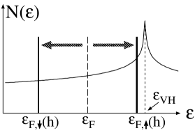
Figure 3: Schematic view of the density of states $N(\epsilon)$ considered in this paper. The density of states has a peak at van Hove energy $\epsilon_{\rm VH}=4(t^{\prime}-t")$, and a spin-dependent Fermi energy $\epsilon_{{\rm F},\uparrow}$ touches $\epsilon_{\rm VH}$ under magnetic fields. In the situation shown here, the up-spin is assigned as the “active” spin component.

As discussed in Ref. Valenzuela, , Eq. (17) contains a phase with $d_{x^{2}-y^{2}}$-wave PI as a mean field solution. This phase appears when the Fermi energy coincides with van Hove energy Halboth $\epsilon_{\rm VH}=4(t^{\prime}-t^{\prime\prime})$. In this paper we consider a situation where the zero-magnetic-field Fermi energy $\epsilon_{\rm F}$ does not satisfies the “van Hove condition” ($\epsilon_{\rm F}\neq\epsilon_{\rm VH}$), but a moderately large external magnetic field $h$ tunes one of the spin-dependent Fermi energies $\epsilon_{{\rm F},\sigma^{*}}(h)$ to a van Hove condition. In this situation, the spin component $\sigma^{*}$ satisfying $\epsilon_{{\rm F},\sigma^{*}}(h)=\epsilon_{\rm VH}$ is relevant to the occurrence of the PI, and we hereafter consider only the “active” spin component $\sigma^{*}$. The antiferromagnetic correlations described by the on-site repulsion $H_{U}$ are suppressed because of the polarization under the strong external magnetic field. Although the ferromagnetic state could compete with the PI, we discuss the case where the PI is stabilized by choosing the parameters $V\approx U/2$.

We first make a mean field decoupling by taking the two contractions,

$$H_{V} = V\sum_{\langle{\bm{r}}_{i},{\bm{r}}_{j}\rangle}\sum_{\sigma,\sigma^{\prime}}\mathchoice{\vbox{\hbox to0.0pt{\kern 0.0pt\kern 2.16377pt\hbox{\vrule width=0.50003pt,height=0.0pt,depth=8.61108pt\vrule width=65.34712pt,height=0.0pt,depth=0.50003pt\vrule width=0.50003pt,height=0.0pt,depth=8.61108pt}\hss}\vskip 2.15277pt\vskip 4.30554pt}}{\vbox{\hbox to0.0pt{\kern 0.0pt\kern 2.16377pt\hbox{\vrule width=0.50003pt,height=0.0pt,depth=8.61108pt\vrule width=65.34712pt,height=0.0pt,depth=0.50003pt\vrule width=0.50003pt,height=0.0pt,depth=8.61108pt}\hss}\vskip 2.15277pt\vskip 4.30554pt}}{\vbox{\hbox to0.0pt{\kern 0.0pt\kern 1.51463pt\hbox{\vrule width=0.50003pt,height=0.0pt,depth=8.61108pt\vrule width=45.95236pt,height=0.0pt,depth=0.50003pt\vrule width=0.50003pt,height=0.0pt,depth=8.61108pt}\hss}\vskip 2.15277pt\vskip 3.01389pt}}{\vbox{\hbox to0.0pt{\kern 0.0pt\kern 1.08188pt\hbox{\vrule width=0.50003pt,height=0.0pt,depth=8.61108pt\vrule width=35.81546pt,height=0.0pt,depth=0.50003pt\vrule width=0.50003pt,height=0.0pt,depth=8.61108pt}\hss}\vskip 2.15277pt\vskip 2.15277pt}}\mathchoice{\vbox{\hbox to0.0pt{\kern 21.3129pt\kern 2.16377pt\hbox{\vrule width=0.50003pt,height=0.0pt,depth=12.91663pt\vrule width=22.02393pt,height=0.0pt,depth=0.50003pt\vrule width=0.50003pt,height=0.0pt,depth=12.91663pt}\hss}\vskip 2.15277pt\vskip 4.30554pt}}{\vbox{\hbox to0.0pt{\kern 21.3129pt\kern 2.16377pt\hbox{\vrule width=0.50003pt,height=0.0pt,depth=12.91663pt\vrule width=22.02393pt,height=0.0pt,depth=0.50003pt\vrule width=0.50003pt,height=0.0pt,depth=12.91663pt}\hss}\vskip 2.15277pt\vskip 4.30554pt}}{\vbox{\hbox to0.0pt{\kern 14.98212pt\kern 1.51463pt\hbox{\vrule width=0.50003pt,height=0.0pt,depth=12.91663pt\vrule width=15.48999pt,height=0.0pt,depth=0.50003pt\vrule width=0.50003pt,height=0.0pt,depth=12.91663pt}\hss}\vskip 2.15277pt\vskip 3.01389pt}}{\vbox{\hbox to0.0pt{\kern 11.60315pt\kern 1.08188pt\hbox{\vrule width=0.50003pt,height=0.0pt,depth=12.91663pt\vrule width=12.11102pt,height=0.0pt,depth=0.50003pt\vrule width=0.50003pt,height=0.0pt,depth=12.91663pt}\hss}\vskip 2.15277pt\vskip 2.15277pt}}c^{{\dagger}}_{\sigma}({\bm{r}}_{i})c_{\sigma}({\bm{r}}_{i})c^{{\dagger}}_{\sigma^{\prime}}({\bm{r}}_{j})c_{\sigma^{\prime}}({\bm{r}}_{j}),$$ (23)

one by one. This yields the following mean field Hamiltonian,

$$H^{\rm MF}_{V} = -\frac{1}{2}\sum_{{\bm{r}}_{i}}\sum_{{\bm{\delta}}=\pm\hat{\bm{x}},\hat{\bm{y}}}\eta_{\delta}({\bm{r}}_{i})c^{{\dagger}}_{\sigma^{*}}({\bm{r}}_{i})c_{\sigma^{*}}({\bm{r}}_{i}+{\bm{\delta}}),$$ (24)

where $\eta_{\delta}({\bm{r}}_{i})=V\langle c^{{\dagger}}_{\sigma^{*}}({\bm{r}}_{i}+{\bm{\delta}})c_{\sigma^{*}}({\bm{r}}_{i})\rangle,$ and we have picked up only the “active” spin component $\sigma^{*}$ satisfying the van Hove condition. We further assume that the parity of $\eta_{\delta}$ with respect to ${\bm{\delta}}$ is even (i.e., $\eta_{\delta}=\eta_{-\delta}$). Then, we have

$$H^{\rm MF}_{V} = -\frac{1}{2}\sum_{{\bm{r}}_{i}}\bigg{[}\Big{(}\eta({\bm{r}}_{i})+\eta^{\prime}({\bm{r}}_{i})\Big{)}c^{{\dagger}}_{\sigma^{*}}({\bm{r}}_{i})c_{\sigma^{*}}({\bm{r}}_{i}+\widehat{\bm{x}})$$ (25)

$$+\Big{(}-\eta({\bm{r}}_{i})+\eta^{\prime}({\bm{r}}_{i})\Big{)}c^{{\dagger}}_{\sigma^{*}}({\bm{r}}_{i})c_{\sigma^{*}}({\bm{r}}_{i}+\widehat{\bm{y}})\bigg{]}$$

$$+H.c.,$$

where $\eta({\bm{r}}_{i})=\frac{1}{2}[\eta_{x}({\bm{r}}_{i})-\eta_{y}({\bm{r}}_{i})]$ and $\eta^{\prime}({\bm{r}}_{i})=\frac{1}{2}[\eta_{x}({\bm{r}}_{i})+\eta_{y}({\bm{r}}_{i})]$. Because $\eta^{\prime}$ possesses the four-fold symmetry of the underlying square lattice and can be regarded as a mass renormalization of the quasiparticles, we hereafter neglect it. On the other hand, a nonzero value of $\eta$ corresponds to the deformation of the Fermi surface which expands along the $p_{x}$ axis and shrinks along $p_{y}$ axis (or vice versa) and Eq.(25) describes a $d_{x^{2}-y^{2}}$-wave PI. Going to the momentum representation, we have

$$H^{\rm MF}_{V} = -\sum_{{\bm{q}},{\bm{p}}}d_{\bm{p}}\eta({\bm{q}})c^{{\dagger}}_{{\bm{p}}+{\bm{q}},\sigma^{*}}c_{{\bm{p}},\sigma^{*}},$$ (26)

where $d_{\bm{p}}=\cos p_{x}-\cos p_{y}$, and $\eta({\bm{r}}_{i})=\sum_{\bm{q}}\eta({\bm{q}})e^{{\rm i}{\bm{q}}{\bm{r}}_{i}}$.

Several comments are in order. In a situation where the PI could be stabilized under the zero magnetic field, it would compete Kee08 with the so-called $d$-density wave state, a state with $\eta({\bm{q}}=\pm(\pi,\pi))$. Under a moderately large magnetic field, however, the $d$-density wave state is not expected to be competitive anymore since this state shows diamagnetic properties Nersesyan1 suggesting that such a state is suppressed under sizable magnetic fields. Solving these problems is beyond our scope because it would require to include Landau diamagnetism such that the resulting analysis becomes considerably more complicated. Therefore in the following we assume that a uniform $\eta({\bm{q}}=0)$ gives the ground state, and the momentum ${\bm{q}}$ appearing in Eq. (26) is small (i.e., ${\bm{q}}\ll 1$).

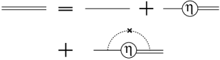
Figure 4: The equation determining the impurity-averaged Green’s function for the “active” spin component $\sigma^{*}$. The single solid line represent the impurity-averaged bare Green’s function [Eq. (22)]. A double solid line, and dotted line with a cross represent the impurity-averaged Green’s function, and impurity scattering, respectively.

The equation determining the impurity-averaged Green’s function for the “active” spin component $\sigma^{*}$ is diagrammatically shown in FIG. 4 where the single solid line represents the impurity-averaged bare Green’s function [Eq. (22)]. Hereafter, we neglect the last diagram in FIG. 4 assuming that the impurity potential is sufficiently weak. Due to the symmetry difference between $\eta$ and the impurity potential, this approximation is exact up to the linear order in $\eta$. Physically this means that the impurity effect on the second order transition line is rigorously treated while the first order transition line may slightly deviate from the exact result. We note here that even with this simplification, the required full numerical calculation is rather involved. With this approximation, the equation for the impurity-averaged Green’s function is solved as

$$G_{\sigma^{*}}({\bm{p}},{\rm i}\varepsilon_{n}) = \frac{1}{[G_{\sigma^{*}}^{(0)}({\bm{p}},{\rm i}\varepsilon_{n})]^{-1}+d_{\bm{p}}\eta},$$ (27)

where the order parameter $\eta$ is determined by the following self-consistent equation

$$\eta = V\int_{{\bm{p}}}d_{\bm{p}}f_{\Gamma}(\xi_{{\bm{p}},\sigma^{*}}-d_{\bm{p}}\eta).$$ (28)

Here we have introduced a shorthand notation $\int_{\bm{p}}=\frac{1}{N}\sum_{\bm{p}}$, and the quantity

$$f_{\Gamma}(\xi_{{\bm{p}},\sigma^{*}}) = T\sum_{\varepsilon_{n}}G^{(0)}_{\sigma^{*}}({\bm{p}},{\rm i}\varepsilon_{n})$$ (29)

may be considered as the impurity-averaged Fermi distribution function. The corresponding mean field free energy is given by

$$\frac{F_{\rm MF}}{N} = \frac{\eta^{2}}{2V}-T\sum_{\varepsilon_{n}}\int_{{\bm{p}}}\ln\frac{|G^{(0)}_{\sigma^{*}}({\bm{p}},{\rm i}\varepsilon_{n})|^{2}}{|G_{\sigma^{*}}({\bm{p}},{\rm i}\varepsilon_{n})|^{2}}.$$ (30)

In the pure limit ($\Gamma\to 0$), the function $f_{\Gamma}$ becomes equal to the Fermi distribution function $f_{0}(x)=(1+e^{(x)/T})^{-1}$ due to the identity $T\sum_{\varepsilon_{n}}G^{(0)}_{\sigma^{*}}({\bm{p}},{\rm i}\varepsilon_{n})=f_{0}(\xi_{{\bm{p}},\sigma^{*}})$. This would simplify the self-consistent equation (28), and the free energy (30) would be reduced to a simpler form $\frac{F_{\rm MF}}{N}=\frac{\eta^{2}}{2V}-T\int_{{\bm{p}}}\ln|(1+e^{-(\xi_{\bm{p}}-d_{\bm{p}}\eta)/T})/({1+e^{-\xi_{\bm{p}}/T}})|$. However because we consider the effect of non-magnetic impurities in this work, we need to use Eqs. (28) and (30).

The mean field phase diagram can be drawn by making a Landau expansion Yamase05 of the free energy (30) as

$$\frac{F_{\rm MF}}{N} \to \frac{F_{\rm GL}}{N}=\left(\frac{a_{\rm GL}}{2}\right)\eta^{2}+\left(\frac{b_{\rm GL}}{4}\right)\eta^{4}\cdots,$$ (31)

where the coefficients $a_{\rm GL}$ and $b_{\rm GL}$ are given by

$$a_{\rm GL} = \frac{1}{V}-\int_{\bm{p}}d^{2}_{\bm{p}}\Big{(}-f^{\prime}_{\Gamma}(\xi_{{\bm{p}},\sigma^{*}})\Big{)},$$ (32)

$$b_{\rm GL} = \frac{1}{3!}\int_{\bm{p}}d^{4}_{\bm{p}}\Big{(}f^{\prime\prime\prime}_{\Gamma}(\xi_{{\bm{p}},\sigma^{*}})\Big{)},$$ (33)

with a convention $f^{\prime}_{\Gamma}(\xi_{{\bm{p}},\sigma})=\frac{\partial}{\partial\xi_{{\bm{p}},\sigma}}f_{\Gamma}(\xi_{{\bm{p}},\sigma})$, etc.

A condition $a_{\rm GL}=0$ defines a second order transition line $T_{c0}(h)$ in the mean field approximation, if the coefficient of the quartic term of the GL free energy ($b_{\rm GL}$) is positive. In case of a negative quartic term the transition becomes of the first order, and the first order transition line $T^{*}_{c}(h)$ is determined by the conditions $F_{\rm MF}(\eta)=0$ and $\partial F_{\rm MF}(\eta)/\partial\eta=0$ for a nonzero $\eta$ where $F_{\rm MF}$ is defined in Eq. (30).

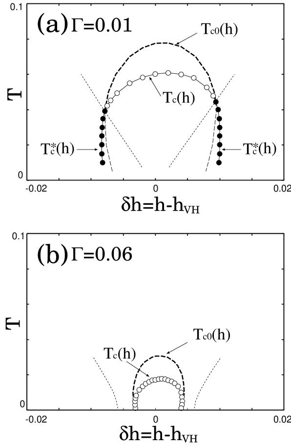
Figure 5: Phase diagrams obtained from Eq. (17) for two different strengths of the impurity scattering, $\Gamma=0.01$ [(a)] and $\Gamma=0.06$ [(b)]. Note that length and energy are measured in unit of the lattice spacing $a$ and the nearest hopping amplitude $t$. We use $U=3.0$ and $V=1.5$ for electron repulsions, and $t^{\prime}=0.4$ and $t^{\prime\prime}=0.2$ for hopping. Two (thick and thin) dashed lines are defined by $a_{\rm GL}=0$ where the thick dashed line represents a mean field second order phase transition line $T_{c0}(h)$ while the thin dashed line is an unphysical one because it is replaced by the following first order transition. A line with full circles show a first order transition line $T^{*}_{c}(h)$ defined by $F_{\rm MF}(\eta)=0$ and $\partial F_{\rm MF}(\eta)/\partial\eta=0$. A line with open circles represents the fluctuation renormalized second order transition line $T_{c}(h)$. A dotted line represents a temperature below which the quartic term $b_{\rm GL}$ [Eq. (33)] of the Ginzburg-Landau free energy becomes negative.

We calculate the mean field phase diagram by using a square mesh of $500\times 500$ in the Brillouin zone. In FIG. 5 (a), we show the calculated mean field phase diagram for a moderately clean sample ($\Gamma=0.01$). Not surprisingly, the phase diagram in this clean case is quite similar to that already obtained in the pure limit ($\Gamma=0$) in the previous work, Yamase07 since as will be discussed below Eq. (37) in the next section, our model is similar to that used in Ref. Yamase07, except for the difference in a spin mixing. The important feature in the phase diagram is that the transition is of second order at higher temperatures while at lower temperatures a first order transition occurs. In the figure, we used a non-zero third-nearest neighbor hopping $t^{\prime\prime}=0.2$. This is because when we use smaller values of $t^{\prime\prime}$, a finite momentum state $\eta({\bm{q}}\neq 0)$ is stabilized due to a nesting condition.

Next let us see how a slight increase in the impurity scattering modifies the mean field phase diagram. Ho08 In FIG. 5 (b), the mean field phase diagram for a dirtier case ($\Gamma=0.06$) is shown. Firstly, we see that the PI is easily suppressed by the increased impurity scattering. This is understandable because the order parameter of the PI and the impurity potential have different symmetry. Hence, the underlying mechanism is analogous to what happens to a disordered $d$-wave superconductor where Anderson’s theorem is violated due to the unconventional nature of the order parameter. Secondly, the first order transition line at low temperatures disappears while the second order transition still survives. These two features concerning impurity effects are important when we discuss the relevance of the PI-scenario to the metamagnetic transition found in Sr₃Ru₂O₇ in Sec. IV.

III.2 Self-consistent Renormalization (SCR) treatment of the Fermi surface fluctuation

In this subsection, we study how the mean field result obtained in the previous subsection is modified by fluctuation effects. Following Refs. Yamase04, and DellAnna06, , we define the (thermal) $d$-wave density correlation function

$$\chi_{d}({\bm{q}},{\rm i}\omega_{m}) = \frac{1}{N}\int_{0}^{1/T}d\tau\;{\rm e}^{{\rm i}\omega_{m}\tau}\langle n_{d}({\bm{q}},\tau)n_{d}(-{\bm{q}},0)\rangle,$$ (34)

where $n_{d}({\bm{q}})=\sum_{{\bm{p}}}d_{{\bm{p}}}c^{\dagger}_{{\bm{p}}+{\bm{q}}/2,\sigma^{*}}c_{{\bm{p}}-{\bm{q}}/2,\sigma^{*}}$ is the $d$-wave density operator in the “active” spin component $\sigma^{*}$. In general, $\chi_{d}$ has the following structure

$$1/\chi_{d} = 1/\chi_{d}^{\rm irr}-V,$$ (35)

where $\chi^{\rm irr}_{d}$ is the irreducible part of $\chi_{d}$. To proceed further to the detailed calculation of $\chi_{d}$, it is convenient to rewrite the interaction Hamiltonian $H_{V}$ in the momentum space,

$$H_{V} = \frac{1}{2N}\sum_{{\bm{p}}_{1},{\bm{p}}_{2},{\bm{p}}_{3}}\sum_{\sigma,\sigma^{\prime}}V_{{\bm{p}}_{1}-{\bm{p}}_{2}}c^{\dagger}_{{\bm{p}}_{1},\sigma}c_{{\bm{p}}_{2},\sigma}$$ (36)

$$\hskip 71.13188pt\times c^{\dagger}_{{\bm{p}}_{3},\sigma^{\prime}}c_{{\bm{p}}_{1}+{\bm{p}}_{3}-{\bm{p}}_{2},\sigma^{\prime}},$$

where $V_{{\bm{p}}}=2V(\cos p_{x}+\cos p_{y})$. Now we decouple $V_{{\bm{p}}_{1}-{\bm{p}}_{2}}$ as $V_{{\bm{p}}_{1}-{\bm{p}}_{2}}=V[d_{{\bm{p}}_{1}}d_{{\bm{p}}_{2}}+s_{{\bm{p}}_{1}}s_{{\bm{p}}_{2}}+p^{(+)}_{{\bm{p}}_{1}}p^{(+)}_{{\bm{p}}_{2}}+p^{(-)}_{{\bm{p}}_{1}}p^{(-)}_{{\bm{p}}_{2}}]$, where $d_{{\bm{p}}}=\cos k_{x}-\cos k_{y}$, $s_{{\bm{p}}}=\cos k_{x}+\cos k_{y}$, and $p^{(\pm)}_{{\bm{p}}}=\sin k_{x}\pm\sin k_{y}$. Because the four van Hove points in the Brillouin zone enhance the interaction with $d_{x^{2}-y^{2}}$ form factor Halboth $d_{{\bm{p}}}$, we hereafter consider only this channel. After changing the ordering of fermion operators and setting ${\bm{p}}_{1}={\bm{p}}+{\bm{q}}/2,{\bm{p}}_{2}={\bm{p}}^{\prime}+{\bm{q}}/2,{\bm{p}}_{3}={\bm{p}}^{\prime}-{\bm{q}}/2$, we have

$$H_{V} \to H^{\prime}_{V}=-\frac{V}{2N}\sum_{{\bm{q}}}n_{d}({\bm{q}})n_{d}(-{\bm{q}}).$$ (37)

This is essentially the same model as used in Refs.Metzner03, and Yamase07, except for the fact that the interaction $H^{\prime}_{V}$ acts only among the active spin component $\sigma^{*}$.

The so-called random phase approximation (RPA) for $\chi_{d}$ is obtained when we adopt the simplest building block

$$\chi^{{\rm irr}}_{d,0}({\bm{q}},{\rm i}\omega_{m}) = -T\sum_{\omega_{m}}\int_{{\bm{p}}}d_{{\bm{p}}}^{2}G_{\sigma^{*}}^{(0)}({\bm{p}},{\rm i}\varepsilon_{n})$$ (38)

$$\hskip 2.84544pt\times G_{\sigma^{*}}^{(0)}({\bm{p}}+{\bm{q}},{\rm i}\varepsilon_{n}+{\rm i}\omega_{m})$$

as the irreducible $\chi^{\rm irr}_{d}$. Hereafter, we write the $d$-wave density correlation function in a dimensionless form by introducing $\widetilde{\chi}_{d}=\chi_{d}/\chi^{\rm irr}_{d,0}$. Then, the RPA $d$-wave density correlation function is given by

$$1/\widetilde{\chi}_{d,{\rm RPA}}({\bm{q}},{\rm i}\omega_{m}) = 1-V\chi^{\rm irr}_{d,0}({\bm{q}},{\rm i}\omega_{m}).$$ (39)

Near the second order PI, the retarded function $\widetilde{\chi}^{R}_{d,{\rm RPA}}({\bm{q}},\omega)=\widetilde{\chi}_{d,{\rm RPA}}({\bm{q}},{\rm i}\omega_{m}\to\omega+{\rm i}0_{+})$ takes the same form as Eq. (8),

$$[\widetilde{\chi}^{R}_{d,{\rm RPA}}({\bm{q}},\omega)]^{-1} = \mu_{0}+\xi_{0}^{2}q^{2}-{\rm i}\frac{\omega}{w_{0}(\widehat{{\bm{q}}})|q|}.$$ (40)

where $\mu_{0}=Va_{\rm GL}\propto T-T_{c0}$ with $a_{\rm GL}$ and $T_{c0}$ being the quadratic coefficient in Eq. (32) and the mean field transition temperature. Also, $\xi_{0}^{2}$ and $w_{0}$ are given by (see Appendix A)

$$\xi_{0}^{2} = V\int_{\bm{p}}d^{2}_{\bm{p}}\Big{[}\frac{f{{}^{\prime\prime\prime}}_{\Gamma}(\xi_{{\bm{p}},\sigma^{*}})}{12}(v_{x}^{2}+v_{y}^{2})$$ (41)

$$\hskip 28.45274pt+\frac{f{{}^{\prime\prime}}_{\Gamma}(\xi_{{\bm{p}},\sigma^{*}})}{4}(M_{x}+M_{y})\Big{]},$$

$$\frac{1}{w_{0}(\widehat{{\bm{q}}})} = V\int_{{\bm{p}}}d^{2}_{{\bm{p}}}\left(\frac{-f^{\prime}_{\Gamma}(\xi_{{\bm{p}},\sigma^{*}})}{2\Gamma/q_{{\rm c}}+{\rm i}{\bm{v}}_{{\bm{p}},\sigma^{*}}\cdot\widehat{{\bm{q}}}}\right),$$ (42)

where $M_{j}=(1/2)\partial^{2}\xi_{\bm{p}}/\partial k_{j}^{2}$ for $j=x,y$ and $q_{{\rm c}}$ is the wavevector cutoff. We note that, as was already mentioned above Eq. (27), neglecting the impurity vertex corrections, Fulde68 which would otherwise transform the dynamical behavior into a diffusive one, remains exact in the calculation of these quantities.

Figure 6: Diagrams for the fluctuation propagator of $d_{x^{2}-y^{2}}$-wave PI [(a) and (b)] and the irreducible $d_{x^{2}-y^{2}}$-wave correlation function giving the mode coupling between fluctuations [(c)]. The solid line represents the impurity-averaged bare Green’s function of quasiparticles, the dashed line the next nearest neighbor repulsion [Eq. (36)].

In the presence of interlayer coupling, the critical behavior is expected to be governed by three-dimensional fluctuations, Hikami80 and we assume in this work an anisotropic three-dimensional (3D) behavior of the fluctuations. Microscopically, the three dimensionality is introduced by adding a $z$-axis dispersion $\delta\epsilon_{P_{z}}=-\delta t\cos(P_{z})$ into Eq. (20). Instead of doing so, however, we here introduce the three dimensionality in a more phenomenological way, by replacing the two-dimensional wavevector ${\bm{q}}$ appearing in $\widetilde{\chi}_{d}({\bm{q}},{\rm i}\omega_{m})$ with a three-dimensional wavevector ${\bm{Q}}^{\prime}=({\bm{q}},Q_{z}/\gamma)$, namely,

$$\widetilde{\chi}_{d}({\bm{q}},{\rm i}\omega_{m}) \to \widetilde{\chi}_{d}({\bm{Q}}^{\prime},{\rm i}\omega_{m}),$$ (43)

where $\gamma=\xi_{0}/\xi_{c0}$ is the anisotropy parameter given by the ratio of the in-plane correlation length to the out-of-plane correlation length. The above procedure is justified at least for a system with anisotropic ellipsoidal 3D Fermi surface. Here we would like to mention the recent proposal in the context of high-$T_{c}$ cuprates Yamase09 that the interlayer-configuration of the nematic order becomes alternate pattern of $\eta>0$ [FIG. 1 (b)] and $\eta<0$ [FIG. 1 (c)]. We do not take into account such a possibility here, since this configuration costs the elastic energy of the crystal lattice. We would like to point out that, while a minor change in the form of the propagator in Eq. (40) is needed if the $d_{x^{2}-y^{2}}$-wave PI has such a configuration, the main result of this paper is not changed, at least qualitatively.

Now we consider the effect of mode coupling between the fluctuations. In the bosonic languages, Hertz76 ; Millis93 this is given by the self-energy renormalization for the fluctuation propagator coming from the quartic term of the action. In the fermionic languages which we adopt in this work, the corresponding mode coupling is given by the three diagrams Kawabata shown in Fig. 6, which give

$$\widetilde{\chi}^{\rm irr}_{d} = \widetilde{\chi}^{\rm irr}_{d,0}+\delta\widetilde{\chi}^{\rm irr}_{d},$$ (44)

$$\delta\widetilde{\chi}^{\rm irr}_{d} = -3b_{\rm GL}\;V^{2}\;T\sum_{\omega_{m}}\int\frac{\gamma d^{3}Q^{\prime}}{(2\pi)^{3}}\;\widetilde{\chi}_{d}({\bm{Q}}^{\prime},{\rm i}\omega_{m}),$$ (45)

where $b_{\rm GL}$ is the coefficient of the quartic term in the Ginzburg-Landau free energy given by Eq. (31). Substituting Eq. (44) into Eq. (35) and expanding it in terms of $\delta\chi^{\rm irr}_{d}$, we obtain

$$1/\widetilde{\chi}_{d} = 1/\widetilde{\chi}_{d,{\rm RPA}}-\delta\widetilde{\chi}^{\rm irr}_{d},$$ (46)

where $\delta\widetilde{\chi}^{\rm irr}_{d}$ also depends on $\widetilde{\chi}_{d}$ through Eq. (45).

As discussed in Ref. Millis93, , the SCR formalism is a self-consistent one-loop approximation for the mass renormalization

$$\mu = 1/\widetilde{\chi}_{d}({\bm{Q}}^{\prime}={\bm{0}},{\rm i}\omega_{m}=0).$$ (47)

Substituting Eq. (47) into Eq. (46) and making the contour deformation for the Matsubara summation, we obtain the following SCR equation to determine $\mu$,

$$\mu = \mu_{0}+\delta\mu,$$ (48)

$$\delta\mu = 3b_{\rm GL}V^{2}\int_{-\infty}^{\infty}\frac{d\omega}{2\pi}\int_{0}^{Q^{\prime}_{\rm c}}\frac{\gamma d^{3}Q^{\prime}}{(2\pi)^{3}}\coth\left(\frac{\omega}{2T}\right)$$ (49)

$$\hskip 56.9055pt\times{\rm Im}\widetilde{\chi}^{R}_{d}({\bm{Q}}^{\prime},\omega),$$

where ${Q}^{\prime}_{\rm c}$ is the wavevector cutoff. The frequency integral in Eq. (49) can be performed using the relation $\coth(x/2)=1+2/({\rm e}^{z}-1)$ and $\int_{0}^{\infty}dx({\rm e}^{x}-1)^{-1}[x/(x^{2}+c^{2})]=(1/2)[\ln(c/2\pi)-\pi/c-\Psi(c/2\pi)]$. Then, introducing the normalized wavevector $\widetilde{{\bm{Q}}}^{\prime}=\xi_{0}{\bm{Q}}^{\prime}$, the final result can be written as

$$\delta\mu = \frac{3b_{\rm GL}V^{2}\gamma}{2\pi^{2}\xi_{0}^{3}}\int_{0}^{\widetilde{Q}^{\prime}_{\rm c}}(\widetilde{Q}^{\prime 2}d\widetilde{Q}^{\prime})\left(\frac{T}{\mu_{\widetilde{Q}^{\prime}}}\right)$$ (50)

$$\hskip 28.45274pt\times 2Z_{\widetilde{Q}^{\prime}}\Big{(}\ln Z_{\widetilde{Q}^{\prime}}-\frac{1}{2Z_{\widetilde{Q}^{\prime}}}-\Psi(Z_{\widetilde{Q}^{\prime}})\Big{)},$$

where $\Psi(Z)$ is the digamma function, $\mu_{\widetilde{Q}^{\prime}}=\mu+\widetilde{Q}^{\prime 2}$, $Z_{\widetilde{Q}^{\prime}}=\mu_{\widetilde{Q}^{\prime}}w_{0}|\widetilde{Q}^{\prime}|/(2\pi T\xi_{0})$. When the condition $Z_{\widetilde{Q}^{\prime}}\ll 1$ is satisfied, we can set $2Z_{\widetilde{Q}^{\prime}}[\ln Z_{\widetilde{Q}^{\prime}}-(1/2)Z_{\widetilde{Q}^{\prime}}-\Psi(Z_{\widetilde{Q}^{\prime}})]\to 1$ and the above expression reproduces the result of the Hartree approximation for the mass renormalization due to classical fluctuations, Chaikin which means that Eq. (50) can describe both quantum and classical fluctuation regions.

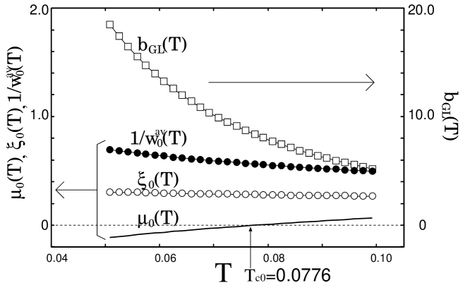
Figure 7: Temperature dependences of parameters characterizing the bare $d$-wave density correlation function; the mass term $\mu_{0}$, correlation length $\xi_{0}$, and damping coefficient $w_{0}$. The mode-coupling parameter $b_{\rm GL}$ is also plotted. The parameters used in this figure are the same as in FIG. 5 (a).

In FIG. 7, we plot the temperature dependences of several parameters characterizing the bare $d$-wave density correlation function, the mass term $\mu_{0}$, correlation length $\xi_{0}$, and damping coefficient $w_{0}$, as well as the mode-coupling parameter $b_{\rm GL}$. Strictly speaking, $w_{0}(\widehat{{\bm{q}}})$ in Eq. (42) depends on $\widehat{{\bm{q}}}$ but we average them using two values at ${\bm{q}}=\widehat{\bm{x}}$ and ${\bm{q}}=(\widehat{\bm{x}}+\widehat{\bm{y}})/2$, i.e., $w_{0}({\bm{q}})\to w_{0}^{\rm av}=(1/2)\{w_{0}(\widehat{\bm{x}})+w_{0}[(\widehat{\bm{x}}+\widehat{\bm{y}})/2]\}$. From the figure, we can see the following three points. First, as was already discussed in the pure limit Yamase07 ($\Gamma=0$), the bare mass term $\mu_{0}$ is as small as $\sim 0.1$ in a wide temperature region above the mean field transition temperature $T_{c0}$. Second, the correlation length is shorter than the lattice spacing $a=1$, which can be understood from Eqs. (41) because the quasiparticle velocity $|{\bm{v}}_{\bm{p}}|$ is quite small near van Hove filling. Third, the mode coupling parameter $b_{\rm GL}$ is one order of magnitude larger than other parameters ($\mu_{0},\xi_{0},1/w_{0}$) characterizing Gaussian fluctuations. All these features result in strong fluctuations near the $d_{x^{2}-y^{2}}$ PI.

In FIG. 8, we plot the temperature dependence of the renormalized mass $\mu=1/\widetilde{\chi}_{d}({\bm{Q}}^{\prime}={\bm{0}},{\rm i}\omega_{m}=0)$ as well as the bare mass $\mu_{0}=1/\widetilde{\chi}_{d,{\rm RPA}}({\bm{Q}}^{\prime}={\bm{0}},{\rm i}\omega_{m}=0)$. As expected, $\mu(T)$ coincides with $\mu_{0}(T)$ well above the mean field transition temperature $T_{c0}$ but it deviates from the mean field result near and below $T_{c0}$. From the figure we determine the fluctuation-renormalized transition temperature $T_{c}$ by a condition $\mu(T_{c})<10^{-3}$. In FIG. 5 we have also plotted $T_{c}(h)$ thus determined. We can see that the fluctuation region becomes smaller on approaching the first order transition line.

Figure 8: Temperature dependence of the renormalized mass $\mu=1/\widetilde{\chi}_{d}({\bm{Q}}^{\prime}={\bm{0}},{\rm i}\omega_{m}=0)$ (open circles) and the bare mass $\mu_{0}=1/\widetilde{\chi}_{d,{\rm RPA}}({\bm{Q}}^{\prime}={\bm{0}},{\rm i}\omega_{m}=0)$ (dashed line) for $\Gamma=0.01$ [(a)] and $\Gamma=0.06$ [(b)]. We use the wavevector cutoff ${Q}^{\prime}_{\rm c}=0.0555$ and anisotropy parameter $\gamma=5$, and other parameters are the same as in FIG. 5. Two curves are calculated along a fixed magnetic field $h=h_{\rm VH}$ where the mean field transition is always of second order. The fluctuation-renormalized transition temperature $T_{c}$ is determined by a condition $\mu(T_{c})<10^{-3}$.

III.3 Fluctuation sound attenuation

We consider the electron-phonon interaction following the argument given by Walker, Smith and Samokhin, Walker01 and begin with the tight-binding Hamiltonian

$$H_{\rm el-ph} = \sum_{\bm{\delta}}{\bm{g}}({\bm{\delta}})\sum_{{\bm{r}}_{i},\sigma}\Big{(}{\bm{u}}({\bm{r}}_{i})-{\bm{u}}({\bm{r}}_{i}+{\bm{\delta}})\Big{)}$$ (51)

$$\times \Big{(}c^{{\dagger}}_{\sigma}({\bm{r}}_{i})c_{\sigma}({\bm{r}}_{i}+{\bm{\delta}})+c^{{\dagger}}_{\sigma}({\bm{r}}_{i}+{\bm{\delta}})c_{\sigma}({\bm{r}}_{i})\Big{)},$$

where ${\bm{u}}({\bm{r}}_{i})$ is the displacement of the ion at ${\bm{r}}_{i}$, ${\bm{\delta}}$ is the lattice vector, ${\bm{g}}({\bm{\delta}})={\bf\nabla}t({\bm{\delta}})$ with the hopping amplitude $t({\bm{\delta}})$ between site ${\bm{r}}_{i}$ and ${\bm{r}}_{i}+{\bm{\delta}}$. Following the procedure in Ref. Walker01, and neglecting umklapp processes, the interaction between electrons and a sound wave with wavevector ${\bm{K}}$ and polarization $\nu$ is given by

$$H_{\rm el-ph} = \frac{1}{\sqrt{N}}\sum_{{\bm{P}},{\bm{K}},\sigma}F_{\{\widehat{{\bm{K}}},\nu\}}({\bm{P}})$$ (52)

$$\hskip 28.45274pt\times\sqrt{\frac{\omega^{(0)}_{{\bm{K}},\nu}}{2}}B_{{\bm{K}},\nu}c^{\dagger}_{{\bm{P}}+{\bm{K}},\sigma}c_{{\bm{P}},\sigma},$$

where $B_{{\bm{K}},\nu}=b_{{\bm{K}},\nu}-b^{\dagger}_{-{\bm{K}},\nu}$ with the phonon annihilation operator $b_{{\bm{K}},\nu}$, $\widehat{\bm{e}}_{\nu}$ is the polarization vector, and the electron-phonon vertex function $F_{\{\widehat{{\bm{K}}},\nu\}}({\bm{P}})$ is given by

$$F_{\{\widehat{{\bm{K}}},\nu\}}({\bm{P}}) = \frac{-2}{\sqrt{\rho_{\rm ion}s_{\nu}^{2}}}\sum_{\bm{\delta}}(\widehat{{\bm{K}}}\cdot\widehat{\bm{\delta}})(\widehat{\bm{e}}_{\nu}\cdot{\bm{g}}({\bm{\delta}}))$$ (53)

$$\hskip 56.9055pt\times\cos({\bm{P}}\cdot{\bm{\delta}}).$$

Here, all momenta denoted by capital letters are 3D vectors. However, we consider below the case where the wavevector and the polarization vector of a sound wave lie within a conducting layer because interesting results come out in this case, and we set in the following ${\bm{P}}=({\bm{p}},0)$, ${\bm{K}}=({\bm{k}},0)$, etc. In this work we consider the electron-phonon coupling through at most the next nearest neighbor interactions. Assuming that ${\bm{g}}({\bm{\delta}})$ is proportional to $\widehat{\bm{\delta}}$, we make an expansion ${\bm{g}}({\bm{\delta}})=g_{\rm n.n.}\widehat{\bm{\delta}}_{\rm n.n.}+g_{\rm n.n.n.}\widehat{\bm{\delta}}_{\rm n.n.n.}$ where $g_{\rm n.n.}(g_{\rm n.n.n.})$ is the coupling constant through the nearest (next nearest) neighbor interactions.

Then, for transverse phonons propagating along the $[100]$ direction, because the coupling via the nearest neighbor interaction disappears in this case, the dominant coupling is given by the next nearest neighbor interactions as

$$F_{T100}({\bm{p}}) = \Upsilon_{T100}(2\sin p_{x}\sin p_{y}),$$ (54)

while for transverse phonons propagating along the $[110]$ direction,

$$F_{T110}({\bm{p}}) = \Upsilon_{T110}(\cos p_{x}-\cos p_{y}),$$ (55)

where $\Upsilon_{T100}=-g_{\rm n.n.n.}\sqrt{L_{z}/\rho_{\rm ion}(s_{T100})^{2}}$ [$\Upsilon_{T110}=-g_{\rm n.n}\sqrt{L_{z}/\rho_{\rm ion}(s_{T110})^{2}}$] with system’s $c$-axis dimension $L_{z}$. The electron-phonon vertex function for the longitudinal phonons is given by

$$F_{L}({\bm{p}}) = \Upsilon_{L}(\widehat{q}_{x}^{2}\cos p_{x}+\widehat{q}_{y}^{2}\cos p_{y})$$ (56)

with $\Upsilon_{L}=-g_{\rm n.n.}\sqrt{L_{z}/\rho_{\rm ion}(s_{L})^{2}}$. The important point here is that in each case $F_{\{\widehat{{\bm{K}}},\nu\}}({\bm{p}})$ can be expressed as $F_{\{\widehat{{\bm{K}}},\nu\}}({\bm{p}})=\Upsilon\,W_{\bm{p}}$ with a form factor $W_{\bm{p}}$ and the corresponding electron-phonon coupling constants $\Upsilon$. For $T100$ phonons, $W_{\bm{p}}$ is equal to the $d_{xy}$-symmetry form factor $d^{\prime}_{\bm{p}}=2\sin p_{x}\sin p_{y}$, while it is equal to the $d_{x^{2}-y^{2}}$-wave form factor $d_{\bm{p}}$ for $T110$ phonons. In case of longitudinal sounds, $W_{\bm{p}}=s_{\bm{p}}+d_{\bm{p}}$ for $L100$ phonons while $W_{\bm{p}}=s_{\bm{p}}$ for $L110$ phonons where $s_{\bm{p}}$ is defined below Eq. (36). We note that the inclusion of an isotropic vertex function into Eq. (56), which ensures the charge neutral condition Walker01 for longitudinal phonons, does not change the main result discussed below.

Using the electron-phonon interaction (52), the sound attenuation is calculated from the phonon Green’s function

$$[D_{\nu}({\bm{k}},{\rm i}\Omega_{m})]^{-1} = [D_{\nu}^{(0)}({\bm{k}},{\rm i}\Omega_{m})]^{-1}-\Pi_{\nu}({\bm{k}},{\rm i}\Omega_{m}),$$ (57)

where $D_{\nu}^{(0)}({\bm{k}},{\rm i}\Omega_{m})=-(\omega^{(0)}_{{\bm{k}},\nu})^{2}/[{\Omega_{m}^{2}+(\omega^{(0)}_{{\bm{k}},\nu})^{2}}]$ is the bare phonon Green’s function, and $\Pi_{\nu}({\bm{k}},{\rm i}\Omega_{m})$ is the phonon self-energy. The retarded phonon self-energy, $\Pi_{\nu}^{R}({\bm{k}},{\rm i}\Omega_{m})=\Pi_{\nu}({\bm{k}},{\rm i}\Omega_{m}\to\Omega+{\rm i}0_{+})$, determines the phonon lifetime as $1/\tau_{{\rm ph},\nu}=-(\omega^{(0)}_{{\bm{k}},\nu})^{2}\frac{1}{\Omega}{\rm Im}\Pi_{\nu}^{R}({\bm{k}},\Omega)$, and the sound attenuation $\alpha_{\nu}({\bm{k}})$ for the phonon with wave vector ${\bm{k}}$ and polarization $\nu$ is given by

$$\alpha_{\nu}({\bm{k}}) = -\left(\frac{(\omega^{(0)}_{{\bm{k}},\nu})^{2}}{s^{(0)}_{\nu}}\right)\frac{1}{\Omega}{\rm Im}\Pi^{R}_{\nu}({{\bm{k}}},\Omega).$$ (58)

Strictly speaking, the sound velocity in Eq. (58) should be understood as a renormalized one,

$$s_{\nu} = s^{(0)}_{\nu}\sqrt{1-{\rm Re}\Pi^{R}_{\nu}({{\bm{k}}},\Omega\to 0)},$$ (59)

with the bare velocity $s^{(0)}_{\nu}$. However, because the renormalization of the sound velocity due to the collective fluctuation is usually quite small in the experimental resolution Luethi70 [$(s_{\nu}-s^{(0)}_{\nu})/s^{(0)}_{\nu}\approx 10^{-3}-10^{-4}$], we use the bare sound velocity in Eq. (58). Note however that the unrenormalized sound velocity should be used only in Eq. (58). As mentioned at the end of Sec. II, the measurement of the softening of the sound velocity is also a key experiment to detect the $d_{x^{2}-y^{2}}$-wave PI.

Consider first the sound attenuation caused by itinerant electrons in the absence of the $d_{x^{2}-y^{2}}$-wave PI. In this case the irreducible phonon self-energy is given by AGD [FIG. 9(a)]

$$\Pi^{(0)}_{\nu}({\bm{k}},{\rm i}\Omega_{m}) = \Upsilon^{2}\;T\sum_{\varepsilon_{n}}\int_{{\bm{p}}}W_{\bm{p}}^{2}\;G_{\sigma^{*}}^{(0)}({\bm{p}},{\rm i}\varepsilon_{n})$$ (60)

$$\hskip 28.45274pt\times G_{\sigma^{*}}^{(0)}({\bm{p}}+{\bm{k}},{\rm i}\varepsilon_{n}+{\rm i}\Omega_{m}).$$

This gives the sound attenuation without the Fermi surface fluctuations, $\alpha^{\rm MF}_{\nu}({\bm{k}})=-[(\omega^{(0)}_{{\bm{k}},\nu})^{2}/s_{\nu}]\frac{1}{\Omega}{\rm Im}\Pi^{(0)R}_{\nu}({{\bm{k}}},\Omega)$.

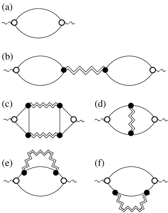
Figure 9: Diagrams for the phonon self-energy $\Pi_{\nu}({\bm{k}},{\rm i}\Omega_{m})$. An open circle represents the electron-phonon vertex in Eq. (53), a full circle the $d_{x^{2}-y^{2}}$-wave vertex $d_{\bm{p}}$, a wavy line the phonon Green’s function, and a double zigzag line the fluctuation propagator defined in FIG. 6.

Now we consider the effect of the $d_{x^{2}-y^{2}}$-wave PI. The relevant diagrams are shown in FIG. 9(b)-(f) where we have neglected impurity vertex corrections due to the reason mentioned above Eq. (27). The simplest diagram is given by FIG. 9(b) which corresponds to the sound attenuation derived from the mode-coupling term (2). Diagram (b) gives the sound attenuation derived from the mode-coupling term (14), and is analogous to the Aslamazov-Larkin diagram Aslamazov for the fluctuation conductivity in a superconductor. Here we have neglected the vertex corrections due to mode-coupling [e.g., FIG. 1(c) in Ref. Ramazashvili, ]. Diagrams (d)-(f) give the contributions which are not described by the phenomenological (bosonic) argument in Sec. II, and analogous to the Maki-Thompson diagram Maki68 ; Thompson70 [diagram (d)] and density of states diagrams Abrahams70 [diagram (e) and (f)]. Note however that the analytical expression of each diagram is different from that of a superconducting fluctuation contribution because the PI is a kind of diagonal long range order while the superconductivity is an off-diagonal long range order.

For the moment, we focus on the transverse sound attenuation because it is this case where the fluctuation sound attenuation is propagation-direction selective. We first consider diagram (b). For the transverse sound along $[100]$ direction, because the electron-phonon vertex function $F_{T100}({\bm{p}})$ [Eq. (54)] has the $d_{xy}$-symmetry, the phonon self-energy does not couple to the collective fluctuation of the $d_{x^{2}-y^{2}}$-wave PI. Hence the phonon self-energy has no divergent contribution, and is given by

$$\Pi_{T100}({\bm{k}},{\rm i}\Omega_{m}) = \Pi^{(0)}_{T100}({\bm{k}},{\rm i}\Omega_{m}),$$ (61)

where $\Pi^{(0)}_{T100}$ is defined in Eq. (60) with $W_{\bm{p}}=d^{\prime}_{\bm{p}}$. On the other hand, the transverse sound along $[110]$ direction does couple to the $d_{x^{2}-y^{2}}$-wave Fermi surface fluctuation because the electron-phonon vertex function $F_{T110}({\bm{p}})$ is proportional to the $d_{x^{2}-y^{2}}$-wave form factor. This gives the divergent phonon self-energy

$$\Pi_{T110}({\bm{k}},{\rm i}\Omega_{m}) = -(\Upsilon_{T110})^{2}\chi_{d}({\bm{k}},{\rm i}\Omega_{m}),$$ (62)

where $\chi_{d}({\bm{k}},{\rm i}\Omega_{m})$ behaves as Eq. (8) near the second order transition.

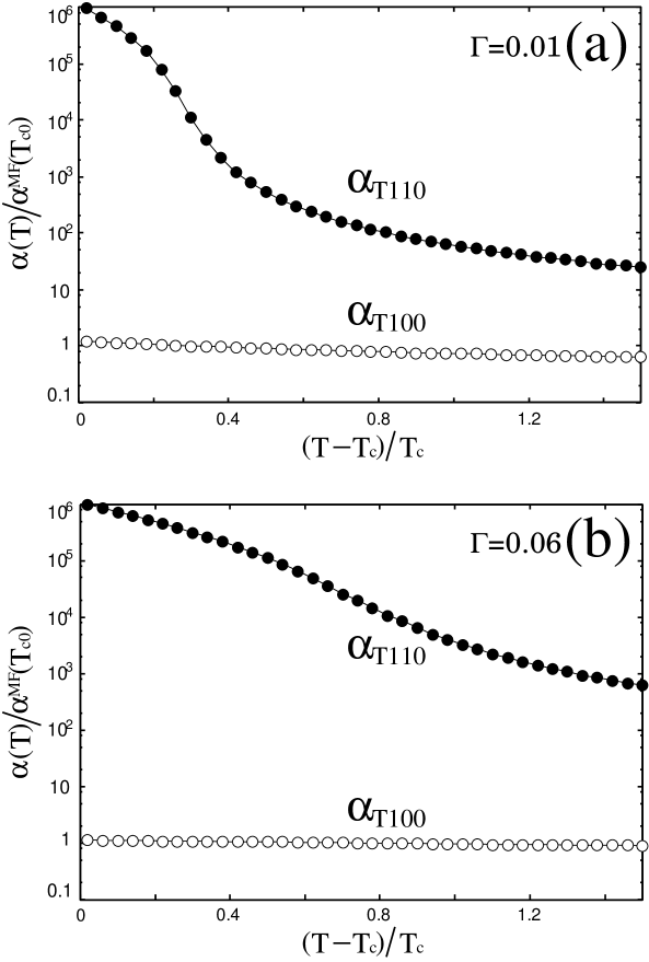
Figure 10: Calculated ultrasound attenuation for $T100$ phonons (open circles) and $T110$ phonons (full circles) for $\Gamma=0.01$ [(a)] and $\Gamma=0.06$ [(b)] at constant field $h=h_{\rm VH}$. The parameters used in this figure are the same as in FIG. 5 and FIG. 8. The data are normalized by $\alpha^{\rm MF}$ at the mean field transition temperature $T_{c0}$ where $\alpha^{\rm MF}$ is defined below Eq. (60).

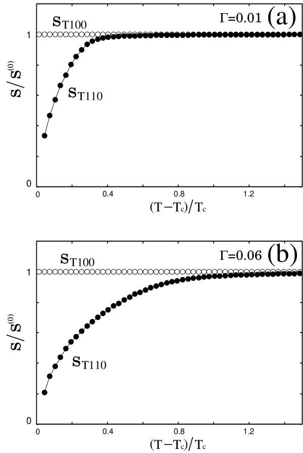
Figure 11: Calculated ultrasound velocity for $T100$ phonons (open circles) and $T110$ phonons (full circles) for $\Gamma=0.01$ [(a)] and $\Gamma=0.06$ [(b)] at constant field $h=h_{\rm VH}$. The parameters used in this figure are the same as in FIG. 5 and FIG. 8. The data are normalized by the bare sound velocity $s^{(0)}$. Here, we have used a moderately large electron-phonon coupling constant $\Upsilon^{2}=0.001$ to enlarge the signal, whereas the actual softening would be much smaller. Luethi70

Next we consider diagram (c). In this case, it is easy to show that the triangle blocks in this diagram vanish for both $T100$ and $T110$ phonons, hence there is no contribution from this diagram. This is consistent with the argument in Sec.II that Eq. (14) couples only to the longitudinal sound, because diagram (b) gives the sound attenuation derived from this mode-coupling term (14).

We then consider diagrams (d)-(f) which were not taken into account in the phenomenological argument in Sec. II. Note that if we pick up only the contribution just at the Fermi surface assuming a constant density of states, then we can show that diagram (d) and diagrams (e) and (f) cancel. However, once we include the energy dependence of the density of states, there is a nonzero contribution from these diagrams as in the case of the quartic term of the GL functional. By power counting, we can show that these diagrams give a logarithmically divergent sound attenuation $\alpha_{T}\sim\ln\mu$ where $\mu$ is the renormalized mass term (47). We think that in the actual experiment this logarithmic divergence is negligible compared with the stronger divergence caused by Eq. (62).

Now we come to the case with longitudinal sound modes. Concerning the fluctuation contribution to the longitudinal sound attenuation, it is sufficient to consider diagram (c) in FIG. 9 irrespective of the propagation direction because as you can see in the following this diagram always gives the divergent behavior with the same exponent. After analytical continuation, diagram (c) gives

$$\Pi_{L}^{R}({\bm{k}},\Omega) \sim -{\rm i}\Omega{\cal B}^{2}\int\frac{d\omega}{\sinh^{2}(\frac{\omega}{2T})}\int d^{3}Q^{\prime}\Big{[}{\rm Im}\chi_{d}^{R}({\bm{Q}}^{\prime},\omega)\Big{]}^{2},$$ (63)

where ${\cal B}=\Upsilon_{L}\sum_{\varepsilon_{n}}\int_{\bm{p}}W_{\bm{p}}d_{\bm{p}}^{2}[G^{(0)}({\bm{p}},{\rm i}\varepsilon_{n})]^{3}=\frac{\Upsilon_{L}}{2}\int_{\bm{p}}W_{\bm{p}}d_{\bm{p}}^{2}f^{\prime\prime}_{\Gamma}(\xi_{{\bm{p}},\sigma^{*}})$ comes from the triangle block in the diagram and ${\bm{Q}}^{\prime}=({\bm{q}},Q_{z}/\gamma)$ is the rescaled three-dimensional wavevector introduced in Eq. (43). Roughly speaking, ${\cal B}$ is proportional to the degree of particle-hole asymmetry, and in case of a perfect particle-hole symmetry this contribution vanishes. By power counting, we can show that this gives a divergent sound attenuation $\alpha_{L}\sim\mu^{-2}$ where $\mu$ is the renormalized mass term (47). Therefore, as was already discussed in Sec. II, the longitudinal sound attenuation always show a divergent behavior on approaching a second order PI.

To summarize, a microscopic calculation of the fluctuation sound attenuation in this subsection gives the same result as obtained by a phenomenological argument in Sec. II. Results of this subsection coincide with the main results in Sec. II, i.e., Eqs. (11), (13) and (15), if we replace the bare mass $\mu_{0}$ with the renormalized mass $\mu$.

In FIG.10 we plot the transverse sound attenuation along $[100]$ and $[110]$ directions as functions of temperature. We also plot in FIG.11 the transverse sound velocities along $[100]$ and $[110]$ directions as functions of temperature. As was already discussed in Sec. II, there is a fluctuation contribution to $[110]$ phonons while there is no contribution to $[110]$ phonons. Comparing data for a cleaner system [FIG.10(a)] to that for a dirtier system [FIG.10(b)], we see that the dirtier system shows broader fluctuation behavior in the reduced temperature $(T-T_{c})/T_{c}$.

IV Discussion and Conclusion

We have studied the effect on sound properties of the Fermi surface fluctuations near a $d_{x^{2}-y^{2}}$-wave PI, and discussed that there is a propagation-direction-dependent selection rule in the fluctuation transverse sound attenuation and sound velocity softening. As is shown in FIG. 2, FIG. 10, and FIG. 11, the transverse sound attenuation and sound velocity softening along $[110]$ direction are enhanced by the Fermi surface fluctuations while those along $[100]$ direction are not affected. Also it was argued that there are always fluctuation contributions to the longitudinal sound attenuation and sound velocity softening. We note that a qualitatively similar conclusion can be reached for a second order structural transition which breaks the lattice symmetry in the same way, but is not caused by a Fermi surface instability. Such a transition would not be identified as a genuine Pomeranchuk instability.

As was already mentioned in Sec. I, the possibility of the $d_{x^{2}-y^{2}}$-wave PI discussed in this paper has been debated Grigera04 ; Kee05 ; Honerkamp05 ; Borzi07 ; Yamase07 ; Doh07 ; Puetter07 as a possible explanation for the anomalous phase found in Sr₃Ru₂O₇ under strong magnetic fields, and it provides us with a good opportunity to apply our results. In earlier experiments for this material, a metamagnetic transition was found Perry01 ; Grigera01 at a magnetic field $B_{m}$ where the magnetization shows a steep jump. Since several non-Fermi-liquid properties are observed around $B_{m}$, this system was originally discussed in terms of the metamagnetic quantum critical point, Millis02 and the importance of van Hove singularity for the metamagnetic transition was discussed. Binz04 However, the subsequent experiments using an ultra-pure sample found at least two transitions, Ohmichi03 ; Perry04 and later on it was revealed Grigera04 that the two transitions reflect the boundary of a new ordered phase which is accompanied by metamagnetic transitions. Based on a consideration on resistivity data, it was proposed Grigera04 and demonstrated Kee05 that the observed new phase can be an ordered state with $d_{x^{2}-y^{2}}$-wave PI.

On this background, it is tempting to compare our results with the experiments for bilayer ruthenate Sr₃Ru₂O₇. Firstly, as was already discussed in Ref. Yamase07, , the calculated phase diagram [FIG. 5 (a)] looks quite similar to what was observed in experiments (Fig. 3 in Ref. Grigera04, ). Secondly, the earlier experiments can be interpreted as a result of the impurity effects which narrow the area of the ordered phase [FIG. 5 (b)], because two closely located transition lines (beyond the experimental resolution) would look like a single transition line in experiments. Thirdly, the non-Fermi-liquid behaviors observed in resistivity, Grigera01 ; Perry01 ; Zhou04 specific heat, Grigera01 ; Zhou04 ; Perry05 and thermal expansion Gegenwart06 can be interpreted as a result of the Fermi surface fluctuations near the $d_{x^{2}-y^{2}}$-wave PI discussed in Sec. III B. This argument can also be applied to the non-Fermi-liquid behavior observed in nuclear relaxation rate, Kitagawa05 if we take into account the spin-orbit scattering. These facts suggest that the $d_{x^{2}-y^{2}}$-wave PI is a promising scenario for the curious phase observed in this material. Hence, it is interesting to apply our main result to Sr₃Ru₂O₇, i.e., Eqs. (11), (13) and (15) [note that Eq. (12) is replaced by Eq. (15)], and we propose to measure the propagation-direction resolved transverse sound attenuation and sound velocity softening in Sr₃Ru₂O₇, since it can determine experimentally the presence or absence of the PI in this material.

Finally we comment on the recent papers Raghu09 ; Lee09 on the microscopic mechanism of the $d_{x^{2}-y^{2}}$-wave PI for Sr₃Ru₂O₇. In these articles, the authors point out the importance of the quasi-one-dimensional ruthenium orbitals ($d_{xz}$ and $d_{yz}$) for the occurrence of the $d_{x^{2}-y^{2}}$-wave PI. On the other hand, our microscopic analysis in Sec. III essentially uses quasi-two-dimensional ruthenium orbital $d_{xy}$. We point out that while the microscopic analysis in Sec. III needs small modifications com1 if we start from $d_{xz}$ and $d_{yz}$ orbitals, the main conclusion remains unchanged that the transverse sound attenuation along $[110]$ direction and the longitudinal sound attenuation in all directions are enhanced by the Fermi surface fluctuations while the transverse attenuation along $[100]$ direction is not affected. This can be inferred from the phenomenological nature of the argument given in Sec. II to arrive at Eqs. (11), (13) and (15).

Appendix A Calculation of $\chi^{{\rm irr},R}_{d,0}({\bm{q}},\omega)$

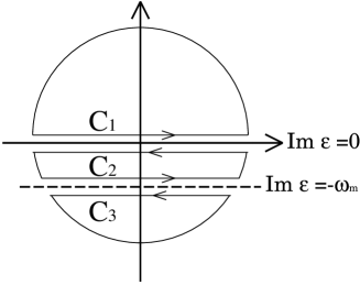
Figure 12: Contour to perform the sum over $\varepsilon_{n}$.

To evaluate $\chi^{R}_{d,{\rm RPA}}({\bm{q}},\omega)$, we need to calculate $\chi^{{\rm irr},R}_{d,0}({\bm{q}},\omega)$. On Matsubara (imaginary) axis, $\chi^{\rm irr}_{d,0}({\bm{q}},{\rm i}\omega_{m})$ is given by Eq. (38). We transform the Matsubara sum into an integral over the contour as shown in FIG. 12 using $T\sum_{\varepsilon_{n}}F({\rm i}\varepsilon_{n})=\oint\frac{d\varepsilon}{4\pi{\rm i}}\tanh(\frac{\varepsilon}{2T})F(\varepsilon)$, and perform analytical continuation ${\rm i}\omega_{m}\to\omega+{\rm i}0_{+}$. Contour ${\cal C}_{1}$ and ${\cal C}_{3}$ give the real part of $\chi^{R}_{d,0}({\bm{q}},\omega)$ for small $\omega$, and in this case we can evaluate this quantity in the limit $\omega\to 0$,

$${\rm Re}\chi^{{\rm irr},R}_{d,0}({\bm{q}},\omega) = \int\frac{d\varepsilon}{4\pi{\rm i}}\tanh\left(\frac{\varepsilon}{2T}\right)\int_{\bm{p}}d^{2}_{\bm{p}}$$ (64)

$$\times \Big{\{}\big{[}G_{\sigma^{*}}^{(0)R}({\bm{p}}+{\bm{q}},\varepsilon)G_{\sigma^{*}}^{(0)R}({\bm{p}},\varepsilon)\big{]}-c.c.\Big{\}}$$

$$= T\sum_{\varepsilon_{n}}\int_{\bm{p}}d^{2}_{\bm{p}}\big{[}G_{\sigma^{*}}^{(0)}({\bm{p}}+{\bm{q}},{\rm i}\varepsilon_{n})G_{\sigma^{*}}^{(0)}({\bm{p}},{\rm i}\varepsilon_{n})\big{]}$$

$$= \int_{\bm{p}}d^{2}_{\bm{p}}\bigg{\{}f{{}^{\prime}}_{\Gamma}(\xi_{{\bm{p}},\sigma^{*}})$$

$$+ \Big{[}\frac{f{{}^{\prime\prime}}_{\Gamma}(\xi_{{\bm{p}},\sigma^{*}})}{4}(M_{x}+M_{y})\Big{]}{\bm{q}}^{2}$$

$$+ \Big{[}\frac{f{{}^{\prime\prime\prime}}_{\Gamma}(\xi_{{\bm{p}},\sigma^{*}})}{12}(v_{x}^{2}+v_{y}^{2})\Big{]}{\bm{q}}^{2}\bigg{\}}+O({\bm{q}}^{4}),$$

where we have used $\frac{\partial}{\partial\xi_{\bm{p}}}G^{(0)}({\bm{p}},{\rm i}\varepsilon_{n})=[G^{(0)}({\bm{p}},{\rm i}\varepsilon_{n})]^{2}$ and $T\sum_{\varepsilon_{n}}[G^{(0)}_{\sigma}({\bm{p}},{\rm i}\varepsilon_{n})]^{n+1}=\frac{1}{n!}\frac{\partial^{n}}{\partial\xi_{{\bm{p}},\sigma}^{n}}f_{\Gamma}(\xi_{{\bm{p}},\sigma})$, and $M_{j}(j+x,y)$ is given below Eq. (42).

On the other hand, contour ${\cal C}_{2}$ gives the imaginary part of $\chi^{{\rm irr},R}_{d,0}({\bm{q}},\omega)$ for small $\omega\ll v_{\rm F}|{\bm{q}}|$ as

$${\rm Im}\chi^{{\rm irr},R}_{d,0}({\bm{q}},\omega) = -\int\frac{d\varepsilon}{4\pi{\rm i}}\int_{\bm{p}}d^{2}_{\bm{p}}\left(\frac{\tanh\left(\frac{\varepsilon}{2T}\right)}{{\rm i}/\tau-{\bm{v}}_{p}\cdot{\bm{q}}}\right)$$ (65)

$$\times \frac{\partial}{\partial\varepsilon}\big{[}G_{\sigma^{*}}^{(0)R}({\bm{p}},\varepsilon)-c.c.\big{]}\omega+O(\omega^{2})$$

$$= -T\sum_{\varepsilon_{n}}\int_{\bm{p}}d^{2}_{\bm{p}}\left(\frac{{\rm i}\omega}{2\Gamma+{\rm i}{\bm{v}}_{p}\cdot{\bm{q}}}\right)$$

$$\hskip 28.45274pt\times\frac{\partial}{\partial\xi_{\bm{p}}}G_{\sigma^{*}}^{(0)}({\bm{p}},{\rm i}\varepsilon_{n})+O(\omega^{2})$$

$$= \frac{{\rm i}\omega}{|{\bm{q}}|}\int_{\bm{p}}d^{2}_{\bm{p}}\left(\frac{-f{{}^{\prime}}_{\Gamma}(\xi_{{\bm{p}},\sigma^{*}})}{2\Gamma/|{\bm{q}}|+{\rm i}{\bm{v}}_{p}\cdot\widehat{{\bm{q}}}}\right)+O(\omega^{2}),$$

where we have used $\frac{\partial}{\partial\varepsilon}G_{\sigma}^{(0)R/A}({\bm{p}},\varepsilon)=-\frac{\partial}{\partial\xi_{\bm{p}}}G_{\sigma}^{(0)R/A}({\bm{p}},\varepsilon)$.

References

- (1) I. Pomeranchuk, Zh. Eksp. Teor. Fiz. 35, 524 (1958) [Sov. Phys. JETP 8, 361 (1959)].
- (2) V. Oganesyan, S. A. Kivelson, and E. Fradkin, Phys. Rev. B 64, 195109 (2001).
- (3) M. P. Lilly, K. B. Cooper, J. P. Eisenstein, L. N. Pfeiffer, and K. W. West, Phys. Rev. Lett. 82, 394 (1999).
- (4) H. Yamase and H. Kohno, J. Phys. Soc. Jpn. 69, 332 (2000).
- (5) C. J. Halboth and W. Metzner, Phys. Rev. Lett. 85, 5162 (2000).
- (6) V. Hankevych, I. Grote, and F. Wegner, Phys. Rev. B 66, 094516 (2002).
- (7) B. Valenzuela and M. A. H. Vozmediano, Phys. Rev. B 63, 153103 (2001).
- (8) C. Honerkamp, M. Salmhofer, and T. M. Rice, Eur. Phys. J. B 27, 127 (2002).
- (9) P. A. Frigeri, C. Honerkamp, and T. M. Rice, Eur. Phys. J. B 28, 61 (2002).
- (10) H.-Y. Kee, Phys. Rev. B 67, 073105 (2003).
- (11) H.-Y. Kee, E. H. Kim, and C.-H. Chung, Phys. Rev. B 68, 245109 (2003).
- (12) W. Metzner, D. Rohe, and S. Andergassen, Phys. Rev. Lett. 91, 066402 (2003).
- (13) A. Neumayr and W. Metzner, Phys. Rev. B 67, 035112 (2003).
- (14) H. Yamase, Phys. Rev. Lett. 93, 266404 (2004).
- (15) I. Khavkine, C.-H. Chung, V. Oganesyan, and H.-Y. Kee, Phys. Rev. B 70, 155110 (2004).
- (16) H-Y. Kee and Y. B. Kim, Phys. Rev. B 71, 184402 (2005).
- (17) H. Yamase, V. Oganesyan, and W. Metzner, Phys. Rev. B 72, 035114 (2005).
- (18) L. Dell’Anna and W. Metzner, Phys. Rev. B 73, 045127 (2006).
- (19) L. Dell’Anna and W. Metzner, Phys. Rev. Lett. 98, 136402 (2007).
- (20) P. Jakubczyk, P. Strack, A. A. Katanin, and W. Metzner, Phys. Rev. B 77, 195120 (2008).
- (21) S. A. Grigera, P. Gegenwart, R. A. Borzi, F. Weickert, A. J. Schofield, R. S. Perry, T. Tayama, T. Sakakibara, Y. Maeno, A. G. Green, and A. P. Mackenzie, Science 306, 1154 (2004).
- (22) R. A. Borzi, S. A. Grigera, J. Farrell, R. S. Perry, S. J. S. Lister, S. L. Lee, D. A. Tennant, Y. Maeno, and A. P. Mackenzie Science 315, 214 (2007).
- (23) V. Hinkov, S. Pailhés, P. Bourges, Y. Sidis, A. Ivanov, A. Kulakov, C. T. Lin, D. P. Chen, C. Bernhard, and B. Keimer, Nature 430, 650 (2004).
- (24) V. Hinkov, D. Haug, B. Fauqué P. Bourges, Y. Sidis, A. Ivanov, C. Bernhard, C. T. Lin, and B. Keimer, Science 319, 597 (2008) and references therein.
- (25) C. Xu, Y. Qi, and S. Sachdev, Phys. Rev. B 78, 134507 (2008).
- (26) H. Zhai, F. Wang, and D.-H Lee, arXiv:0905.1711v2.
- (27) J. E. Hirsch, Phys. Rev. B 41, 6820 (1990).
- (28) C. Wu and S. C. Zhang, Phys. Rev. Lett. 93, 036403 (2004).
- (29) C. Wu, K. Sun, E. Fradkin, and S. C. Zhang, Phys. Rev. B 75, 115103 (2007).
- (30) C. M. Varma and L. Zhu, Phys. Rev. Lett. 96, 036405 (2006).
- (31) H. Doh and H.-Y. Kee, Phys. Rev. B 75, 233102 (2007).
- (32) An example of using fluctuation effects to probe the symmetry of unconventional superconductors can be seen in V. J. Emery, J. Low Temp. Phys. 22, 467 (1976).
- (33) H. Adachi and R. Ikeda, J. Phys. Soc. Jpn, 70, 2848 (2001).
- (34) L. D. Landau and I. M. Khalatnikov, Dokl. Acad. Nauk SSSR, 96, 469 (1954).
- (35) T. Moriya, Spin fluctuations in Itinerant Electron Magnetism (Springer, Berlin, 1985).
- (36) H. Kleinert, Gauge Fields in Condensed Matter (World Scientific, 1989) Vol. 2, Chapter 7.
- (37) P. M. Chaikin and T. C. Lubensky, Principles of condensed matter physics (Cambridge, 1995) Chapter 7.
- (38) A. A. Abrikosov, L. E. Gor’kov and I. E. Dzyaloshinski, Methods of Quantum Field Theory in Statistical Physics (Prentice-Hall, N.J., 1963) Sect. 21.
- (39) R. H. Paulson and J. R. Schrieffer, Phys. Letters 27A, 289 (1968).
- (40) H.-Y. Kee, H. Doh, and T. Grzesiak, J. Phys.: Condens. Matter 20, 255248 (2008).
- (41) A. A. Nersesyan and G. E. Vachnadze, J. Low. Temp. Phys. 77, 293 (1989).
- (42) H. Yamase and A. A. Katanin, J. Phys. Soc. Jpn. 76, 073706 (2007).
- (43) A. F. Ho and A. J. Schofield, Eur. Phys. Lett. 84, 27007 (2008).
- (44) P. Fulde and A. Luther, Phys. Rev. 170, 570 (1968).
- (45) S. Hikami and T. Tsuneto, Prog. Theor. Phys. 63, 387 (1980).
- (46) H. Yamase, Phys. Rev. Lett. 102, 116404 (2009).
- (47) J. A. Hertz, Phys. Rev. B 14, 1165 (1976).
- (48) A. J. Millis, Phys. Rev. B 48, 7183 (1993).
- (49) A. Kawabata, J. Phys. F: Metal Phys. 4, 1477 (1974).
- (50) M. B. Walker, M. F. Smith, and K. V. Samokhin, Phys. Rev. B 65, 014517 (2001).
- (51) L. G. Aslamazov and A. I. Larkin, Phys. Lett. A 26, 238 (1968).
- (52) R. Ramazashvili and P. Coleman, Phys. Rev. Lett. 79, 3752 (1997).
- (53) K. Maki, Prog. Theor. Phys. 39, 897 (1968).
- (54) R. S. Thompson, Phys. Rev. B 1, 327 (1970).
- (55) E. Abrahams, M. Redi and J. W. F. Woo, Phys. Rev. B 1, 208 (1970).
- (56) B. Lüthi, T. J. Moran, and R. J. Pollina, J. Phys. Chem. Solids 31, 1741 (1970).
- (57) C. Honerkamp, Phys. Rev. B 72, 115103 (2005).
- (58) Ch. Puetter, H. Doh, and H.-Y. Kee, Phys. Rev. B 76, 235112 (2007).
- (59) R. S. Perry, L. M. Galvin, S. A. Grigera, L. Capogna, A. J. Schofield, A. P. Mackenzie, M. Chiao, S. R. Julian, S. I. Ikeda, S. Nakatsuji, Y. Maeno, and C. Pfleiderer, Phys. Rev. Lett. 86, 2661 (2001).
- (60) S. A. Grigera, R. S. Perry, A. J. Schofield, M. Chiao, S. R. Julian, G. G. Lonzarich, S. I. Ikeda, Y. Maeno, A. J. Millis, and A. P. Mackenzie, Science 294, 329 (2001).
- (61) A. J. Millis, A. J. Schofield, G. G. Lonzarich, and S. A. Grigera, Phys. Rev. Lett. 88, 217204 (2002).
- (62) B. Binz and M. Sigrist, Europhys. Lett. 65, 816 (2004).
- (63) E. Ohmichi, Y. Yoshida, S. I. Ikeda, N. V. Mushunikov, T. Goto, and T. Osada, Phys. Rev. B 67, 024432 (2003).
- (64) R. S. Perry, K. Kitagawa, S. A. Grigera, R. A. Borzi, A. P. Mackenzie, K. Ishida, and Y. Maeno, Phys. Rev. Lett. 92, 166602 (2004).
- (65) Z. X. Zhou, S. McCall, C. S. Alexander, J. E. Crow, P. Schlottmann, A. Bianchi, C. Capan, R. Movshovich, K. H. Kim, M. Jaime, N. Harrison, M. K. Haas, R. J. Cava, and G. Cao, Phys. Rev. B 69, 140409(R) (2004).
- (66) R. S. Perry, T. Tayama, K. Kitagawa, T. Sakakibara, K. Ishida, and Y. Maeno, J. Phys. Soc. Jpn. 74, 1270 (2005).
- (67) P. Gegenwart, F. Weickert, M. Garst, R. S. Perry, and Y. Maeno, Phys. Rev. Lett. 96, 136402 (2006).
- (68) K. Kitagawa, K. Ishida, R. S. Perry, T. Tayama, T. Sakakibara, and Y. Maeno, Phys. Rev. Lett. 95, 127001 (2005).
- (69) S. Raghu, A. Paramekanti, E-. A. Kim, R. A. Borzi, S. A. Grigera, A. P. Mackenzie, and S. A. Kivelson, Phys. Rev. B 79, 214402 (2009).
- (70) W.-C. Lee and C. Wu, arXiv: 0902.1337v1.
- (71) The form of the electron-phonon vertex should be changed if we start from and orbitals, but this does not change our conclusion.