Fast In-Memory XPath Search using Compressed Indexes

Abstract

A large fraction of an XML document typically consists of text data. The XPath query language allows to search such text via its equal, contains, and starts-with predicates. These predicates can be efficiently implemented using a compressed self-index of the document’s text data. Most queries, however, are hybrid: they contain parts which query the text of the document, and contain other parts which query the tree structure of the document. It is therefore a challenge to appropriately choose a query evaluation order which optimally leverages the execution speeds of the text and tree indexes. Here the SXSI system is introduced. It stores the tree structure of an XML document using a bit array of opening and closing brackets plus a sequence of labels, and stores the text nodes of the document using a global compressed self-index. On top of these indexes sits an XPath query engine that is based on tree automata. The engine uses fast counting queries on the text index in order to determine whether to evaluate top-down or bottom-up with respect to the tree structure. The resulting system has several advantages over existing systems: (1) on pure tree queries (without text search) such as the XPathMark queries, the SXSI system performs on par or better than the fastest known systems MonetDB and Qizx, and (2) on queries that use text search, SXSI outperforms the existing systems by 1–3 orders of magnitude (depending on the size of the result set), and (3) for all tested data and queries, SXSI’s memory consumption consistently stays below two times the document size.

1 Introduction

As more and more data is stored, transmitted, queried, and manipulated in XML, the popularity of XPath and XQuery as query languages for semi-structured data is increasing. Evaluating such XML queries efficiently is challenging, and has triggered much research. Today there is a wealth of public and commercial XPath/XQuery engines, apart from several theoretical proposals.

In this paper we focus on XPath, which is simpler and forms the basis of XQuery. XPath query engines can be roughly divided into two categories: sequential and indexed. In the former, which follows a streaming approach, no preprocessing of the XML data is performed. Each query sequentially reads the whole document, and the goal is to be as close as possible to making just one pass over the data, while using as little main memory as possible to hold intermediate results and data structures. Instead, the indexed approach preprocesses the XML document to build a data structure on it, so that later queries can be evaluated without traversing the whole document. A serious shortcoming of the indexed approach is that the index can use much more space than the original data, and thus may have to be manipulated on disk. There are two approaches for dealing with this problem: (1) to load the index only partially (by using clever clustering techniques), or (2) to use less powerful indexes which require less space. Examples of systems using these approaches are Qizx/DB quizx09 , MonetDB/XQuery bonea06 , and Tauro tauro .

In this work we aim at an index for XML that uses little space compared to the size of the data, so that the indexed document can fit in main memory for moderate-sized data, thereby solving XPath queries without any need of resorting to disk. An in-memory index should outperform streaming approaches, even when the data fits in RAM. This is confirmed when comparing our indexed approach against two well-known streaming XPath engines (over data coming from a RAM-disk): GCX DBLP:conf/vldb/KochSS07 and SPEX DBLP:journals/tkde/Olteanu07 run about $50$ and $350$ times, respectively, slower than our system. Of course such a comparison is hardly fair because the streaming engines need to parse the entire XML input document at each run.

Note that usually main memory XML query systems (such as Saxon kay08 , Galax ferea03 , Qizx/Open quizx09 , etc.) use machine pointers to represent XML data. We observe that on various well-established DOM implementations, this representation blows up memory consumption to about 5–10 times the size of the original XML document.

An XML document can be regarded essentially as a text collection (that is, a set of strings) organized into a tree structure, so that the strings correspond to the text data and the tree structure corresponds to the nesting of tags. The problem of manipulating text collections within compressed space is now well understood NM07 ; CHLS07 ; MN08 , and also much work has been carried out on compact data structures for trees Jacobson89 ; MunRam01 ; GearyRRR04 ; GRR04 ; BDMRRR05 ; DRR06 ; HMR07 ; FarMun08 ; Arr08 ; SN08 . In this paper we show how both types of compact data structures can be integrated into a compressed index representation for XML data, which is able to efficiently solve XPath queries.

A feature inherited from its components is that the compressed index replaces the XML document, in the sense that the data (or any part of it) can be efficiently reproduced from the index (and thus the data itself can be discarded). The result is called a self-index, as the data is inextricably tied to its index. A self-index for XML data was recently proposed FLMM05 ; FLMM06 , yet its support for XPath is reduced to a very limited class of queries that are handled particularly well. Namely, they handle “simple paths”, that is, queries of the form //$t_{1}$/$t_{2}$/ $\dots$ /$t_{k}$, where each $t_{i}$ is a tagname. For such queries they can count in time $O(k)$, and can report in time $O(\log^{1+\epsilon}n)$ per result. See DBLP:journals/corr/abs-1012-5696 where a comparison is presented which allows to conclude that, for result counting over XMark documents, their self-index can be between one and two orders of magnitude faster than our system.

The main value of our work is to provide the first practical and public tool for compressed indexing of XML data, dubbed Succinct XML Self-Index (SXSI), which takes little space, solves a significant portion of XPath, and largely outperforms the best public software supporting XPath we are aware of, namely MonetDB/XQuery bonea06 and Qizx/DB quizx09 . Currently we support at least forward Core XPath gotkocpic05 , i.e., all forward navigational axes, plus, additionally text() and the attribute axis, and the three text predicates $=$ (equality), contains, and starts-with. The main challenges in achieving our results have been to obtain practical implementations of compact data structures (for texts, trees, and others) that are at a theoretical stage, to develop new compact schemes tailored to this particular problem, and to develop query processing strategies tuned for the specific cost model that emerges from the use of these compact data structures. The limitations of our scheme are that it is in-memory, that it is static (i.e., the index must be rebuilt when the XML data changes), and that it does not handle XQuery. The first limitation is a design decision; the last two are subject of future work.

This paper introduces the three main ingredients of SXSI: (i) the text index, (ii) the tree index, and (iii) the query evaluator. While technical details on the first two components can be found elsewhere in the literature, we here only mention the main aspects of these components and focus on how they are integrated inside of the SXSI system. A new aspect of executing automata to solve XPath queries is the notion of relevant nodes xpathwhole ; intuitively, a node is relevant if the automaton must necessarily visit it to solve the query. A large speed-up is obtained by using the new “jump” primitives of our tree index in order to visit only relevant nodes. We present an algorithm for “true bottom-up runs”, which are beneficial if the query contains highly selective text predicates. In our experimental section we first test the core speeds of our indexes; for instance, timing global pattern counting over the text index against a naive string buffer, or, full traversals over the tree index against traversing a pointer-based tree store. The main part of the experimental section is about comparing SXSI against the state-of-the-art XPath engines MonetDB/XQuery and Qizx/DB. We use two batches of experiments: the “tree oriented” queries of the XPathMark benchmark DBLP:conf/xsym/Franceschet05 (over XMark data DBLP:conf/vldb/SchmidtWKCMB02 ) and our own “text oriented” queries (over Medline documents). Our results show that SXSI outperforms the other systems for virtually all tested queries, and moreover that the running times of SXSI are more predictable and “robust” than those of other systems.

2 Basic Concepts and Model

We regard an XML document as $(i)$ an ordered set of strings and $(ii)$ a labeled tree. The latter is the natural XML parse tree defined by the hierarchical tags, where the (normalized) tag name labels the corresponding node. We add an extra root node (labeled “&”) on top of the document’s root node; this node is needed for XPath semantics, but could also be used to hold additional information such as the document name. Each text node is represented as a leaf labeled #. Attributes are handled as follows in this model. Each node with attributes gets an additional single child labeled @ (at the first child position), and for each attribute @attr=value of the node, a child labeled attr is added to its @-node, and a leaf child labeled % to the attr-node. The text content value is then associated to that leaf. Therefore, there is exactly one string content associated to each tree leaf labeled # or %. We refer to those strings as texts. Note that we do not store empty texts; for instance, the XML document <a></a> is stored as a single a-labeled leaf node (which is the unique child of the $\&$-labeled root node).

Table 1: Notation.

Term	Meaning
$T$	Concatenation of all the texts in the collection
$u$	Length of $T$ in symbols
$\Sigma$	Alphabet of the distinct text symbols
$\sigma$	Size of $\Sigma$
$	Character that terminates each text in the collection
$n$	Number of nodes in the XML tree
$t$	Number of different tag and attribute names in the document
$d$	Number of texts in the XML tree (in our model, tree leaves)
$H_{k}(S)$	$k$-th order empirical entropy of string $S$

Let us call $T$ the set of all the texts and $u$ its total length measured in symbols, $n$ the total number of tree nodes, $\Sigma$ the alphabet of the strings and $\sigma=|\Sigma|$, $t$ the total number of different tag and attribute names, and $d$ the number of texts (or tree leaves). These receive text identifiers which are consecutive numbers assigned in a left-to-right parsing of the data. In our implementation $\Sigma$ is simply the set of byte values 1 to 255, and 0 will act as a special terminator called $\$$. This symbol occurs exactly once at the end of each text in $T$. Note that our implementation can easily support also UTF-8 encoding and hence adheres to the XML standard. Table 1 summarizes the notation.

To connect tree nodes and texts, we define global identifiers, which give unique numbers to both internal and leaf nodes, in depth-first preorder. Figure 1 shows a toy document (top left) and our model of it (top right), as well as its representation using our data structures (bottom), which serves as a running example for the rest of the paper. In the model, the tree is formed by the solid edges, whereas dotted edges display the connection with the set of texts. The tree contains the extra root node (labeled &), as well as extra internal nodes (labeled #, @, and %). Note how the attributes are handled. There are six texts, which are associated to the tree leaves and receive consecutive text numbers (marked in italics at their right). Global identifiers are associated to each node and leaf (drawn at their left). The conversion between tag names and symbols, drawn within the bottom-left component, is used to translate queries and to recreate the XML data. Note that if the return and space (indentation) characters are present precisely as shown in the “XML data” box of the figure, then there are indeed several additional #-leaves in the tree: for instance, the whitespace (return and space characters) after the initial <parts> and before the final </parts> give rise to two extra texts (and therefore the parts-node in the tree has additional first and last children labeled #). In total there are seven such whitespace texts which have been omitted in our figure for reasons of readability.

Figure 1: Our running example on representing an XML document.

Some notation and measures of compressibility follow, preceding a rough description of our space complexities. The empirical $k$-th order entropy Man01 of a sequence $S$ over alphabet $\Sigma$, $H_{k}(S)\leq\log\sigma$, is a lower bound to the output size per symbol of any $k$-th order compressor applied to $S$. The formula of the zero-order entropy is as follows:

$$H_{0}(S)=\sum_{c\in\Sigma}\frac{s_{c}}{s}\log\frac{s}{s_{c}},$$

where $s_{c}$ is the number of occurrences of $c$ in $S$ and $s=|S|$. We assume $\log=\log_{2}$ and $0\log 0=0$ henceforth. Let $\Sigma^{k}$ denote the set of words over $\Sigma$ of length $k$. Now let $S_{W}$ be the set of characters preceding the occurrences of $W\in\Sigma^{k}$ in $S$, then for $k>0$,

$$H_{k}(S)=\frac{1}{s}\sum_{W\in\Sigma^{k}}|S_{W}|H_{0}(S_{W}).$$

Note $0\leq H_{k}(S)\leq H_{k-1}(S)\leq\ldots\leq H_{0}(S)\leq\log\sigma$.

We will build on self-indexes able of handling text collections $T$ of total length $u$ within $uH_{k}(T)+o(u\log\sigma)$ bits NM07 ; FMMN07 ; MN08 . On the other hand, representing an unlabeled tree of $n$ nodes requires $2n-O(\log n)$ bits, and several representations using $2n+o(n)$ bits support many tree query and navigation operations in constant time (e.g., SN08 ). The labels require in principle other $n\log t$ bits. Sequences $S$ can be stored within $|S|\log\sigma(1+o(1))$ bits (and even $|S|H_{0}(S)+o(|S|\log\sigma)$), so that any element $S[i]$ can be accessed, and they can also efficiently answer the following queries GGV03 ; GMR06 ; FMMN07 :

$rank_{c}(S,i)$

is the number of $c$’s in $S[1,i]$;

$select_{c}(S,j)$

is the position of the $j$-th $c$ in $S$.

These are essential building blocks for more complex functionalities, as seen later.

The final space requirement of our index will include:

1. $uH_{k}(T)+o(u\log\sigma)$ bits for representing the text collection $T$ in self-indexed form. This supports the string searches of XPath and can (slowly) reproduce any text.

2. $d\log d+o(d\log d)$ bits for the mapping between the self-index and the text identifiers, e.g., to determine to which text identifier a self-index position belongs, or restricting self-index searches to some texts.

3. $2n+o(n)$ bits for representing the tree structure. This supports many navigational operations in constant time.

4. $4n\log t+2n+o(n)$ bits to represent the tags in a way that they support very fast XPath searches.

5. $2n+o(n)$ bits for mapping between tree nodes and text identifiers.

6. Optionally, $u\log\sigma$ or $uH_{k}(T)+o(u\log\sigma)$ bits, plus $O(d\log\frac{u}{d})$, to achieve faster text extraction than in 1).

As a practical yardstick, without the extra storage of texts (Item 6) the memory consumption of our system is about the size of the original XML file (and, being a self-index, includes it!), and with the extra text store the memory consumption is 1–2 times the size of the original XML file.

In Section 3 we describe our representation of the set of strings, including how to obtain text identifiers from text positions. This explains items 1, 2, and 6 above. Section 4 describes our representation for the tree and the labels, and the way the correspondence between tree nodes and text identifiers works. This explains items 3, 4, and 5. Section 5 describes how we process XPath queries on top of these compact data structures. In Sections LABEL:sec:imple and 6 we give some implementation details and empirically compare our SXSI engine with the most relevant public engines we are aware of. We conclude in Section 7.

3 Text Representation

Text data is represented as a succinct full-text self-index NM07 that is generally known as the FM-index FM05 . The index supports efficient pattern matching operations that can be easily extended to support different XPath predicates.

3.1 FM-Index and Backward Searching

Given a string $T$ of total length $u$, from an alphabet of size $\sigma$, the alphabet-friendly FM-index FMMN07 requires $uH_{k}(T)+o(u\log\sigma)$ bits of space. The index supports counting the number of occurrences of a pattern $P$ in $O(|P|\log\sigma)$ time. Locating the occurrences takes extra $O(\log^{1+\epsilon}u)$ time per answer, for any constant $\epsilon>1$.

The FM-index is based on the Burrows–Wheeler transform (BWT) of string $T$ BW94 . Assume $T$ ends with the special end-marker $\$$. Let $\mathcal{M}$ be a matrix whose rows are all the cyclic rotations of $T$ in lexicographic order. The first column of $\mathcal{M}$, denoted $F$, contains all symbols of $T$ in lexicographic order. The last column $L$ of $\mathcal{M}$ forms a permutation of $T$ which is the BWT string $L=T^{\text{\it bwt\/}}$. The matrix is only conceptual; the FM-index uses only on the $T^{\text{\it bwt\/}}$ string. Figure 2 illustrates the matrix $\mathcal{M}$ with its first and last rows ($F$ and $L=T^{\text{\it bwt\/}}$) in bold. Figure 1 (bottom right) shows how this fits in our overall scheme.

Figure 2: Example of the FM-index for text $T=\mathtt{``discontinued"}$ sampled each $l=3$ positions.

The resulting permutation from $T$ to $T^{\text{\it bwt\/}}$ is reversible. There exists a simple last-to-first mapping from symbols in $L$ to $F$ FM05 : Let $C[c]$ be the total number of symbols in $T$ that are lexicographically less than $c$. Then the LF-mapping is defined as

$$\text{\it LF\/}(i)=C[L[i]]+\text{\it rank}_{L[i]}(L,i).$$

Note that $L[i]$ is the symbol preceding the $i$-th lexicographically smallest row of $\mathcal{M}$. Thus, if $T^{\text{\it bwt\/}}[i]=T[j]$, then $T^{\text{\it bwt\/}}[\text{\it LF\/}(i)]=T[j-1]$. The symbols of $T$ can therefore be read in reverse order by starting from the location $i$ such that $T^{\text{\it bwt\/}}[i]=\$$, and applying LF recursively:

$T[u]=\$=T^{\text{\it bwt\/}}[i]$,
$T[u-1]=T^{\text{\it bwt\/}}[\text{\it LF\/}(i)]$,
$T[u-2]=T^{\text{\it bwt\/}}[\text{\it LF\/}(\text{\it LF\/}(i))]$,

and so on until, after $u$ steps, we get the first symbol $T[1]$. The values $C[c]$ can be stored in a small array of $\sigma\log u$ bits. Function $\text{\it rank}_{c}(L,i)$ can be computed in $O(\log\sigma)$ time with a data structure called wavelet tree which, when built on $T^{\text{\it bwt\/}}$, uses only $uH_{k}(T)+o(u\log\sigma)$ bits GGV03 ; FMMN07 . In practice we opt for a Huffman-shaped wavelet tree using uncompressed bitmaps inside CNspire08.1 . Despite this achieves space $u(H_{0}(T)+1)(1+o(1))$, it is much faster than the other implementations. In particular, operations cost $O(H_{0}(T))$ time on average, an improvement that applies to all the $O(\log\sigma)$ worst-case complexities that follow.

Pattern matching is supported via backward searching on the BWT FM05 . Given a pattern $P[1,m]$, the backward search starts with the range $[sp,ep]=[1,u]$ of rows in $\mathcal{M}$. At each step $i\in\{m,m-1,\ldots,1\}$ of the backward search, the range $[sp,ep]$ is updated to match all rows of $\mathcal{M}$ that have $P[i,m]$ as a prefix. New range $[sp^{\prime},ep^{\prime}]$ is given by $sp^{\prime}=C[P[i]]+\text{\it rank}_{P[i]}(L,sp-1)+1$ and $ep^{\prime}=C[P[i]]+\text{\it rank}_{P[i]}(L,ep)$. Each step takes $O(\log\sigma)$ time using the wavelet tree, and finally $ep-sp+1$ gives the number of times $P$ occurs in $T$. Figure 3 gives the pseudocode.

FM-Count($p_{1}p_{2}\ldots p_{m}$)
1.	$i:=m$
2.	$sp:=1$
3.	$ep:=n$
4.	While $sp\leq ep$ and $i\geq 1$ Do
5.		$c:=p_{i}$
6.		$sp:=C[c]+\text{\it rank}_{c}(T^{\text{\it bwt\/}},sp-1)+1$
7.		$ep:=C[c]+\text{\it rank}_{c}(T^{\text{\it bwt\/}},ep)$
8.		$i:=i-1$
9.	If $ep<sp$ Then
10.		Return $0$
11.	Else
12.		Return $ep-sp+1$

Figure 3: Counting on the FM-index.

To find out the location of each occurrence, the text is traversed backwards from each $sp\leq i\leq ep$ (virtually, using LF on $T^{\text{\it bwt\/}}$) until a sampled position is found. This is a sampling carried out at regular text positions, so that the corresponding positions in $T^{\text{\it bwt\/}}$ are marked in a bitmap $B_{s}[1,u]$, and the text position corresponding to $T^{\text{\it bwt\/}}[i]$, if $B_{s}[i]=1$, is stored in a samples array $P_{s}[\text{\it rank}_{1}(B_{s},i)]$. If every $l$-th position of $T$ is sampled, the extra space is $O((n/l)\log n)$ (including the compressed $B_{s}$ RRR02 ) and the locating takes $O(l\log\sigma)$ time per occurrence. Using $l=\Theta(\log^{1+\epsilon}u/\log\sigma)$ yields $o(u\log\sigma)$ extra space and locating time $O(\log^{1+\epsilon}u)$.

Figure 2 illustrates a sampling of $T$ each $l=3$ symbols. Assume we look for $P=\mathtt{``n"}$; then backward search finds $[sp,ep]=[8,9]$. Now to locate the occurrence at $8$ we see that $B_{s}[8]=0$, $B_{s}[\text{\it LF\/}(8)]=B_{s}[10]=0$, and finally $B_{s}[\text{\it LF\/}(10)]=B_{s}[2]=1$. This corresponds to position $P_{s}[\text{\it rank}_{1}(B_{s},2)]=P_{s}[2]=4$. Since we applied LF twice, the answer is $4+2=6$. We have found the occurrence $T[6..]=\mathtt{``n.."}$.

3.2 Text Collection and Queries

The textual content of the XML data is stored as $\$$-terminated strings so that each text corresponds to one string. Let $T$ be the concatenated sequence of the $d$ texts. Array $P_{s}$ is extended to record both the text identifier and the offset inside it. Since there are several $\$$’s in $T$, we fix a special ordering such that the end-marker of the $i$-th text appears at $F[i]$ in $\mathcal{M}$ (see Figure 1, bottom right). This generates a valid $T^{\text{\it bwt\/}}$ of all the texts and makes it easy to extract the $i$-th text starting from its $\$$-terminator.

Now $T^{\text{\it bwt\/}}$ contains all end-markers in some permuted order. This permutation is represented with a data structure Doc, that maps from positions of $s in $T^{\text{\it bwt\/}}$ to text identifiers. Let $T^{\text{\it bwt\/}}[j]$ correspond to the first symbol of the text with identifier $x$, thus if $i=\text{\it LF\/}(j)$ it holds $T^{\text{\it bwt\/}}[i]=\$$. Then we store $\text{\it Doc\/}[\text{\it rank}_{\$}(T^{\text{\it bwt\/}},i)]=x$. Furthermore, Doc can be stored in a format that allows for range searching (as illustrated in Figure 1 (right)): Given a range $[sp,ep]$ of $T^{\text{\it bwt\/}}$ and a range of text identifiers $[x,y]$, Doc can be used to output identifiers of all $\$$-terminators within the range $[sp,ep]\times[x,y]$, in $O(\log d)$ time per answer. In practice, because we only use the simpler functionality in the current system, Doc is implemented as a plain array using $d\log d$ bits.

Note Doc allows us to never switch from one text to another while looking for the preceding sampled value: If we reach a $ before finding any $B_{s}[i]=1$, array Doc can be used to determine that we are at the first position of some text with identifier $x$.

The basic pattern matching feature of the FM-index can be extended to support XPath functions such as starts-with, ends-with, contains, and operators $=$, $\leq$, $<$, $>$, $\geq$ for lexicographic ordering. Given a pattern and a range of text identifiers to be searched, these functions return all text identifiers that match the query within the range. In addition, existential (is there a match in the range?) and counting (how many matches in the range?) queries are supported. Time complexities are $O(|P|\log\sigma)$ for the search phase, plus an extra for reporting. While we describe the operators in their general form, which need the range reporting functionality from Doc, our current prototype implements only the simple case $[x,y]=[1,d]$, where Doc can be an array.

starts-with$(P,[x,y])$

:  The goal is to find texts in $[x,y]$ range prefixed by the given pattern $P$. After the normal backward search, the range $[sp,ep]$ in $T^{\text{\it bwt\/}}$ contains the end-markers of all the texts prefixed by $P$. Now $[sp,ep]\times[x,y]$ can be mapped to Doc, and existential and counting queries can be answered in $O(\log d)$ time. Matching text identifiers can be reported in $O(\log d)$ time per identifier.

ends-with$(P,[x,y])$

:  Backward searching is localized to texts in $[x,y]$ by choosing $[sp,ep]=[x,y]$ as the starting interval, since we have forced the ordering of $F[1,d]$ so that $F[z]=\$$ is the terminator of text with identifier $z$. After the backward search, the resulting range $[sp,ep]$ contains all possible matches, thus existential and counting queries are answered in constant time after the search. To find out text identifiers for each occurrence, the text must be traversed backwards to find a sampled position (or a $). The cost is $O(l\log\sigma)$ per answer, where $l$ is the sampling step.

operator $=(P,[x,y])$

:  Whole texts which are equal to $P$, and with identifiers in the range $[x,y]$, can be found as follows. Start with a backward search as in ends-with, and then map to the $\$$-terminators as in starts-with. The time complexities are same as in starts-with.

contains$(P,[x,y])$

: To find texts that contain $P$, we start with the normal backward search and finish like in ends-with. In this case there might be several occurrences inside one text, which have to be filtered. Thus, the time complexity is proportional to the total number of occurrences, $O(l\log\sigma)$ for each. Existential and counting queries are as slow as reporting queries. The basic $O(|P|\log\sigma)$-time counting of all the occurrences of $P$ can still be useful for query optimization.

operators $\leq$, $<$, $>$, $\geq$

: Operator $\leq$ matches texts that are lexicographically smaller than or equal to the given pattern. It can be solved like the starts-with query, but updating only the $ep$ of each backward search step, while $sp=1$ stays constant. While $[sp,ep]$ delimits the rows of $\mathcal{M}$ that start with $P[i,m]$, $[1,ep]$ delimits the rows that start with a prefix lexicographically smaller than or equal to $P[i,m]$. If at some point there are no occurrences of $P[i]=c$ within the prefix $L[1,ep]$, this means that $P[i,m]$ does not appear in $T$. To continue the search we replace $ep=C[c]$ and continue for $P[1,i-1]$. Other operators can be supported analogously, and costs are as for starts-with.

The new XPath extension, XPath Full Text 1.0 xqueryfulltext , suggests a wider selection of functionality for text searching. Implementation of these extensions requires regular expression and approximate searching functionalities, which can be supported within our index using the general backtracking framework Lametal08 : The idea is to alter the backward search to branch recursively to different ranges $[sp^{\prime},ep^{\prime}]$ representing the suffixes of the text prefixes (i.e., substrings). This is done by computing $sp_{c}^{\prime}=C[c]+\text{\it rank}_{c}(L,sp-1)+1$ and $ep_{c}^{\prime}=C[c]+\text{\it rank}_{c}(L,ep)$ for all $c\in\Sigma$ at each step and recursing on each $[sp_{c}^{\prime},ep_{c}^{\prime}]$. Then the pattern (or regular expression) can be compared with all substrings of the texts, allowing us to search for approximate occurrences Lametal08 . The running time becomes exponential in the number of errors allowed, but different branch-and-bound techniques can be used to obtain practical running times LTPS09 ; LD09 . We omit further details, as these extensions are out of the scope of this paper.

3.3 Construction and Text Extraction

The FM-index can be built by adapting any BWT construction algorithm. Linear time algorithms exist for the task, but their practical bottleneck is the peak memory consumption. Although there exist general time- and space-efficient construction algorithms, it turned out that our special case of text collection admits a tailored incremental BWT construction algorithm Sir09 (see the references and experimental comparison therein for previous work on BWT construction): The text collection is split into several smaller collections, and a temporary index is built for each of them separately. The temporary indexes are then merged, and finally converted into a static FM-index. The BWT allows extracting the $i$-th text by successively applying LF from $T^{\text{\it bwt\/}}[i]$, at $O(\log\sigma)$ cost per extracted symbol.

3.4 Additional Text Collections

To enable faster text extraction, we allow storing the texts in plain format in $n\log\sigma$ bits, or in an enhanced LZ78-compressed format (derived from the LZ-index ANS06 ) using $uH_{k}(T)+o(u\log\sigma)$ bits. These secondary text representations are coupled with a delta-encoded bit vector storing starting positions of each text in $T$. This bitmap requires $O(d\log\frac{u}{d})$ more bits.

In fact, keeping next to the FM-index an additional copy of all texts in plain format has more advantages. As mentioned before, the time complexity of contains-queries is proportional to the total number of occurrences. This implies that for large occurrence numbers, it becomes faster to search over the plain texts than over the FM-index. The precise cut-off point depends on the sampling factor $l$, see Section 6.3 for mor details. Since a global count over the FM-index is fast ($O(|P|\log\sigma)$ time), we use it to determine whether to search over the plain text or over the FM-index.

Since search over our implementaiton of the LZ-index is problematic, we only consider plain and FM-index from now on, and do not mention the LZ-index anymore.

4 Tree Representation

4.1 Data Representation

The tree structure of an XML collection is represented by the following compact data structures, which provide navigation and indexed access to it. See also the bottom left of Figure 1.

4.1.1 Par

This is the balanced parentheses representation of the tree structure (see, e.g., MR97 ). It is obtained by traversing the tree in depth-first-search (DFS) order, writing a "(" whenever we arrive at a node, and a ")" when we leave it (thus it is easily produced during the XML parsing). In this way, every node is represented by a pair of matching opening and closing parentheses. A tree node is identified by the position of its opening parenthesis in Par (that is, a node is just an integer index within Par). In particular, we use the balanced parentheses implementation of SN08 , which supports a very complete set of operations, including finding the $i$-th child of a node, in constant time; for more information concerning implementation details and performance, see DBLP:conf/alenex/ArroyueloCNS10 . Overall Par uses $2n+o(n)$ bits. This includes the space needed for constant-time binary rank on Par, which is very fast in practice.

4.1.2 Tag

This is the sequence of the tag identifiers of each tree node, including an opening and a closing version of each tag, to mark the beginning and ending point of each node. These tags are numbers in $[1,2t]$ and are aligned with Par so that the tag of node $i$ is simply $\textit{Tag\/}[i]$.

We also need rank and select queries on Tag. They allow to realize special operations such as “TaggedDesc” which “jumps” to the first descendant of the given node, such that the descendant has a given label (see Section 4.2.2). Several sequence representations supporting access and these operations are known GGV03 ; GMR06 ; CNspire08.1 . Given that Tag is not too critical in the overall space, but it is in time, we opt for a practical representation that favors speed over space. First, we store the tags in an array using $\lceil\log 2t\rceil$ bits per field, which gives constant time access to $\text{\it Tag}[i]$. The rank and select queries over the sequence of tags are answered by a second structure. Consider the binary matrix $R[1..2t][1..2n]$ such that $R[i,j]=1$ if $\textit{Tag\/}[j]=i$. We represent each row of the matrix using Okanohara and Sadakane’s structure sarray os07 . Its space requirement for each row $i$ is $n_{i}\log\frac{2n}{n_{i}}+n_{i}(2+o(1))$ bits, where $n_{i}$ is the number of times symbol $i$ appears in Tag. The total space of both structures adds up to $2n\log(2t)+2nH_{0}(\textit{Tag\/})+n(2+o(1))\leq 4n\log t+2n+o(n)$ bits. They support access and select in $O(1)$ time, and rank in $O(\log n)$ time.

4.2 Tree Navigation

We define the following operations over the tree structure, which are useful to support XPath queries over the tree. Most of these operations are supported in constant time, except when a rank over Tag is involved. Let $tag$ be a tag identifier.

4.2.1 Basic Tree Operations

These are direcly inherited from Sadakane’s implementation SN08 . We mention only the most important ones for this paper; $x$ is a node (a position in Par).

• Close$(x)$: The closing parenthesis matching $\text{\it Par\/}[x]$. If $x$ is a small subtree this takes a few local accesses to Par, otherwise a few non-local table accesses.

• Preorder$(x)=\text{\it rank\/}_{(}(\text{\it Par},i)$: Preorder number of $x$.

• SubtreeSize$(x)=(\textrm{Close}(x)-x+1)/2$: Number of nodes in the subtree rooted at $x$.

• IsAncestor$(x,y)=x\leq y\leq\textrm{Close}(x)$: Whether $x$ is an ancestor of $y$.

• FirstChild$(x)=x+1$: First child of $x$, if any.

• NextSibling$(x)=\textrm{Close}(x)+1$: Next sibling of $x$, if any.

• Parent$(x)$: Parent of $x$. Somewhat costlier than Close$(x)$ in practice, because the answer is less likely to be near $x$ in Par.

4.2.2 Connecting to Tags

The following operations are essential for our fast XPath evaluation.

• SubtreeTags$(x,\text{\it tag\/})$: Returns the number of occurrences of tag within the subtree rooted at node $x$. This is $\text{\it rank\/}_{\text{\it tag\/}}(\text{\it Tag},\textrm{Close}(x))-\text{\it rank\/}_{\text{\it tag\/}}(\text{\it Tag},x-1)$.

• Tag$(x)$: Gives the tag identifier of node $x$. In our representation this is just $\textit{Tag\/}[x]$.

• TaggedDesc$(x,\text{\it tag\/})$: The first node (in pre-order) labeled tag strictly within the subtree rooted at $x$. It is obtained as $select_{\text{\it tag\/}}(\text{\it Tag},$ $\text{\it rank\/}_{\text{\it tag\/}}(\text{\it Tag},x)+1)$ if it is $\leq\textrm{Close}(x)$, and undefined otherwise.

• TaggedPrec$(x,\text{\it tag\/})$: The last node labeled tag with preorder smaller than that of node $x$, and not an ancestor of $x$. Let $r=\text{\it rank\/}_{\text{\it tag\/}}(\text{\it Tag},x-1)$. If $select_{\text{\it tag\/}}(\text{\it Tag},r)$ is not an ancestor of node $x$, we stop. Otherwise, we set $r=r-1$ and iterate.

• TaggedFoll$(x,\text{\it tag\/})$: The first node labeled tag with preorder larger than that of $x$, and not in the subtree of $x$. This is $select_{\text{\it tag\/}}(\text{\it Tag},\text{\it rank\/}_{\text{\it tag\/}}(\text{\it Tag},\textrm{Close}(x))+1)$.

4.2.3 Connecting the Text and the Tree

Conversion between text numbers, tree nodes, and global identifiers, is easily carried out by using Par and a bitmap $B$ of $2n$ bits that marks the opening parentheses of tree leaves containing text, plus $o(n)$ extra bits to support rank/select queries; the latter uses an implementation of RRR02 which is described in CNspire08.1 . The bitmap $B$ enables the computation of the following operations:

• LeafNumber$(x)$: Gives the number of leaves up to $x$ in Par. This is $\text{\it rank\/}_{1}(B,x)$.

• TextIds$(x)$: Gives the range of text identifiers that descend from node $x$. This is simply $[\textrm{LeafNumber}(x-1)+1,\textrm{LeafNumber}(\textrm{Close}(x))]$.

• XMLIdText$(d)$: Gives the global identifier for the text with identifier $d$. This is Preorder$(select_{1}(B,d))$.

• XMLIdNode$(x)$: Gives the global identifier for a tree node $x$. This is just Preorder$(x)$.

4.3 Displaying Contents

Given a node $x$, we want to recreate its XML serialization, that is, return (a portion of) the original XML string. We traverse the structure starting from $\mbox{\it Par\/}[x]$, retrieving the tag names and the text contents, from the text identifiers. The time is $O(\log\sigma)$ per text symbol (or $O(1)$ if we use the redundant text storage described in Section 3) and $O(1)$ per tag.

• GetText$(d)$: Generates the text with identifier $d$.

• GetSubtree$(x)$: Generates the subtree at node $x$.

5 XPath Queries

Our goal is to support a practical subset of XPath, while being able to guarantee efficient evaluation based on the data structures described in the previous sections. As a first shot we target the forward fragment of “Core XPath” gotkocpic05 . We focus our presentation on the descendant and child axes, but self, attribute and following-sibling are also part of our implementation. Thus, the non-terminal “Axis” in the following EBNF can here be thought of as generating only the terminals “descendant” and “child”. A node test (non-terminal “NodeTest” below) is either the wildcard (“*”), a tag name, or a node type test, i.e., one of “text()” or “node()”. Note that our current prototype does not support the node type tests “comment()” and “processinginstruction()”. Of course, additional to Core XPath, we support all text predicates of XPath 1.0, i.e., the $=$, contains, and starts-with predicates. Here is an EBNF for Core XPath.

Core	::=	LocationPath $|$ ‘/’ LocationPath
LocationPath	::=	LocationStep (‘/’ LocationStep)*
LocationStep	::=	Axis ‘::’ NodeTest
		$|$ Axis ‘::’ NodeTest ‘[’ Pred ‘]’
Pred	::=	Pred ‘and’ Pred $|$ Pred ‘or’ Pred
		$|$ ‘not’ ‘(’ Pred ‘)’ $|$ Core $|$ ‘(’ Pred ‘)’

A data value is the value of an attribute or the content of a text node. Here, all data values are considered as strings. If an XPath expression selects only data values then we call it value expression. In our fragment, $p$ is a value expression if its last axis is the attribute axis or the text() test. Inside of a filter we call “self” (and “.”) a value expression if the last axis to the left of the filter is a value expression. Our XPath fragment (“Core+”), consists of Core XPath plus the following data value comparisons which may appear inside filters (that is, may be generated by the nonterminal Pred of above). Let $w$ be a string and $p$ a value expression.

• $p$ = $w$ (equality): tests if the string $w$ is equal to a string selected by $p$.

• contains$(p,w)$: tests if the string $w$ is contained in a string selected by $p$.

• starts-with$(p,w)$: tests if the string $w$ is a prefix of a string selected by $p$.

5.1 Tree Automata Representation

Tree automata are a well-known and popular tool for reasoning about XML, see, e.g., DBLP:journals/sigmod/Neven02 ; DBLP:journals/jcss/Schwentick07 ; DBLP:conf/icde/GenevesL10 ; DBLP:journals/japll/LibkinS10 . Only seldomly have they been used as a tool for query evaluation. In greenEA04 automata are used to evaluate, on an XML stream, many (very simple) XPath queries in parallel. It is well-known that Core XPath can be evaluated using tree automata; see, e.g., kochvldb03 and bjorklund09 . Here we use alternating tree automata (as in tata07 and haruo:book ). Such automata work with Boolean formulas over states, which must become satisfied for a transition to fire. This allows a much more compact representation of queries through automata, than ordinary tree automata (without formulas). Our tree automata are defined over a binary tree view of the XML tree where the left child is the first child of the XML node and the right child is the next sibling of the XML node.

Definition 1 (Non-deterministic marking automaton)

An automaton $\mathcal{A}$ is a tuple $(\mathcal{L},\mathcal{Q},\mathcal{T},\mathcal{B},\delta)$, where:

• $\mathcal{L}$ is a countable (possibly infinite) set of tree labels;

• $\mathcal{Q}$ is the finite set of states;

• $\mathcal{T}\subseteq\mathcal{Q}$ is the set of top states (that is, states that must be satisfied at the root node);

• $\mathcal{B}\subseteq\mathcal{Q}$ is the set of bottom states (that is, states that must be satisfied at the leaves);

• $\displaystyle\delta:\mathcal{Q}\times 2_{f}^{\mathcal{L}}\cup 2_{\textit{cof}}^{\mathcal{L}}\rightarrow F$ is the transition function, where $F$ is the set of Boolean formulas . A Boolean formula $\phi$ is a finite production of the grammar:

  $$\begin{array}[]{lcll}\phi&::=&\top~{}|~{}\bot~{}|~{}\phi\lor\phi~{}|~{}\phi\land\phi~{}|~{}\lnot\phi~{}|~{}a~{}|~{}p&\textrm{(formula)}\\ a&::=&\downarrow_{1}\!q~{}|~{}\downarrow_{2}\!q&\textrm{(atom)}\\ \end{array}$$

  where $p\in P$ is a built-in predicate and $q$ is a state.

Before explaining in details the use of formulas, we motivate our use of finite or co-finite sets as guards for transitions. While traditionally automata transitions are guarded by a state and a single label, this would make the encoding of XPath into automata very tedious and needlessly complicate the algorithms. Indeed, one of the features of XPath is a wildcard node test, namely “*”. One solution could be to suppose that for a given automaton the set of labels of the input document is known in advance and that this set is used as alphabet for the automaton. Unfortunately, this does not accurately reflect the semantics of XPath in which a query can be defined independently of any document and can even be executed on any document (it might not yield any result but its application is nonetheless valid). Another solution (as in greenEA04 ) is to equip automata with a special “default” transition, labelled for instance “_”, which is taken if in the current state no other transition can be evaluated. This has two drawbacks. Firstly, it is only well-defined for deterministic tree automata (our encoding makes heavy use of nondeterminism). Secondly, the evaluation function is polluted by the special cases which handle this default transition. Our solution is more blunt. We guard transitions by finite or co-finite sets of labels, and a transition is taken if the label of the current node is a member of that set. For instance, the “*” XPath test is encoded as a transition guarded by the set $\mathcal{L}-\{\text{@},\text{\#}\}$, where “@” and “#” represent labels of subtrees containing attribute nodes and text nodes in our encoding. This allows us to give a very straightforward evaluation function for tree automata, which relies on the evaluation of Boolean formulas, presented next.

Definition 2 (Evaluation of a formula)

Given an automaton $\mathcal{A}$ and an input tree $t$, the evaluation of a formula is given by the judgment $\mathcal{R}_{1},\mathcal{R}_{2},n\vdash_{\mathcal{A}}\phi=(b,R)$ where $\mathcal{R}_{1}$ and $\mathcal{R}_{2}$ are mappings from states to sets of nodes of $t$, $n$ is a node of $t$, $\phi$ is a formula, $b\in\{\top,\bot\}$, and $R$ is a set of nodes of $t$. We define the semantics of this judgment by the means of the inference rules given in Figure 4.

$$\begin{array}[]{c}\frac{\textrm{\footnotesize$$}}{\textrm{\footnotesize$\mathcal{R}_{1},\mathcal{R}_{2},t^{\prime}\vdash_{\mathcal{A}}\top=(\top,\emptyset)$}}\textbf{\small(true)}\\[10.0pt] \frac{\textrm{\footnotesize$\mathcal{R}_{1},\mathcal{R}_{2},t^{\prime}\vdash_{\mathcal{A}}\phi=(b,R)$}}{\textrm{\footnotesize$\mathcal{R}_{1},\mathcal{R}_{2},t^{\prime}\vdash_{\mathcal{A}}\lnot\phi=(\overline{b},\emptyset)$}}\textbf{\small(not)}\\[10.0pt] \frac{\textrm{\footnotesize$\begin{array}[]{c}\mathcal{R}_{1},\mathcal{R}_{2},t^{\prime}\vdash_{\mathcal{A}}\phi_{1}=(b_{1},R_{1})\\ \mathcal{R}_{1},\mathcal{R}_{2},t^{\prime}\vdash_{\mathcal{A}}\phi_{2}=(b_{2},R_{2})\\ \end{array}$}}{\textrm{\footnotesize$\mathcal{R}_{1},\mathcal{R}_{2},t^{\prime}\vdash_{\mathcal{A}}\phi_{1}\lor\phi_{2}=(b_{1},R_{1})\varovee(b_{2},R_{2})$}}\textbf{\small(or)}\\[10.0pt] \frac{\textrm{\footnotesize$\begin{array}[]{c}\mathcal{R}_{1},\mathcal{R}_{2},t^{\prime}\vdash_{\mathcal{A}}\phi_{1}=(b_{1},R_{1})\\ \mathcal{R}_{1},\mathcal{R}_{2},t^{\prime}\vdash_{\mathcal{A}}\phi_{2}=(b_{2},R_{2})\\ \end{array}$}}{\textrm{\footnotesize$\mathcal{R}_{1},\mathcal{R}_{2},t^{\prime}\vdash_{\mathcal{A}}\phi_{1}\land\phi_{2}=(b_{1},R_{1})\varowedge(b_{2},R_{2})$}}\textbf{\small(and)}\\[10.0pt] \frac{\textrm{\footnotesize$q\in\textrm{dom}(\mathcal{R}_{i})$}}{\textrm{\footnotesize$\mathcal{R}_{1},\mathcal{R}_{2},t^{\prime}\vdash_{\mathcal{A}}\downarrow_{i}\!q=(\top,\mathcal{R}(q))$}}\text{\small for~{}$i\in\{1,2\}$}~{}\textbf{\small(left,right)}\\[10.0pt] \frac{\textrm{\footnotesize$$}}{\textrm{\footnotesize$\mathcal{R}_{1},\mathcal{R}_{2},t^{\prime}\vdash_{\mathcal{A}}\texttt{mark}=(\top,\{t^{\prime}\})$}}\textbf{\small(mark)}\\[14.22636pt] \frac{\textrm{\footnotesize$EvalPred($p$,$t'$)=$b, R$$}}{\textrm{\footnotesize$\mathcal{R}_{1},\mathcal{R}_{2},t^{\prime}\vdash_{\mathcal{A}}p=(b,R)$}}\textbf{\small(pred)}\\[10.0pt] \frac{\textrm{\footnotesize$\textrm{when no other rule applies}$}}{\textrm{\footnotesize$\mathcal{R}_{1},\mathcal{R}_{2},t^{\prime}\vdash_{\mathcal{A}}\phi=(\bot,\emptyset)$}}\end{array}$$

where:

$$\begin{array}[]{l}\overline{\top}=\bot\quad\text{ and }\quad\overline{\bot}=\top\\ (b_{1},R_{1})\ovee(b_{2},R_{2})=\left\{\small\begin{array}[]{cr}\top,R_{1}&\textrm{if $b_{1}=\top$, $b_{2}=\bot$}\\ \top,R_{2}&\textrm{if $b_{2}=\top$, $b_{1}=\bot$}\\ \top,R_{1}\cup R_{2}&\textrm{if $b_{1}=\top$, $b_{2}=\top$}\\ \bot,\emptyset&\textrm{otherwise}\\ \end{array}\right.\\[10.0pt] (b_{1},R_{1})\owedge(b_{2},R_{2})=\left\{\small\begin{array}[]{cr}\top,R_{1}\cup R_{2}&\textrm{if $b_{1}=\top$, $b_{2}=\top$}\\ \bot,\emptyset&\textrm{otherwise}\\ \end{array}\right.\end{array}$$

Figure 4: Inference rules defining the evaluation of a formula

These rules are straightforward and combine the rules for a classical alternating automaton, with the rules of a marking automaton. Rules (or) and (and) implements the Boolean connective of the formula and collect the marking found in their true sub-formulas. Rules (left) and (right) (written as a rule schema for concision) evaluate to true if the state $q$ is in the corresponding set. Intuitively, $\mathcal{R}_{1}$ (resp. $\mathcal{R}_{2}$) is the set of states recognizing the left (resp. right) subtree of the input tree. Rule (pred) supposes the existence of an evaluation function for built-in predicates. Among the latter, we suppose the existence of a special predicate mark, which evaluates to $\top$ and returns the singleton set containing the current node.

We now give the semantics of an automaton by means of the run function TopDownRun (see Figure 5).

TopDownRun($\mathcal{A}$, $t$, $r$)
1.	If $t$ is the empty tree Then
2.		Return $\{q\rightarrow\varnothing\mid q\in\mathcal{B}\cap r\}$
3.	Else
4.		$\textit{trans}:=\{q,\ell\,\rightarrow\phi\mid q\in r\textrm{~{}and~{}}\textrm{Tag}(t)\in\ell\}$
5.		$r_{i}:=\{q\mid\downarrow_{i}\!q\in\phi,\forall\phi\in\textit{trans}\}$,  for $i\in\{1,2\}$
6.		$\mathcal{R}_{1}:=\textbf{TopDownRun}(\mathcal{A},\textrm{FirstChild}(t),r_{1})$
7.		$\mathcal{R}_{2}:=\textbf{TopDownRun}(\mathcal{A},\textrm{NextSibling}(t),r_{2})$
8.		Return $\displaystyle\bigcup_{~{}~{}~{}~{}(q,\ell\rightarrow\phi)\in\textit{trans}}\{q\mapsto R\mid\mathcal{R}_{1},\mathcal{R}_{2},t\vdash_{\mathcal{A}},\phi=(\top,R)\}$

Figure 5: Evaluation function for tree automata

This algorithm is based on the text book algorithm for recursive bottom-up evaluation of tree automata (see e.g. haruo:book ). The algorithm performs a recursive first child/next sibling traversal of the tree until a leaf is reached (base case for the recursion). When returning form the recursive evaluation on the left and right subtrees (Lines 6 and 7, Figure5) the function evaluate the set of transitions for the current node, based on the set of states recognizing the left and right subtree. However, instead of blindly doing a recursive descent from the root to the leaves and evaluating when returning from the recursive calls, the transitions are restricted by the set of states $r$ (Line 4). This technique is dubbed “bottom-up evaluation with top-down preprocessing” in haruo:book . We therefore named the run function TopDownRun to differentiate it from a real bottom-up run (starting from the leaves of the tree) that we present in Section 5.3.2. The novelty is our use of maps from states to nodes instead of only sets of states, to efficiently implement the marking of selected nodes.

5.2 From XPath to Automata

The translation of an XPath query to an alternating automaton is a simple syntax-directed translation which can be carried out in one pass through the parse tree of the query. Roughly speaking, the resulting automaton is “isomorphic” to the original query (and has essentially the same size). We illustrate the translation by an example. Consider the query

$$\texttt{/descendant::listitem/descendant::keyword[}\\ \texttt{emph]}$$

for which the automaton is

$$\mathcal{A}=(\mathcal{L},\{q_{0},q_{1},q_{2}\},\{q_{0}\},\{q_{1},q_{2}\},\delta)$$

where $\delta$ contains the following transitions (recall that &, @, and # denote the special tags for the document node, attribute nodes, and text nodes, respectively):

$$\begin{array}[]{l|@{\hspace{3pt}}lcl}1\hfil\lx@intercol\vrule\hskip 3.0&q_{0},\{\text{\&}\}&\rightarrow&\downarrow_{1}\!q_{1}\\[2.84526pt] 2\hfil\lx@intercol\vrule\hskip 3.0&q_{1},\{\mbox{{listitem}}\}&\rightarrow&\downarrow_{1}\!q_{2}~{}\land~{}\downarrow_{1}\!q_{1}~{}\land~{}\downarrow_{2}\!q_{1}\\ 3\hfil\lx@intercol\vrule\hskip 3.0&q_{1},\mathcal{L}-\{\text{@},\text{\#}\}&\rightarrow&\downarrow_{1}\!q_{1}~{}\land~{}\downarrow_{2}\!q_{1}\\[2.84526pt] 4\hfil\lx@intercol\vrule\hskip 3.0&q_{2},\{\mbox{{keyword}}\}&\rightarrow&\texttt{mark}~{}\land~{}\downarrow_{1}\!q_{3}~{}\land~{}\downarrow_{1}\!q_{2}~{}\land~{}\downarrow_{2}\!q_{2}\\ 5\hfil\lx@intercol\vrule\hskip 3.0&q_{2},\mathcal{L}-\{\text{@},\text{\#}\}&\rightarrow&\downarrow_{1}\!q_{2}~{}\land~{}\downarrow_{2}\!q_{2}\\[2.84526pt] 6\hfil\lx@intercol\vrule\hskip 3.0&q_{3},\{\mbox{{emph}}\}&\rightarrow&\top\\ 7\hfil\lx@intercol\vrule\hskip 3.0&q_{3},\mathcal{L}-\{\text{@},\text{\#}\}&\rightarrow&\downarrow_{2}\!q_{3}\\ \end{array}$$

It is clear that this encoding is linear in the size of the query. For each step, we create one state and two transitions. The first transition (Transitions 2, 4, and 6 above) represents the action the automaton performs when the current node matches the step at issue. For instance if Transition 2 is taken, it means that the current node has label listitem and that:

• the state encoding the rest of the query, namely $q_{2}$, recognizes the left subtree (hence the $\downarrow_{1}\!q_{2}$)

• the current step also holds recursively for the descendant and following nodes of the current node (because of $\downarrow_{1}\!q_{1}\land\downarrow_{2}\!q_{1}$).

The second transition associated with a step handles the default case and the recursion. For instance, in Transition 3, if the current node is not a listitem  or if it is a listitem for which the continuation path does not hold, then we just stay in the same states for descendant and following nodes. This use of non-determinism (since $\{\texttt{listitem}\}\subseteq\mathcal{L}-\{\text{@},\text{\#}\}$) is crucial to keep the automaton linear in the size of the query. Lastly, note how “top-level steps” (listitem and keyword in our example) are encoded by universal transitions, in which the use of the “$\land$” connectives forces the formula to be recursively checked down to the leaves (and therefore explores the tree to find all occurrences of such steps) while “filter steps” (here emph) are encoded as existential transitions, which become satisfied as soon as one node verifies them.

5.3 Leveraging the Speed of the Low-Level Interface

We have seen how to evaluate an XPath query by compiling it into a tree automaton and running the latter on the input document. We present now several techniques that make use of the tree and text index presented in Sections 4 and 3. It is these techniques that make our SXSI prototype competitive in speed with state-of-the-art XML databases.

5.3.1 Jumping to relevant nodes

Conventionally, the run of a tree automaton visits every node of the input tree. This is for instance the behaviour of the tree automata presented in kochvldb03 , which perform two scans of the whole XML document (the latter being stored on disk in a particular format). However, for typical queries, most of the nodes are “useless” in the sense that the automaton only loops through them staying in the same set of states. In other words, the automaton ignores most of the nodes. To restrict the run to interesting nodes, we use the notion of relevant nodes introduced in xpathwhole . While the full characterization is out of the scope of this paper, we give a flavor of relevant nodes, using an example. Consider the query

/descendant::listitem/descendant::keyword

Clearly, we only care about listitem and keyword and how they are positioned with respect to each other. This is precisely the information that is provided through the TaggedDesc and TaggedFoll functions of the tree representation. These functions allow us to have a “contracted” view of the tree, restricted to nodes with certain labels of interest (but preserving the overall tree structure). For instance, to solve the above query we can call TaggedDesc(Root, listitem) which selects the first listitem node $x$. Now, simply traverse recursively the subtree rooted at $x$, using TaggedDesc(_, keyword) and TaggedFoll(_, keyword) instead of FirstChild and NextSibling. After this, we determine the next listitem node using TaggedFoll($x$, listitem). We do this optimization of “jumping run” based on the automaton: for a given set of states of the automaton we compute the set of relevant transitions which cause a state change. The labels of those transitions are the relevant labels to which we jump, using TaggedDesc and TaggedFoll. For instance, in the automaton for the above query (which is the same as the one given in Section 5.2, minus state $q_{3}$ and corresponding transitions) only Transitions 2 and 4 are relevant (that is, these transitions are valid only when the automaton is on a relevant node). Thus, in state $q_{0}$ the automaton can use TaggedDesc to jump to listitem nodes, and in state $q_{1}$ it can jump to keyword nodes. It should be noted that for such a query, our “jumping run” is optimal: the automaton only visits the top-most listitem nodes and all the keyword nodes below them. This behaviour is similar to the idea of “partitioning and pruning” in the staircase join grukeuteu03 , but here achieved by means of automata.

5.3.2 Bottom-Up Runs

While the previous technique works well for tree-based queries it still remains slow for very selective value-based queries. For instance, consider the query

//listitem//keyword[contains(.,"Unique")]

The text interface described in Section 3 can answer the text predicate very efficiently returning the set of text nodes matching this contains query. If the number of occurrences is low, and in particular smaller than the number of listitem or keyword tags in the document (which can also be determined efficiently through the tree structure interface), then it would be faster to take these text nodes as starting point for query evaluation and test if their path upward to the root matches the XPath expression //listitem//keyword. This scheme is particularly useful for text oriented queries with low selectivity text predicates. However, it also applies for tree only queries: imagine the query //listitem//keyword on a tree with many listitem nodes but only a few keyword nodes. We can start bottom-up by jumping to the keyword nodes and then check their ancestors for listitem nodes. (Note that with the tree index described here, we cannot directly jump to all bottom-most keyword nodes. We would need to iterate through all keyword nodes. Direct access could be provided through additional sarrays storing for each label its bottom-most nodes.)

We now devise a real bottom-up evaluation algorithm of our automata. The algorithm takes an automaton and a sequence of potential match nodes (in our example, the text nodes containing the string "Unique"). It then moves up to the root, using the Parent function and checks that the automaton arrives at the root node in its initial state $q_{i}$. Note that, if naively done, such a bottom-up run will visit many nodes repeatedly: if a node is the common-ancestor of $m$ potential match nodes, then it would be visited $m$ times.

Instead, we move bottom-up left-to-right, and only move upwards from the left-most potential match until we reach its lowest common ancestor with the next potential match. This technique is similar in spirit to shift-reduce parsing (see compilers ). This scheme is illustrated in Figure 6.

(a) Initial TopDownRun
(b) MatchAbove walks upwards and ignores non-matching subtrees

(a) MatchAbove stops at the common ancestor of $t_{1}$ and $t_{2}$
(b) Recursive call on $t_{2}$, climbs up to $t^{\prime}_{1}$

Results of left and right subtrees are merged at $t^{\prime}_{1}$ and the initial MatchAbove restarts

Figure 6: Illustration of the bottom-up run

Consider a sequence [$t_{1}$,…,$t_{n}$] (ordered in pre-order) of potentially matching nodes. The algorithm starts on node $t_{1}$. First, if the node is not a leaf, we call the TopDownRun function on $t_{1}$ with $r=\mathcal{Q}$. This returns the mapping $\mathcal{R}_{1}$ of all states accepting $t_{1}$. We move from $t_{1}$ upwards to the document root, starting with states $\textrm{dom}(\mathcal{R}_{1})$. Once we arrive at a node $t^{\prime}_{1}$ which is an ancestor of the next potential matching subtree $t_{2}$, we stop at $t^{\prime}_{1}$ and start the algorithm on $t_{2}$ until it reaches $t^{\prime}_{1}$. Upon reaching $t^{\prime}_{1}$, we merge both mappings and continue upwards until we reach the root or a common ancestor of $t^{\prime}_{1}$ and $t_{3}$, and so on. The idea of “stopping” at a node to explore the the next potential matching subtree is similar to the shift action of a bottom-up parser: the stopped node is pushed onto a stack (here the recursive call stack) while the rest of the symbols are processed. Similarly, the “merging” of two nodes which are then replaced by their lowest common ancestor is similar to the reduce action of a bottom-up parser: two symbols are removed from the parsing stack and replaced by the non-terminal of the corresponding grammar rule. Merging the runs at the lowest common ancestor guaranties that we never touch any node more than once, during a bottom-up run. The bottom-up run algorithm is given in Figure 7.

BottomUpRun($\mathcal{A}$, $s$)
1.	If $s$ is empty Then
2.		Return $\varnothing$
3.	Else
4.		$t_{1},s^{\prime}:=\text{Head(s)},\text{Tail(s)}$
5.		$\mathcal{R}:=\textbf{TopDownRun}(\mathcal{A},t_{1},\mathcal{Q})$
6.		$\mathcal{R}^{\prime},s^{\prime\prime}:=\textbf{MatchAbove}(\mathcal{A},t,s^{\prime},\mathcal{R},\#)$
7.		Return $\mathcal{R}^{\prime}$
MatchAbove($\mathcal{A}$, $t$, $s$, $\mathcal{R}_{1}$, stop)
8.	If $t$ = stop Then
9.		Return $\mathcal{R}_{1},s$
10.	Else
11.		$p:=\textrm{Parent}(t)$
12.		If $s$ is empty or not(IsAncestor($p$, $t_{2}$)) Then
13.			$\mathcal{R}_{2},s^{\prime\prime}:=\varnothing,s$
14.		Else
15.			$t_{2},s^{\prime}:=\text{Head(s)},\text{Tail(s)}$
16.			$\mathcal{R}:=\textbf{TopDownRun}(\mathcal{A},t_{2},\mathcal{Q})$
17.			$\mathcal{R}_{2},s^{\prime\prime}:=\textbf{MatchAbove}(\mathcal{A},t_{2},s^{\prime},\mathcal{R},p)$
18.		$\textit{trans}:=\{q,\ell\rightarrow\phi\mid\begin{array}[]{l}\exists q^{\prime}\in\textrm{dom}(\mathcal{R}_{i})s.t.\downarrow_{i}\!q^{\prime}\in\phi\\ \textrm{Tag}(p)\in\ell\end{array}\}$
19.		$\displaystyle\mathcal{R}^{\prime}:=\bigcup_{~{}~{}~{}(q,\ell\rightarrow\phi)\in\textit{trans}}\{q\mapsto R\mid\mathcal{R}_{1},\mathcal{R}_{2},t\vdash_{\mathcal{A}},\phi=(\top,R)\}$
20.		Return MatchAbove($\mathcal{A}$, $p$, $s^{\prime}$, $\mathcal{R}^{\prime}$, stop)

Figure 7: Bottom-up evaluation function

The first function takes an automaton and a sequence of potential matches in pre-order, and proceed to run the automaton bottom-up from the left-most potential match ($t_{1}$, Line 6, Figure 7). The MatchAbove function is the one “climbing-up” the tree. We assume that the Parent$(\_)$ function returns the empty tree when applied to the root node. If the input node is not equal to the sentinel stop node (which is initially the empty tree #, allowing to stop only after the root node has been processed) then we first check whether the next potential match is a descendant of our parent (Line 12). If so, then we pause for the current branch and recursively call MatchAbove with our parent as stop tree. Once it returns, we compute all the possible transitions that the automata can take from the parent node to arrive on the left and right subtree with the correct configuration (Line 18). We then merge both configurations using the same computation as in the top-down algorithm (Line 19). Finally, we recursively call MatchAbove on the parent node, with the new configuration and sequence of potential matching nodes (Line 20).

5.4 General Optimizations, On-the-fly Determinization

While the optimizations presented in the previous sections give the most important speed-up we describe hereafter a series of implementation techniques used for the efficient evaluation of automata.

5.4.1 Hash consing of data-structures

We use hash consing for all critical data-structures: sets of states, formulas, sets of transitions, sets of labels and so on. Hash consed values have the following two properties. First, structurally equal values are shared in memory. Therefore testing for equality of such values (for instance testing that two sets of transitions are equal) consists in comparing their memory address (which is cheap). Second, to each such value we can associate a unique integer id (this can be its memory address for instance but more interestingly a small integer assigned at the creation of the value). These two properties —especially the second one— are instrumental to the other optimizations. Indeed, as described in ConchonFilliatre06 , we can memoize (or cache) the results of expensive computations and reuse them when needed instead of recomputing them. In particular, we can associate to each function a table, indexed by the the argument’s id. While the first computation might be expensive, its result is stored once and for all in the table and can be retrieved with one pointer indirection later on, when the same computation is requested. We explain now how this generic technique comes into play for automata evaluation.

5.4.2 Just-in-time compilation of automata

In the TopDownRun algorithm (Figure 5) the most expensive operations are in Lines 4, 5, and 8. By expensive we mean that they take time $O(|Q|)$ where $|Q|$ is the number of steps in the original query. At Line 4, we gather all the transitions that can be selected from the current label $\ell$ and set of states $r$. From these we compute, at Line 5, the new set of states $r_{1}$ and $r_{2}$ onto which we will launch the recursive call. As explained in Section 5.3, from the set of states $r_{1}$ (resp. $r_{2}$) we compute the “jump” moves that the automaton will do to reach the next node in the left (resp. right) subtree. If none of the formulas requires the evaluation of a value predicate (such as contains for instance) then we can see that this whole computation of Lines 4 and 5 can be cached in a 2-dimensional array, using only $\ell$ (the current label, identified by a small integer) and $r$ (a hash consed set of states with a unique small id) as key. In practice we store in this table a small sequence of instructions that are computed at run time and which represent the behaviour of the automaton for the next step (for instance “jump to the next keyword label in state $\{q_{0},q_{1}\}$). This just-in-time compilation scheme absorbs in practice most of the overhead caused by the automaton machinery and makes running an automaton almost as fast as executing a hand-written, precompiled function. In the same fashion, the computation of the judgment $\vdash_{\mathcal{A}}$ can be memoized, this time in two parts. First, the sets of states (that is the domain of the resulting mapping) is simply stored once and for all, and second, a sequence of instructions telling how to propagate the results from the left and right subtrees is stored and evaluated for each node.

5.4.3 Handling of result sets

Maintaining sets of (result) nodes can be expensive. Our efficient management of sets of nodes relies on the following two observations. First, note that only the states outside of filters actually accumulate nodes. All other states always yield empty bindings. Thus we can split the set of states into marking and regular states. This reduces the number of $\ovee$ and $\owedge$ operations on result sets. Note also that given a transition $q_{i},\ell\rightarrow\downarrow_{1}\!q_{j}\land\downarrow_{2}\!q_{k}$ where $q_{i}$, $q_{j}$, and $q_{k}$ are marking states, all nodes accumulated in $q_{j}$ are in the left subtree of the current node. Likewise, all the nodes accumulated in $q_{k}$ are subtrees of the right subtree of the current node. Thus both sets of nodes are disjoint and we do not need to keep sorted sets of nodes but only need sequences which support $O(1)$ concatenation. Computing the union of two result sets $R_{j}$ and $R_{k}$ can therefore be done in constant time and consequently $\ovee$ and $\owedge$ can be implemented in constant time.

5.4.4 Lazy result sets

Another way to leverage the speed and jumping capabilities of our tree index is by making use of a lazy result set. Consider the query //listitem//keyword. When reaching a listitem node, the automaton is in a state which encodes the following behaviour: “accumulate all keyword nodes below this node”. Therefore instead of having the automaton jump through the subtree to individually put each keyword node in the result set, we only store the listitem node (i.e. the current node during evaluation) and a flag to remember that during serialization, it is not the listitem node which should be printed but rather all its keyword descendants. Since our tree index allows us to reach each such node using a constant time jump operation, we delay the process of getting all the final result nodes until serialization, therefore speeding up the materialization process. This not only saves time but also memory since the full set of nodes do not have to by materialized in memory.

5.4.5 Early evaluation of formulas

Another optimization consists in evaluating the Boolean formulas of the automaton as early as possible. First, remark that in the TopDownRun algorithm, a node is “visited” three times. Once when the automaton enters the node, during the top-down phase (Line 1). Here, we only know that at most all states in $r$ yield a successful run. Then when returning from the left subtree (Line 6), we know $\mathcal{R}_{1}$ that is, the states which yield an accepting run for the left subtree. The idea now is to perform a partial evaluation of formulas using only $\mathcal{R}_{1}$. If this happens to be sufficient to prove or disprove the states in $r$, then the right subtree can be skipped altogether. This optimization is very important for filters as it insures that for instance in a query such as //listitem[.//keyword] the run function only tests for the presence of the left-most keyword node below a listitem node.

5.4.6 Relative Tag position tables

As explained earlier, the transitions for the query

…/descendant::keyword/…

would be (just-in-time) compiled into a piece of code performing a subtree traversal using TaggedDesc(_ , keyword) and TaggedFoll(_ , keyword) instead of FirstChild and NextSibling. This is already optimal for documents where keyword nodes may appear arbitrarily. However, it is often the case that labels are not recursive (that is, nodes with a label $l$ do not occur below other $l$-labelled nodes). To further optimize the compilation of the automaton, we build –while indexing the document– four relative position tables, telling for each label $l$ in the document the sets of labels that occur respectively in child position, descendant position, following-sibling position and following position. When compiling at runtime the automaton and generating a call to TaggedDescendant for a label $l$, we check that this $l$ label can indeed appear as descendant of the label of the current node (and similarly for other jumping functions). If the label does not occur, then the TaggedDescendant call is replaced by a constant function returning directly the correct sets of states for the left subtree as well as an empty result set, as if the automaton had made a full-run on this subtree and found nothing.

6 Experimental Results

This section presents our experimental results and is organized as follows. We first describe our experimental settings, test machines, and benchmark data. We then provide a first round of experiments illustrating the raw performances of the tree and text index: indexing time and resulting index size, performing full pre-order traversal using FirstChild and NextSibling moves, and direct querying of the text index. A third subsection illustrates how the tree index and automata-based engine work together to achieve very fast tree-oriented query evaluation (in particular using the jumping moves described in Section 4.1.2). We then show how the automaton machinery can leverage the speed of both the text and tree index by evaluating queries containing both text and tree predicates. Lastly we illustrate the versatility of our approach: our engine is easily extended to support querying of XML document storing bio-genetic data.

We have implemented a prototype XPath evaluator based on the data structures and algorithms presented in the previous sections. Both the tree structure and the FM-index were developed in C++, while the XPath engine was written using the OCaml language.

6.1 Protocol

To validate our approach we benchmark our implementation against two well established XQuery implementations, MonetDB/XQuery and Qizx/DB. We describe our experimental settings hereafter.

Test machine

Our test machine features an Intel Core i5 platform featuring 3.33Ghz cores, 3.8 GB of RAM and a S-ATA hard drive. The OS is a 64-bit version of Ubuntu Linux (11.04). The kernel version is 2.6.38 and the file system used to store the various files is ext4, with default settings. All tests are run on a minimal environment where only the tested program and essential services were running. We use the standard compiler and libraries available on this distribution (namely g++ 4.6.1, libxml2 2.7.8 for document parsing and OCaml 3.11.2).

Qizx/DB

We use version 3.0 of Qizx/DB engine (free edition), running on top of the 64-bit version of the JVM (with the -server flag set as recommended in the Qizx user manual). The maximal amount of memory of the JVM is set to the maximal amount of physical memory (using the -Xmx flag). We also use the flag -r of the Qizx/DB command line interface, which allows us to re-run the same query without restarting the whole program (this ensures that the JVM’s garbage collector and thread machinery do not impact the performances). We use the timing provided by Qizx debugging flags, and report the serialization time (which actually includes the materialization of the results in memory and the serialization).

MonetDB/XQuery

We use version Oct2010-SP1 of MonetDB, and in particular, version 4.40.3 of MonetDB4 server and version 0.40.3 of the XQuery module (pathfinder). We use the timing reported by the “-t” flag of MonetDB client program, mclient. We keep the materialization time and the serialization time separate.

Running times and memory reporting

For each query, we keep the best of five runs. For Qizx/DB, each individual run consists of two repeated runs (“-r 2”), the second one being always faster. For MonetDB, before each batch of five runs, the server is exited properly and restarted. For all systems, we exclude from the running times the time used for loading the index into main memory (based on the engines’ timing reports). We monitor the resident set size of each process which corresponds to the amount of process memory actually mapped in physical memory.

For the tests in which serialization is involved we serialize to the /dev/null device (that is, all the results are discarded without causing any output operation).

Remarks

We also compared with Tauro tauro . Yet, as it uses a tailored query language, we could not produce comparable results.

6.2 Indexing

Our implementation features a versatile index. It is divided into three parts. First, the tree representation composed of the parenthesis structure, as well as the tag structure. Second, the FM-index encoding the text collection. Third, the auxiliary text representation allowing fast extraction of text content.

It is easy to determine from the query which parts of the index are needed in order to solve it, and thus load only those into main memory. For instance, if a query only involves tree navigation, then having the FM-index in memory is unnecessary. On the other hand, if we are interested in very selective text-oriented queries, then only the tree part and FM-index are needed (both for counting and serializing the results). In this case, serialization is a bit slower (due to the cost of text extraction from the FM-index) but remains acceptable since the number of results is low; see Table 2 for a comparison of the serialization speed of the FM-index versus serializing from plain string buffers in memory.

Figure 8 reports the construction time and memory consumption of the indexing process, the loading time from disk into main memory of a constructed index, and a comparison between the size of the original document and the size of our in-memory structures.

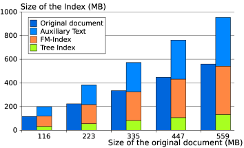
Document Size (MB) 116 223 335 447 559 Index construction time (min) 5’1 10’40 17’ 23’ 29’40 Index construction mem. use (MB) 296 568 844 1085 1387 Index loading time (s) 0.5 1.5 2.0 2.4 2.5

Figure 8: Indexing of XMark documents

For these indexes, a sampling factor $l=64$ (cf. Section 3) was chosen. It should be noted that the size of the tree index plus the size of the FM-index is always less than the size of the original document.

It should further be noted that although loading time is acceptable, it dominates query answering time. This is however not a problem for the use case we have targeted: a main memory query engine where the same large document is queried many times. As mentioned in the Introduction, systems such as MonetDB load their indexes only partially; this gives superior performance in a cold-cache scenario when compared with our system.

6.3 Raw Performance of Text Index

	GlobalCount		ContainsCount		Report-	mem
q	number	time	number	time	Contains	(MB)
1	1	.004	1	0.04	0.012	61
2	22	.009	19	2.281	1.588	61
3	392	.009	144	29.924	32.668	61
4	438	.009	438	4.616	4.457	61
5	1472	.008	966	128.28	122.014	61
6	2685	.005	1493	218.462	215.196	61
7	6897	.005	4690	553.496	548.009	62
8	10402	.005	8534	401.214	399.674	62
9	20859	.004	12073	1722.95	1717.83	62
10	63332	.004	22974	5084.14	5083.77	63
11	238638	.003	42586	19641.8	19630.3	64
12	2932251	.001	595716	189299	188377	93
13	9730750	.001	5870474	132780	132241	86

(q1, …, q13) = ( “Bakst”, “ruminants”, “morphine”, “AUSTRALIA”, “molecule”, “brain”, “human”, “blood”, “from”, “with”, “in”, “a”, “$\backslash$n”)

Table 2: Search times of FM-index (in ms), sampling factor $l=64$

	GlobalCount		ContainsCount		Contains-	mem
q	number	time	number	time	Report	(MB)
1	1	.005	1	0.049	0.013	100
2	22	.01	19	0.156	0.086	100
3	392	..009	144	1.718	1.357	100
4	438	.009	438	4.145	3.942	100
5	1472	.009	966	6.247	5.853	101
6	2685	.006	1493	12.24	11.588	101
7	6897	.005	4690	25.403	27.344	101
8	10402	.005	8534	77.175	73.613	101
9	20859	.003	12073	84.012	78.663	101
10	63332	.004	22974	242.834	235.043	102
11	238638	.002	42586	1105.6	1091.43	103
12	411409	.001	135307	1779.27	1762.62	108
13	748326	.001	320440	3411.65	3378.85	119
14	2932251	001	595716	13183.4	13173.4	133
15	9730750	.001	5870474	87770.9	88230.4	126

(q1, …, q15) = ( “Bakst”, “ruminants”, “morphine”, “AUSTRALIA”, “molecule”, “brain”, “human”, “blood”, “from”, “with”, “in”, “b”, “g”, “a”, “$\backslash$n”)

Table 3: Search times of FM-index (in ms), sampling factor $l=4$

Here we give a short overview of the performance of our implementation of the FM-index. We present the search times for different versions of contains-queries:

1. $\text{\it GlobalCount\/}(P)$: returns the global number of occurrences of the pattern $P$ in all texts.

2. $\text{\it ContainsCount\/}(P)$: returns the number of texts that contain $P$,

3. $\text{\it ContainsReport\/}(P)$: returns the positions of all occurrences of $P$ in the texts.

Our experiments are over the text collection obtained from a 116MB XMark XML document DBLP:conf/vldb/SchmidtWKCMB02 . The size of this text is around 82MB (if stored in one-byte per character ASCII format). Our “plain” alternative to the FM-index is a naive (byte-wise) string buffer (using precisely 82MB of memory). To search over the plain buffer, we use OCaml’s regular string expression library. The naive search time is constant for all our queries at around $2700$ms. For both the naive and the FM-index, the result positions ($32$ bit integers) for ContainsReport queries are materialized in an array. Consider now the performance of our FM-index in comparison. First at sampling factor $l=64$, shown in Table 2. As can be seen, the times for ContainsCount and ContainsReport for the word “from” are at around $1720$ms. Thus, in this case it is still faster to search over the FM-index. On the other hand, for the word “with” the search time is over $5000$ms, thus, here the plain search becomes faster. Hence, somewhere between $20859$ and $63332$ occurrences lies the cut-off point from which on searching over the plain text is faster than over the FM-index. Table 3 shows timings obtained with sampling factor $l=4$. As can be seen the cut-off point is now much later, at a global count somewhere between $411409$ and $748326$. The last columns of Tables 2 and 3 show the maximal memory consumption for these queries over the FM-index. As mentioned in the beginning of this section, we measure the maximum memory used by the process, as report by the operating system( this is a slight over-approximation of the actual memory). The memory overhead for queries with large cardinality, such as the last queries (q13 and q15), is explained by the size of the result array: for both sampling factors this is around 25MB. This query has around 6 million results (ContainsCount-number), each result is stored as a 4 Byte integer. Thus, 23MB are needed. However, additional memory overhead occurs when results are removed from the GlobalCount (because they occur in the same XML text node). For instance, in the second to last query (q12/q14) the ratio of GlobalCount-number to ContainsCount-number is much larger than for the last query ($4.9$ versus $1.7$); it means that on average there are around $5$ “a”-characters per text node, while there are only around $1.7$ return-characters per text node. Correspondingly, the maximum memory consumption is much higher too.

6.4 Raw Performance of Tree Index

file	parse	pointer	parent	tag	tag-tabs
XMark116M	89446	373	504	4682	1324
XMark223M	220143	716	976	9051	2544
XMark559M	620479	7923	2415	22857	6283
Treebank83M	67412	465	615	14067	18867
medline122M	67935	537	760	6933	2036

Table 4: Construction times in ms for pointer versus SXSI tree store

The performance of some low-level features of our tree index is compared with the corresponding performance of a standard pointer-based implementation of a tree. The latter provides for each tree node two 64-bit pointers to its first child and next sibling nodes (and does not store labels). We first compare construction times. Then we compare times for a full depth-first left-to-right tree traversal on the different structures. Finally, we test the speed of the taggedDesc and taggedFoll functions. We compare different traversals through all nodes with a given label: (i) using a pure C++ function, (ii) using our automata in counting mode, and (iii) using our automata in materialization mode.

Construction

As Table 4 shows, the construction of the parenthesis structure takes roughly $1.5$-times the amount of time of allocation a pointer structure for the tree. Constructing the tag sequence is considerable slower, about ten times as much as building the parenthesis structure. This is because for each opening and for each closing tag, a separate sarray is constructed (see bottom left of Figure 1). The last column shows the time for building the four tag-to-tag tables described in Section 5.4.6. We also show the XML parsing time in the first column of the table.

Full Traversals

	recursive, all nodes			element nodes, SXSI
file	#nod	pointer	SXSI	#nod	rec.	//*
XMark116M	6	33	109	1.7	71	153
XMark223M	12	63	209	3.3	137	296
XMark559M	30	164	535	8.4	345	756
Treebank83M	7	57	184	2.4	136	292
medline122M	9	48	164	2.9	112	244

Table 5: Traversal times (in ms), #nodes (in millions)

The left part of Table 5 shows that a full tree traversal through all nodes is between $3.2$ and $3.4$ times slower with SXSI, than with a pointer tree data structure. Note that the pointers are allocated in pre-order too giving optimal performance for pre-order traversal. As a comparison, if the pointers are allocated in post-order, then traversal time for the pr-order traversal is almost twice as slow as the numbers reported, and if pointers are allocated in in-order, then the times are a bit over twice as slow; see DBLP:conf/alenex/ArroyueloCNS10 for a discussion of the phenomenon. It should also be noted that for other access patterns, such as random root-to-leaf traversals, the time difference between pointer and succinct trees is much larger, factors of up to $100$ are measure in DBLP:conf/alenex/ArroyueloCNS10 .

In the right part of Table 5 we see the number of element nodes in these trees, and the time it takes for SXSI to recurse through those node: either using a small recursive C-function (column “rec.”), or using the automaton for the XPath query //*, and executing in counting mode.

Tagged Traversals

tag	#nodes	jump(C++)	//(cou)	//(mat)
category	1040	1.2	1.6	1.7
price	10141	2.3	2.9	3.1
listitem	63179	16	22	24
keyword	73070	11	12	14

Table 6: Iteration through all tag-labeled nodes over XMark116M

Here the speed of the TaggedDesc and TaggedFoll functions is investigated. Using these two functions, three different traversal through all nodes with a given label are considered: first, by a small C++ function, and second and third by our automata through a //label query in counting and materializing modes, respectively. For instance, Table 6 shows that iterating through all keyword-nodes of the 116MB Xmark document takes essentially the same time for all three methods (11–14ms). This is in contrast to some other labels: for listitem for instance, the count-automaton traversal is $1.5$-times slower than the C++ traversal. This can be explained by the fact that listitem is a recursive tag: there are in fact 23298 listitem nodes that appear as descendants of listitem nodes. Hence, at each listitem node the automaton issues a taggedDescendant to search for further nodes. The other labels such as keyword and category do not appear recursively. Since this information is part of our tree index (cf. Section 5.4.6), the automaton run function avoids all these taggedDesc calls, which brings the speed almost up to the one of the C++ function.

6.5 XPath Tree Queries

We benchmark tree queries using the queries given in Figure 9.

Q01	/site/regions
Q02	/site/regions/*/item
Q03	/site/closed_auctions/closed_auction
	/annotation/description/text/keyword
Q04	//listitem//keyword
Q05	/site/closed_auctions/closed_auction[
	annotation/description/text/keyword]/date
Q06	/site/closed_auctions/closed_auction[ .//keyword]/date
Q07	/site/people/person[ profile/gender and profile/age]/name
Q08	/site/people/person[ phone or homepage]/name
Q09	/site/people/person[ address and (phone or homepage) and
	(creditcard or profile)]/name
Q10	//listitem[not(.//keyword/emph)]//parlist
Q11	//listitem[ (.//keyword or .//emph) and
	(.//emph or .//bold)]/parlist
Q12	//people[ .//person[not(address)] and
	.//person[not(watches)]]/person[watches]
Q13	/*[ .//* ]
Q14	//*
Q15	//*//*
Q16	//*//*//*
Q17	//*//*//*//*

Figure 9: Tree oriented queries

Queries Q01 to Q12 are taken from the XPathMark benchmark fra07 , derived from the XMark XQuery benchmark suite. Q13 to Q17 are “crash tests” that are either simple (Q13 selects only the root since it always has at least one descendant in our files) or generate roughly the same amount of results but with various intermediate result sizes.

Query answering time

For this experiment we use XMark documents of size 116MB and 1GB. In the cases of MonetDB and Qizx, the files were indexed using the default settings. Let us describe in detail Figure 10. Each of the six graphs should be read as follows. For each query (Q1 to Q17), the graph reports as vertical bars the relative running time of the three engines with respect to SXSI’s running time (therefore SXSI’s score is always 100%). In these graphs a higher bar means that the engine was slower. We also give at the top of each bar the average running time for the query in millisecond (or seconds, if the number is suffixed with an “s”). For instance, in the first graph —labelled “116 MB (counting)”— we can see that for query Q1, SXSI evaluates the query in 1.3ms, MonetDB 6.8ms (or roughly 500% of SXSI’s speed) and QizX 3.5 ms (or roughly 275% of SXSI’s speed). For count queries, the timing for all three engines are given side by side (SXSI, MonetDB and QizX in that order). For full reporting queries however, we want to gauge precisely the amount of time spent during materialization and during serialization. The definition of materialization seems to fit both MonetDB and SXSI: create a data-structure in memory which holds the resulting nodes in order and without duplicates such that access of the first result in pre-order can be done in constant time, and accessing the next resulting node in pre-order can also be done in constant time. The timing for both SXSI and MonetDB are given in the graphs labelled “(materialization)”. As we explained earlier, QizX interleaves evaluation of the query and serialization, therefore we only compared it to SXSI and MonetDB in the “(materialization+serialization)” series. We also checked that all three engines generated in the end the same amount of data while in serialization mode and that they generated valid XML documents (in particular, characters such as “&” were escaped correctly).

116MB (counting)

116MB (materialization)

116MB (mat. + serialization)

1GB (counting)

1GB (materialization)

1GB (mat. + serialization)

 SXSI query time   SXSI serialization time   MonetDB query time   MonetDB serialization time   Qizx query time   Qizx query + serialization time
+++ : query could not be run or took more than 15 minutes

Figure 10: Running times for the tree based queries (in milliseconds or seconds and as percent of SXSI’s speed. Lower bars are better.)

From the results of Figure 10, we see how the different components of SXSI contribute to the efficient evaluation model. Fully qualified paths, such as queries Q1–3 and Q5 illustrate the sheer speed of the tree structure and in particular the efficiency of its basic operations (such as FirstChild and NextSibling, which are used for the child axis), as well as the efficient execution scheme provided by the automaton. The descendant axes (used e.g. in Q4, Q6, Q10–12) show the impact of the jumping primitives and the computation of relevant nodes. Complex filters (Q6–12) show how the alternating automata can efficiently evaluate complex Boolean formulas corresponding to structural conditions over subtrees of a given node, including negations of paths.

Finally, Q12 to Q16 illustrate the robustness of our automata model. Indeed while such queries might seem unrealistic, the good performances that we obtain are the combination of (i) using an automata based evaluator (which factors in the states of the automaton all the necessary computation and thus do not materialize unneeded intermediate results) and (ii) our implementation of lazy result sets, which shifts the burden of walking through the document as much as possible to the serialization process.

Memory use and precision

While it is straightforward to predict the memory consumption of our engine with respect to the index part (the full index is mapped in memory excluding the Auxiliary Text, see Figure 8), the behaviour of the automaton evaluation function is unclear. Indeed, to speed-up the computation we create memoization tables, we handle partial result sets, and we perform recursive procedures which might be as deep as the binary encoding of the XML document (since we recurse on FirstChild and NextSibling move) thus increasing the size of the call stack.

Figure 11: Memory use in MB for XMark 116MB documents (excluding the index)

We report in Figure 11 the memory consumption for the automata evalutation of materialization queries. This includes the size of the recursive call stack, the size of OCaml’s heap (which is grown dynamically by OCaml’s garbage collector to accomadate the memory need). On the heap are allocated the memoization tables, intermediary structures and final result sets. As one can see, the memory use is very modest, peaking at 32 MB for query Q11. While we do not compare directly with MonetDB or QizX for memory consumption (since these engines try to max out the memory use to achieve better speed) we see that we can reach comparable (if not greater) speed while being very conservative memory wise.

To gauge the precision of our automata based approach, we report in Figure 12 for each query:

• the number of visited nodes (that is, the number of nodes that are given as argument to the top_down_run function);

• the number of marked nodes (that is, the number of nodes that considered as potential results at some point during evaluation);

• and finally the number of result nodes for the query.

A first observation is that the number of marked nodes is almost always the same as the number of result nodes (save for query Q5–10). This shows that using automata and early evaluation of Boolean formulas, we can decide early during query evaluation whether a node is indeed a result or not. Another point of interest is that for several queries (Q2, Q4, Q14–17) we only visit result nodes. While it might be expected for queries Q14–17 for which virtually every node is a result, queries such as Q2 or Q4 are very selective. However, these queries provide enough information for the runtime analysis of relevant nodes to be exact and therefore only touch result nodes. In general of course, the number of traversed node is larger than the number of resulting nodes but always far less than the whole document. Queries Q14 to Q17 show the impact of lazy result sets where we mark several nodes (whole subtrees actually) in one function call, and therefore manage to return more nodes than we have actually visited.

Figure 12: Comparison of visited, marked and result nodes for each query (logarithmic scale)

Lastly, we can see that the shapes of the “Visited Nodes” curve in Figure 12 and the memory use (Figure 11) are quite similar (the former being flattened by the logarithmic scale). This (quite expectedly) show that the number of visited nodes (and not the number of result nodes or intermediary results) impacts directly the memory consumption of our query engine.

6.6 XPath Text Queries

We tested the text capabilities of our XPath engine against the most advanced text oriented features of other query engines.

Qizx/DB

We use the newly introduced Full-Text extension of XQuery available in Qizx/DB v. 3.0. We try to formulate the queries as efficiently as possible while preserving the semantics of our original queries. The query used always gave better results than its pure XPath counterpart. In particular, we use the ftcontains text predicate xqueryfulltext implemented by Qizx/DB. The ftcontains predicate allows to express not only contains-like queries but also Boolean operations on text predicates, regular expression matching and so on. It is more efficient than the standard contains.

MonetDB

MonetDB supports some full-text capabilities through the use of the PF/Tijah text index pftija . However, this index only supports a complex about operator, which returns approximate matches and ranks results by order of relevance. Since about queries returned very different results than standard contains one, we did not include them but rather used the standard (and un-optimized) fn:contains functions from the XPath standard library. Interestingly, while these text functions are unoptimized, they sometimes outperform QizX/DB’s full-text implementation. However, the reader should keep in mind that MonetDB’s timing are given only for reference and are not used here as a direct comparison (since they implement the full semantics of fn:contains itself relying on fn:string conversions as defined in the XPath specification, they are bound to be slower than the full-text alternative).

Experiments are made on a 122MB Medline file. This file contains bibliographic information about life sciences and biomedical publications. This test file features 5,732,159 text elements, for a total amount of 95MB of text content. Figure 13 shows the text queries that we test.

			Query running time in ms
		# results	S Text	S Auto	S Total	Q	M
T1	//Article[ .//AbstractText[ contains ( . , "plus") ] ]	358	3.1	2.8	5.9	41.2	224
T2	//Article[ .//AbstractText[ contains ( . , "brain") ] ]	1104	5.2	9.0	14.2	69.5	420
T3	//Article[ .//Year[ . = "1997" ] ]	1237	2.2	8.7	10.9	48	230
T4	//MedlineCitation/Article/AuthorList/Author[ LastName[starts-with( . , "Bar")]]	630	2.24	0.25	2.5	111.25	167.85
T5	//*[ .//LastName[ contains( . , "Nguyen") ] ]	154	1.9	0.4	2.3	765	1433
T6	//*//*[ contains( . , "epididymis") ]	88	2.0	0.2	2.2	1221	5218
T7	//*[ .//PublicationType[ ends-with( . , "Article") ]]	81187	29.3	170.7	200	438	1531
T8	//MedlineCitation[ .//Country[ . = "AUSTRALIA" ]]	326	2.0	2.6	4.6	38	54

S Text: SXSI’s text collection   S Auto: SXSI’s Automata query engine   S Total: Total running time for SXSI
Q: total running time for Qizx/DB   M: total running time for MonetDB/XQuery

Figure 13: Text oriented queries

We use count queries for all three engines. The table in Figure 13 summarizes the running times for each query. As we target very selective text queries, we also give, for each query, the number of results it returned. Since for these queries our automata worked in “bottom-up” mode, we detail the two following operations:

• Calling the text predicate globally on the text collection, thus retrieving all the probable matches of the query (S Text column in the table of Figure 13)

• Running the automaton bottom up from the set of probable matches to keep those satisfying the path expression (S Auto in the table of Figure 13)

As it is clear from the experiments, the bottom-up strategy pays off. The only down-side of this approach is that the automaton uses Parent moves, which are less efficient than FirstChild and NextSibling. This can be seen in query T7 where the increase in the number of results makes the relative slowness of the automata more visible. However our evaluator still outperforms the other engines even in this case.

6.7 Biological Sequence Queries

As a last experiment, we demonstrate the versatility of SXSI by showing that it can be used as a very efficient Biological database, answering queries which make use of both the tree structure and a tailored text index. More precisely, we create XML files that combine gene annotations with their DNA sequences. A sample DTD for these files is given in Figure 14.

<!ELEMENT  chromosome  (name, gene*) >
<!ELEMENT  name        #PCDATA >
<!ELEMENT  gene        (name, strand, biotype, status,
      description?, promoter, sequence, transcript*) >
<!ELEMENT  strand      #PCDATA >
<!ELEMENT  biotype     #PCDATA >
<!ELEMENT  status      #PCDATA >
<!ELEMENT  description #PCDATA >
<!ELEMENT  promoter    #PCDATA >
<!ELEMENT  sequence    #PCDATA >
<!ELEMENT  transcript  (name, start, end, exon*,
                        sequence, protein?) >
<!ELEMENT  start       #PCDATA >
<!ELEMENT  end         #PCDATA >
<!ELEMENT  exon        (name, start, end, sequence) >

Figure 14: DTD for bio-genetic data

In this DTD, the elements promoter and sequence are of particular interest: they store the DNA represented as long sequences of A, T, C, G characters. The other #PCDATA elements store the gene annotation data such as positions, names and so on.

Our experiment data is composed from human chromosome five which contains 2719 genes having in total 8330 different transcripts. For each gene, we include 1000 base pairs of its upstream promoter sequence, the gene sequence itself (all exons and introns included), and annotation information such as gene’s biotype and description. Additionally, we include all known transcripts of each gene, that is, sequences of the exons they contain as well as the concatenation of these exons. The resulting textual content is highly repetitive since each one of the exon sequences can appear in many transcripts. Highly repetitive data has been shown to compress well using certain run-length encoded text-indexes Maekinen2010 , thus, here the text-index implementation is switched to use RLCSA Maekinen2010 instead of the FM-index. In this example, the final XML file is 132 MB while the text-index requires only 63 MB of memory plus 59 MB for the samples array. The full index, including tree and text, is around 135 MB, that is only as big as the original document. The resulting XML document contains 323318 elements of which 65286 are either promoter or sequence nodes containing genetic data.

To do biologically relevant XML queries, we extend our engine to support PSSM queries (Position Specific Scoring Matrix) which allows to search for transcription factor binding sites from genes’ promoter regions. Input for this query is an Position Frequency Matrix (PFM) and a minimum threshold for a valid match. The matrices can be found from e.g. the Jaspar database jaspar.

In a nutshell, PFM’s have one row for each symbol of the alphabet (in our case 4 rows A, T, C, G) and one column for each position in the pattern to search. For instance, the PFM:

$$\left[\begin{array}[]{ccccc}A&0&20&10&1\\ T&30&10&0&0\\ C&0&0&10&20\\ G&18&6&6&6\\ \end{array}\right]$$

denotes patterns of length four, and the substring AGCT would get the score 0 + 6 + 10 + 10 = 26. To form the PSSM query, the PFM matrix is first converted into log-odds form to take into account the uneven background distribution of nucleotide frequences. Then the PSSM query takes such a matrix as well as a threshold and returns all text elements whose content scores more than the given threshold. Table 7 gives the running times for XPath queries using the PSSM predicates and RLCSA, with block size 128 and sample rate 16, as the text index. The table summarizes also the number of results, the length of the search pattern and the value of the threshold.

query	# results	Text	Auto	Total
//promoter[ PSSM( ., M1)]	134	85.1	7.4	92.5
//promoter[ PSSM( ., M2)]	4	4.35	1.15	5.51
//promoter[ PSSM( ., M3)]	1	6.5	0.38	6.97
//exon[ .//sequence[ PSSM( ., M1) ] ]	434	85.5	7.5	92.6
//exon[ .//sequence[ PSSM( ., M2) ] ]	25	4.3	1.28	5.6
//exon[ .//sequence[ PSSM( ., M3) ] ]	9	6.4	0.62	7.0
//*[ PSSM(., M1) ]	1875	85.04	7.6	92.6
//*[ PSSM(., M2) ]	184	4.3	1.19	5.5
//*[ PSSM(., M3) ]	51	6.4	0.58	6.9

M1 : Jaspar ID = MA0031.1, length = 8, threshold = 5000

M2 : Jaspar ID = MA0050.1, length = 12, threshold = 100000

M3 : Jaspar ID = MA0017.1, length = 14, threshold = 300000

Table 7: Running time for PSSM queries in ms

It is interesting to remark that since the document is a very flat and shallow structure, the automaton/tree part of the query evaluates always very quickly (7ms or under). The PSSM scheme also allows to write biologically meaningful queries that would otherwise be impossible or very hard to write with regular expressions or a regular full-text extension. Yet, we did not have to modify our core engine, only the text index was modified in isolation to add PSSM capabilities, the automata and tree machinery remaining unchanged.

7 Conclusions and Future Work

We have presented SXSI, a system for representing an XML collection in compact form so that fast indexed XPath queries can be carried out on it. Even in its current prototype stage, SXSI is already competitive with well-known efficient systems such as MonetDB and Qizx. As such, a number of avenues for future work are open. We mention the broadest ones here.

Handling updates to the collections is possible in principle, as there are dynamic data structures for sequences, trees, and text collections CHLS07 ; MN08 ; SN08 . What remains to be verified is how practical those theoretical solutions really are.

As seen, the compact data structures support several fancy operations beyond those actually used by our XPath evaluator. A matter of future work is to explore other evaluation strategies that take advantage of those nonstandard capabilities. As an example, the current XPath evaluator does not use the range search capabilities of structure $Doc$ of Section 3. Another interesting challenge is to support XPath string-value semantics, where strings spanning more than one text node can be searched for. This, at least at a rough level, is not hard to achieve with our FM-index, by removing the $-terminators and marking them on a separate bitmap instead. Beyond that, we would like to extend our implementation to full XPath 1.0, and add core functionalities of XQuery.

References

- [1] A.V. Aho, R. Sethi, and J.D. Ullman. Compilers: Principles, Techniques and Tools. Addison Wesley, 1986.
- [2] D. Arroyuelo. An improved succinct representation for dynamic -ary trees. In CPM, LNCS 5029, pages 277–289, 2008.
- [3] D. Arroyuelo, R. Cánovas, G. Navarro, and K. Sadakane. Succinct trees in practice. In ALENEX, pages 84–97, 2010.
- [4] D. Arroyuelo, G. Navarro, and K. Sadakane. Reducing the space requirement of LZ-index. In CPM, pages 319–330, 2006.
- [5] D. Benoit, E. Demaine, J. I. Munro, R. Raman, V. Raman, and S. S. Rao. Representing trees of higher degree. Algorithmica, 43(4):275–292, 2005.
- [6] Henrik Björklund, Wouter Gelade, Marcel Marquardt, and Wim Martens. Incremental XPath evaluation. In ICDT, pages 162–173, 2009.
- [7] P. A. Boncz, T. Grust, M. van Keulen, S. Manegold, J. Rittinger, and J. Teubner. MonetDB/XQuery: a fast XQuery processor powered by a relational engine. In SIGMOD, pages 479–490, 2006.
- [8] M. Burrows and D. J. Wheeler. A block-sorting lossless data compression algorithm. Technical Report 124, Digital Equipment Corporation, 1994.
- [9] H.-L. Chan, W.-K. Hon, T.-W. Lam, and K. Sadakane. Compressed indexes for dynamic text collections. ACM TALG, 3(2), 2007.
- [10] F. Claude and G. Navarro. Practical rank/select queries over arbitrary sequences. In SPIRE, pages 176–187, 2008.
- [11] H. Comon, M. Dauchet, R. Gilleron, F. Jacquemard, C. Löding, D. Lugiez, S. Tison, and M. Tommasi. Tree automata techniques and applications. http://www.grappa.univ-lille3.fr/tata, 2007.
- [12] Sylvain Conchon and Jean-Christophe Filliâtre. Type-Safe Modular Hash-Consing. In Proc. ACM SIGPLAN Workshop on ML, 2006. http://www.lri.fr/filliatr/ftp/publis/hash-consing2.ps.
- [13] O. Delpratt, N. Rahman, and R. Raman. Engineering the LOUDS succinct tree representation. In WEA, pages 134–145, 2006.
- [14] A. Farzan and J. I. Munro. A uniform approach towards succinct representation of trees. In Proc. 11th Scandinavian Workshop on Algorithm Theory (SWAT), LNCS 5124, pages 173–184, 2008.
- [15] M. F. Fernández, J. Siméon, B. Choi, A. Marian, and G. Sur. Implementing XQuery 1.0: The Galax experience. In VLDB, pages 1077–1080, 2003.
- [16] P. Ferragina, F. Luccio, G. Manzini, and S. Muthukrishnan. Structuring labeled trees for optimal succinctness, and beyond. In FOCS, pages 184–196, 2005.
- [17] P. Ferragina, F. Luccio, G. Manzini, and S. Muthukrishnan. Compressing and searching XML data via two zips. In WWW, pages 751–760, 2006.
- [18] P. Ferragina and G. Manzini. Indexing compressed text. J. ACM, 54(4):552–581, 2005.
- [19] P. Ferragina, G. Manzini, V. Mäkinen, and G. Navarro. Compressed representations of sequences and full-text indexes. ACM TALG, 3(2), 2007.
- [20] M. Franceschet. Xpathmark: An xpath benchmark for the xmark generated data. In XSym, pages 129–143, 2005.
- [21] M. Franceschet. XPathMark: Functional and performance tests for XPath. In XQuery Implementation Paradigms, 2007. http://drops.dagstuhl.de/opus/volltexte/2007/892.
- [22] R. Geary, N. Rahman, R. Raman, and V. Raman. A simple optimal representation for balanced parentheses. In CPM, pages 159–172, 2004.
- [23] R. F. Geary, R. Raman, and V. Raman. Succinct ordinal trees with level-ancestor queries. In Proc. 15th Annual ACM-SIAM Symposium on Discrete Algorithms (SODA), pages 1–10, 2004.
- [24] P. Genevès and N. Layaïda. XML reasoning made practical. In ICDE, pages 1169–1172, 2010.
- [25] A. Golynski, I. Munro, and S. Rao. Rank/select operations on large alphabets: a tool for text indexing. In SODA, pages 368–373, 2006.
- [26] G. Gottlob, C. Koch, and R. Pichler. Efficient algorithms for processing XPath queries. ACM TODS, 30(2):444–491, 2005.
- [27] T. J. Green, A. Gupta, G. Miklau, M. Onizuka, and D. Suciu. Processing XML streams with deterministic automata and stream indexes. ACM Trans. Database Syst., 29:752–788, 2004.
- [28] R. Grossi, A. Gupta, and J. S. Vitter. High-order entropy-compressed text indexes. In SODA, pages 841–850, 2003.
- [29] T. Grust, M. van Keulen, and J. Teubner. Staircase join: Teach a relational DBMS to watch its (axis) steps. In VLDB, pages 524–525, 2003.
- [30] M. He, J. I. Munro, and S. S. Rao. Succinct ordinal trees based on tree covering. In ICALP, pages 509–520, 2007.
- [31] H. Hosoya. Foundations of XML Processing: The Tree Automata Approach. Cambridge University Press, 2010.
- [32] G. Jacobson. Space-efficient static trees and graphs. In FOCS, pages 549–554, 1989.
- [33] M. Kay. Ten reasons why Saxon XQuery is fast. IEEE Data Eng. Bull., 31(4):65–74, 2008.
- [34] C. Koch, S. Scherzinger, and M. Schmidt. The GCX system: Dynamic buffer minimization in streaming xquery evaluation. In VLDB, pages 1378–1381, 2007.
- [35] Christoph Koch. Efficient processing of expressive node-selecting queries on XML data in secondary storage: a tree automata-based approach. In VLDB, pages 249–260, 2003.
- [36] T. W. Lam, W. K. Sung, S. L. Tam, C. K. Wong, and S. M. Yiu. Compressed indexing and local alignment of DNA. Bioinformatics, 24(6):791–797, 2008.
- [37] Ben Langmead, Cole Trapnell, Maihai Pop, and Steven L. Salzberg. Ultrafast and memory-efficient alignment of short DNA sequences to the human genome. Genome Biology, 10(3), 2009. R25.
- [38] Heng Li and Richard Durbin. Fast and accurate short read alignment with burrows-wheeler transform. Bioinformatics, 2009. Advance access.
- [39] L. Libkin and C. Sirangelo. Reasoning about XML with temporal logics and automata. J. Applied Logic, 8:210–232, 2010.
- [40] Johan A. List, Vojkan Mihajlovic, Georgina Ramírez, Arjen P. de Vries, Djoerd Hiemstra, and Henk Ernst Blok. TIJAH: Embracing IR methods in XML databases. Inf. Retr., 8(4):547–570, 2005.
- [41] V. Mäkinen and G. Navarro. Dynamic entropy-compressed sequences and full-text indexes. ACM TALG, 4(3), 2008.
- [42] V. Mäkinen, G. Navarro, J. Siren, and N. Välimäki. Storage and retrieval of highly repetitive sequence collections. Journal of Computational Biology, 17(3):281–308, 2010.
- [43] S. Maneth and K. Nguyen. XPath whole query optimization. PVLDB, 3(1):882–893, 2010.
- [44] S. Maneth and T. Sebastian. Fast and tiny structural self-indexes for XML. CoRR, abs/1012.5696, 2010.
- [45] G. Manzini. An analysis of the Burrows-Wheeler transform. J. ACM, 48(3):407–430, 2001.
- [46] I. Munro and V. Raman. Succinct representation of balanced parentheses, static trees and planar graphs. In FOCS, pages 118–126, 1997.
- [47] J. Munro and V. Raman. Succinct representation of balanced parentheses and static trees. SIAM J. Comp., 31:762–776, 2001.
- [48] G. Navarro and V. Mäkinen. Compressed full-text indexes. ACM Comp. Surv., 39(1), 2007.
- [49] Frank Neven. Automata theory for XML researchers. SIGMOD Record, 31:39–46, 2002.
- [50] D. Okanohara and K. Sadakane. Practical entropy-compressed rank/select dictionary. In ALENEX, 2007.
- [51] D. Olteanu. SPEX: Streamed and progressive evaluation of XPath. IEEE Trans. Knowl. Data Eng., 19(7):934–949, 2007.
- [52] R. Raman, V. Raman, and S. S. Rao. Succinct indexable dictionaries with applications to encoding -ary trees and multisets. In SODA, pages 233–242, 2002.
- [53] K. Sadakane and G. Navarro. Fully-functional static and dynamic succinct trees. In SODA, pages 134–149, 2010.
- [54] A. Schmidt, F. Waas, M. L. Kersten, M. J. Carey, I. Manolescu, and R. Busse. XMark: A benchmark for XML data management. In VLDB, pages 974–985, 2002.
- [55] T. Schwentick. Automata for XML - a survey. J. Comput. Syst. Sci., 73:289–315, 2007.
- [56] Signum. Tauro. http://tauro.signum.sns.it/, 2008.
- [57] Jouni Sirén. Compressed suffix arrays for massive data. In SPIRE, pages 63–74, 2009.
- [58] XML Mind products. Qizx XML query engine. http://www.xmlmind.com/qizx, 2007.
- [59] XQuery and XPath Full Text 1.0. http://www.w3.org/TR/xpath-full-text-10.