Pseudo-Newtonian Models for the Equilibrium Structures of Rotating Relativistic Stars

Abstract

We obtain equilibrium solutions for rotating compact stars including the special relativistic effects. The gravity is assumed to be Newtonian, but we used the active mass density, which takes into account all the energies such as motions of the fluids, internal energy, pressure energy in addition to the rest mass energy, in computing the gravitational potential using Poisson’s equation. Such a treatment could be applicable to the neutron stars with relativistic motions or relativistic equation of state. We applied the Hachisu’s self-consistent field (SCF) method to find spheroidal as well as toroidal sequences of equilibrium solutions. Our solutions show better agreement than Newtonian relativistic hydrodynamic approach that does not take into account the active mass, with general relativistic solutions. The physical quantities such as the peak density, equatorial radii of our solutions agree with general relativistic ones within 5%.Therefore our approach can be a simple alternative to the fully relativistic one when large number of model calculations are necessary as it requires much less computational resources.

1 Introduction

Finding an equilibrium solution is a starting point for the studies of the dynamical evolution of any objects. The sequence of equilibrium models as a function of particular parameter could also give us some guess and insight for the real evolutionary dynamics when direct numerical simulations are difficult. It is rather trivial to get solutions for non-rotating spherical stars because it only requires the integration of a single ordinary differential equation with proper boundary conditions if the equation of state is barotropic. For rotating stars having non-spherical shapes, however, solving the elliptic equation for the problem is not so simple because the location of boundary of the star is not predetermined on which the boundary condition should be imposed. Since James (1964) first found the solution of rotating stars by directly integrating the elliptic equation, many people have tried to develop more efficient and accurate ways. Self-consistent field (SCF) method (Ostriker & Mark, 1968), which is one of the possible approaches, uses integral representation rather than solving the differential equations directly. Based on SCF approach, Hachisu (1986a, b) developed a very successful method which covers almost all possible configurations of rotating stars with barotropic equation of state and Newtonian gravity. Soon after it was devised, this method was adopted to generate general relativistic initial data of rotating stars (Komatsu et al. 1989a, b, KEH hereafter). It was also used for the study of supramassive stars which cannot be treated with Newtonian gravity (Cook et al., 1992, 1994a, 1994b) and for the study of rotating stars with realistic equation of state (Cook et al., 1994a, b; Stergioulas & Friedman, 1995). Now, SCF is one of the most popular methods to find equilibrium solutions for wide ranges of problems other than single rotating stars e.g., binary stars (Baumgarte et al., 1998), magnetized stars (Kiuchi & Kotake, 2008).

Relativistic motions of self-gravitating objects are possible in various astrophysical circumstances. During the core collapse of proto-neutron stars, the fluid velocity can reach $\sim 0.2c$ where $c$ is the speed of light. Recently found millisecond pulsar XTE J1789-285 has rotation frequency of 1122 Hz (Kaaret et al., 2007), which corresponds to the rotation speed $\sim 0.2-0.4c$ at the stellar surface. Many phenomenological models for neutron stars require relativistic equation of state whose pressure and internal energy density can be comparable to the rest mass energy density. All these ingredients should be well implemented in general relativistic hydrodynamics. It is now possible to study these objects in three-dimensional numerical simulations by taking into account the dynamics of spacetime [see for a review, Font (2008)]. However, it is very difficult to simulate realistic details of neutron star physics general relativistically because it requires too much computational resource. Therefore, Newtonian gravity is still widely used in cases the gravitational fields are not so strong (Tohline & Hachisu, 1990; Ou & Tohline, 2006; Petroff & Horatschek, 2008). Sometimes Newtonian approach has been adopted even for the problems in which relativistic motions or relativistic equation of states are involved because of its simplicity. This approach might be justified if it does not produce significantly different results from the fully relativistic calculations. However, it is better to find a new approach which can account for the relativistic properties in a generic way.

The purpose of this paper is to implement the special relativistic effects properly in finding the equilibrium solutions for rapidly rotating compact stars under the Newtonian gravity. Our approach is different from previous studies in the sense that we use the active mass which takes into account the contributions from various energies to the gravitational potential, in addition to the rest mass energy. Our framework is based on the Hachisu’s SCF method. The implememtation of active mass should provide an improved agreement with the general relativistic solutions since the concept of active mass essentially comes from the general relativity. The rotating neutron stars and strange stars would be the best examples to which our method can be applied.

This paper is organized as follows. In section 2, we describe our approach taken to find a hydrostatic equilibrium solution of rotating stars. The details of numerical scheme to find the solutions are given in section 3. We compare our solutions with those obtained by Newtonian and general relativistic approaches in section 4. The properties of our solutions for the rotating stars are presented and discussed in §5. The final section provides summary and concluding remarks.

2 Formulation

The general relativity is the only way to incorporate the special relativity with gravity. The dynamics of the gravity (or spacetime) can be analyzed by solving the Einstein equations. At the same time, the equations of motion for matter are given by the conservation of the energy-momentum tensor which is the source of the gravity. All these are highly coupled and nonlinear equations so that the state of the arts numerical techniques and massive computational resource are required. If the gravity is weak, however, one can take the so called “weak field approximation” by linearizing the Einstein equations and solving only the matter dynamics in flat spacetime. Although it is now much simpler and sometimes is possible to treat analytically, we still have 6 unknowns for the spacetime (after gauge fixing) in general and have 4 unknowns for axisymmetric rotating stars of our concern. But this is too many for our purpose. Therefore, just like the Newtonian approach, we take only one dynamical variable (gravitational potential) for the spacetime by assuming the following metric,

$$ds^{2}=-(1+2\Phi)dt^{2}+(1+2\Phi)^{-1}\delta_{ij}dx^{i}dx^{j},$$ (1)

where $\Phi$ is the Newtonian gravitational potential. In the weak field approximation, the assumption results in $T_{ij},~{}~{}T_{i0}\ll T_{00}$. This condition can be violated by the relativistic problems of our concern. Since we try to develop an effective method, however, we shall not stick to this discrepancy. Instead, we take into account the possible relativistic circumstances of $T_{ij},~{}~{}T_{i0}\sim T_{00}$ by introducing “active mass density”, $\rho_{\rm{active}}$ which was first suggested by Tolman (1934). The opposite concept, “passive mass density” is just the inertial rest mass density which appears as a source term in the Poisson’s equation. However, it is clear from the general relativity and the mass-energy equivalence that all kinds of energies can contribute to gravitational potential that influences spacetime geometry. The corresponding active mass density given by Tolman (1934) has the form

$$\rho_{\rm{active}}=T-2T^{0}_{0}=T^{i}_{i}-T^{0}_{0},$$ (2)

where $T$ is the trace of the energy-momentum tensor. Accordingly, we modify the Poisson’s equation to have the $\rho_{\rm{active}}$ in the source term,

$$\nabla^{2}\Phi=4\pi\textrm{G}\rho_{{\rm{active}}}.$$ (3)

To describe the rotating star we assume that the energy-momentum tensor of matter is that of perfect fluid as given by

$$T^{\mu\nu}=\rho_{0}Hu^{\mu}u^{\nu}+Pg^{\mu\nu},$$ (4)

where $\rho_{0}$ is the rest mass density, which is proportional to the number density of baryon of the fluid, $P$ is the pressure, $u^{\mu}$ is the four velocity of a fluid element with respect to the Eulerian observer and $g_{\mu\nu}$ is the spacetime metric assumed in eq. (1), and $H$ is the specific enthalpy which is defined as

$$H=1+\epsilon+\frac{P}{\rho_{0}},$$ (5)

with $\epsilon$ being the specific internal energy. The equation of state is assumed to be barotropic, i.e., $P=P(\rho_{0})$. Furthermore, for convenience, we only consider simple Polytropic equation of state,

$$P=\kappa\rho_{0}^{1+\frac{1}{N}},$$ (6)

where $\kappa$ and $N$ are polytropic coefficient and index, respectively.

From the general relativistic version of hydrostatic equation found by KEH, we can easily get the hydrostatic equation for our metric as follows,

$$\frac{1}{\rho_{0}H}\nabla P + \nabla\ln\left(1+2\Phi\right)$$ (7)

$$- \frac{v}{1-v^{2}}\nabla v+\frac{v^{2}}{1-v^{2}}\frac{\nabla\Omega}{\Omega}=0,$$

where $\Omega$ is the rotational angular speed, and $v=\Omega r\sin\theta/\left(1+2\Phi\right)$. The fluid four-velocity $u^{\mu}$ due to the rotation is thus given by

$$u^{\mu}=\frac{1}{\sqrt{\left(1+2\Phi\right)\left(1-v^{2}\right)}}(1,0,0,\Omega).$$ (8)

The axial symmetry is assumed and the spherical polar coordinates $(r,\theta,\phi)$ are used. If the last term of the left hand side of equation (7) is a function of $\Omega$, the hydrostatic equation is integrable. Usually, the $\Omega$-dependence is assumed to have the following form (KEH),

$$F\left(\Omega\right)=A^{2}\left(\Omega_{C}-\Omega\right)=\\ \frac{\Omega r^{2}\sin^{2}\theta}{\left(1+2\Phi\right)^{2}-\Omega^{2}r^{2}\sin^{2}\theta},$$ (9)

where $\Omega_{C}$ is the angular speed at the rotation axis, and $A$ is a constant which controls the behavior of $\Omega$. This choice of rotation law automatically holds the rough Rayleigh stability condition i.e., the specific angular momentum ($j$) should not become smaller outwards. Two limiting cases are $A\to\infty$ and $A\to 0$. The former choice gives the uniform rotation and the latter one leads to rotations with a constant angular momentum (KEH).

By integrating equation (7) with the rotation law given in equation (9), we get the integral representation of the hydrostatic equation as follows,

$$\ln H+\frac{1}{2}\ln\left(1+2\Phi\right)$$

$$~{}~{}+\frac{1}{2}\ln\left(1-v^{2}\right)-\frac{1}{2}A^{2}\left(\Omega-\Omega_{C}\right)^{2}=C,$$ (10)

where $C$ is an integration constant. By imposing boundary conditions, this equation can be used to obtain the rest mass density. From equations (1), (2), (4) and (8) the active mass density is given by

$$\rho_{{\rm{active}}}=\rho_{0}H\frac{1+v^{2}}{1-v^{2}}+2P.$$ (11)

The gravitational potential is found by solving the modified Poisson’s equation [eq. (3)].

3 Method

3.1 Hachisu’s Self-consistent Field

In addition to the integral representation of the usual SCF methods, Hachisu (1986a) took a unique way to impose the input parameter for rotation. It uses an axis ratio, $r_{p}/r_{e}$ rather than $\Omega_{C}$. If the equilibrium stars have no genus, i.e., their shapes are spheroidal or quasi-toroidal, $r_{p}$ and $r_{e}$ are the distances to the boundary positions, $P$ along the polar axis and $Q$ along the equatorial axis, respectively. Then, the ratio lies in the range $0<r_{p}/r_{e}<1$. For the toroidal (donut-shaped) stars, these two distances are the equatorial distances to the inner and the outer boundaries respectively, and the ratio is designated to have negative values. Actually, Hachisu (1986a) found these toroidal-shaped “Dyson-Wong” sequences (Dyson, 1983a, b; Wong, 1974) very accurately and much more efficiently compared to the previous work by Eriguchi & Sugimoto (1981). Note this is not a simple task if $\Omega_{C}$ would have to be chosen as the input parameter, since there could be a degeneracy in the rotation speed for a given angular momentum (Hachisu, 1986a).

Our approach is almost the same as the one taken by KEH except for having only one gravitational potential to solve. The major difference from the Newtonian approach is that $r_{e}$ appears explicitly in the equations and should be determined during the numerical calculation. If one finds $r_{e}$ and $\Omega_{C}$, the distribution of the angular speed $\Omega$ and $v$ can be obtained. If the integration constant $C$ is additionally known, a final equilibrium solution can be found from equation (10) for a given $\Phi$. These steps are repeated iteratively as described below in detail. Note that we recover the uniform rotation if we choose $A^{2}\rightarrow\infty$ while $A=0$ corresponds to the constant specific angular momentum.

3.2 Determination of $r_{e},\Omega$, and $C$

To determine $r_{e},\Omega_{C}$ and $C$, we need to solve equations (9) and (10) at three points. Two of them are the two boundary positions $P$ and $Q$. The third one is $W$ where the enthalpy or $\rho_{0}$ has its maximum value. Then we have six equations for the six unknowns $\Omega_{P},\Omega_{Q},\Omega_{W},r_{e},\Omega_{C}$, and $C$ as follows,

$$\frac{1}{2}\ln\left(1+2\Phi_{P}\right)+\frac{1}{2}\ln\left(1-v_{P}^{2}\right)-\frac{1}{2}A^{2}\left(\Omega_{P}-\Omega_{C}\right)^{2}=C,\,$$

$$\frac{1}{2}\ln\left(1+2\Phi_{Q}\right)+\frac{1}{2}\ln\left(1-v_{Q}^{2}\right)-\frac{1}{2}A^{2}\left(\Omega_{Q}-\Omega_{C}\right)^{2}=C,\,$$

$$\ln H_{\rm{max}}+\frac{1}{2}\ln\left(1+2\Phi_{W}\right)+\frac{1}{2}\ln\left(1-v_{W}^{2}\right)$$

$$~{}~{}~{}~{}~{}~{}-\frac{1}{2}A^{2}\left(\Omega_{W}-\Omega_{C}\right)^{2}=C,\,$$

$$A^{2}\left(\Omega_{C}-\Omega_{P}\right)=\frac{\Omega_{P}r_{P}^{2}\sin^{2}\theta_{P}}{\left(1+2\Phi_{P}\right)^{2}-\Omega_{P}^{2}r^{2}\sin^{2}\theta_{P}},\,$$

$$A^{2}\left(\Omega_{C}-\Omega_{Q}\right)=\frac{\Omega_{Q}r_{Q}^{2}}{\left(1+2\Phi_{Q}\right)^{2}-\Omega_{Q}^{2}r_{Q}^{2}},\,$$

$$A^{2}\left(\Omega_{C}-\Omega_{W}\right)=\frac{\Omega_{W}r_{W}^{2}}{\left(1+2\Phi_{W}\right)^{2}-\Omega_{W}^{2}r_{W}^{2}}.$$ (12)

Since the energy density vanishes at $P$ and $Q$, we have imposed two boundary conditions, $H(P)=H(Q)=1$. Note that we use $\rho_{0}^{\rm{max}}$ as a free parameter, so that $H_{\rm{max}}$ is known already. We solve these equations by using the Newton-Raphson method. For the spheroidal and the quasi-toroidal stars, the number of unknowns is reduced to four because two unknowns are predetermined by the relations, $\Omega_{P}=\Omega_{C}$ and $C=\frac{1}{2}\ln\left(1+2\Phi_{P}\right)$. Moreover, for the uniformly rotating stars the relations can be further reduced, since angular speed is the same at all the positions ($\Omega_{P}=\Omega_{Q}=\Omega_{W}=\Omega_{C}$). In this case, the values of $r_{e}$ and $C$ are easily determined in closed form.

3.3 Calculation of $\Phi$

In the spherical polar coordinates, the gravitational potential $\Phi$ is given by

$$\Phi\left(r\right) = -G\int\frac{\rho_{\rm{active}}}{\left|r^{\prime}-r\right|}d^{3}r$$ (13)

$$= -4\pi G\int_{0}^{\infty}dr\int_{0}^{1}d\mu$$

$$\times\sum_{n=0}^{\infty}f_{2n}(r^{\prime},r)P_{2n}(\mu)P_{2n}(\mu^{\prime})\rho_{\rm{active}},$$

where $\mu=\cos\theta$, $P_{2n}$ is Legendre polynomial of order $2n$ and $f_{2n}$ is defined as

$$f_{2n}=\left\{\begin{array}[]{ll}r^{\prime 2n+2}/r^{2n+1}&\textrm{if }r^{\prime}<r\\ r^{2n}/r^{\prime 2n-1}&\textrm{if }r^{\prime}>r\end{array}\right..$$ (14)

It is much more efficient to perform the integration expressed with the Legendre polynomials than taking a direct 3-volume integration. The integration is carried out by using the Simpson’s formula with second order accuracy.

Sometimes, we used the overrelaxation technique to improve the convergence (Varga, 1962). Then, the gravitation potential is a weighted average of a newly calculated value and the one in the previous iteration step. That is

$$\Phi^{n+1}=w\Phi^{n+1}+(1-w)\Phi^{n},$$ (15)

where $\Phi^{n}$ and $\Phi^{n+1}$ are the gravitational potential at $n$-th and ($n+1$)-th iteration steps, respectively. The weight factor $w$ is determined empirically, so its value is problem-dependent. We used the value $w=1$ for usual cases (no weight) and $w=0.6$ for not easily converging problems.

3.4 Solution procedure

The computational grid covers from $r=0$ to $r=\frac{16}{15}r_{e}$ which is the same as Hachisu’s original one but different from KEH who used $r_{\rm{max}}=2r_{e}$. For the initial model of non-rotating star before the iteration procedure, we use the modified Toleman-Oppenheimer-Volkoff (TOV) equation adapted to our configuration. Since this equation is ordinary differential equation that depends only on $r$, we solve it by using the fourth order Runge-Kutta method. we used the iterative method for the determination of the gravitational potential at the center since we do not know the exact value of it. After getting the non-rotating model, we decrease the axis ratio for the rotating stellar model. The following is a brief summery of iteration procedure:

1) Initial guess of the non-rotating stellar model from modified TOV equation
2) Calculation of the gravitational potential $\Phi$ from density distribution
3) Determination of the value of equatorial radius ($r_{e}$), rotation velocity at the axis ($\Omega_{C}$), at the boundary and maximum density position ($\Omega_{P}$, $\Omega_{Q}$, $\Omega_{W}$), and integration constant ($C$) using Newton-Raphson method. See equation (12)
4) Calculation of enthalpy ($H$) from the value obtained in 3) and equation (9)
5) Conversion of enthalpy ($H$) to the rest mass density ($\rho_{0}$) from equations (5) and (6)
6) Go back to step 2) until $\max\left|\frac{\Phi^{\rm{new}}-\Phi^{\rm{old}}}{\Phi^{\rm{new}}}\right|<\delta$, $\max\left|\frac{H^{\rm{new}}-H^{\rm{old}}}{H^{\rm{new}}}\right|<\delta$, and $\left|\frac{C^{\rm{new}}-C^{\rm{old}}}{C^{\rm{new}}}\right|<\delta$, where $\delta$ is desired accuracy (iteration criteria). We have chosen $\delta$ to be $10^{-12}$

The calculation of the ring-like toroidal solution starts at axis ratio=-0.8. The initial guess of the ring solution comes from the Newtonian solution to prevent from the failure in getting solutions using Newton-Raphson method while solving equation (12), because its solution procedure sensitively depends on its initial guess. After calculating ring solution with axis ratio=-0.8, we increase the axis ratio to get a solution with different axis ratio.

As for the spheroidal solutions, we start with $r_{p}/r_{e}=1$. All the procedures are carried out until mass shedding occurs when the centrifugal force is so large that the gravitational force cannot overcome it. In that case, no stable solution of the rotating star exists.

3.5 Units

In this paper, we use the units of $c=G=M_{\odot}=1$. With this choice, the length, mass and time units can be automatically determined. Consequently, the units of $\kappa$ and $\rho_{0}$ can also be determined. Note that the unit of $\kappa$ depends on the choice of the polytropic index $N$. In Table 1, we summarize the units of these quantities. Our figures are usually expressed in these units.

Table 1: Units of some physical quantities when $c=G=M_{\odot}=1$

Parameter	Unit Physical Scale in cgs
Length	$1.47\rm{km}$
Time	$4.92\times 10^{-3}\rm{ms}$
Mass Density	$6.26\times 10^{17}\rm{g}/\rm{cm}^{3}$
Frequency (1/Time)	$2.03\times 10^{5}\rm{Hz}$

4 Comparison with Other Methods

In this section, we compare our result (pseudo-Newtonian Relativistic hydrodynamics approach, pNRH hereafter) with three other methods: purely Newtonian, Newtonian relativistic hydrodynamics (NRH hereafter) in that special relativity is taken into account with Newtonian gravity, and general relativistic approaches (GR hereafter). To obtain the general relativistic solutions, we use the Whisky_RNSID code in Whisky project (http://www.whiskycode.org). The code can calculate the equilibrium solutions of rotating stars for various equations of states. We have not implemented the toroidal configuration in the Whisky code yet. Hence, we compare only spheroidal (uniform rotation) and quasi-toroidal (differential rotation) stellar solutions.

For the future reference, we introduce the following quantity that measures the importance of the relativistic effects,

$$R=H^{\rm{max}}-1=(N+1)\kappa\left(\rho_{0}^{\rm{max}}\right)^{1/N},$$ (16)

which could be comparable to or larger than unity if the relativistic effects are important and $R\ll 1$ for the non-relativistic case. Another direct measure of the importance of the general relativistic effects is the ration between the gravitational potential measured in units of $c^{2}$, i.e.,

$$\psi={GM\over c^{2}r_{eff}},$$ (17)

where $r_{eff}$ is the radius of a sphere whose volume is identical to the real volume of the star. On the other hand, the special relativistic importance due to rapid rotation can be measured by the dimensionless parameter

$$\chi={Jc\over GM^{2}},$$ (18)

where $J$ is the angular momentum of the star. Unlike $R$, $\psi$ and $\chi$ should always remain to be less than unity. The relativistic effects become significant if these paramegers are not very small compared to unity. The angular momentum can be computed by

$$J = \int d3xT^{t}_{\phi}\sqrt{-g}$$ (19)

$$= \int d3x\rho_{0}H\frac{v2}{1-v2}\frac{1}{\Omega}\sqrt{-g},$$

where $g$ is the determinant of the metric.

4.1 Uniform Rotation

The density profiles obtained by these four different methods for uniformly rotating star with axis ratio of 0.7 along the equatorial radius are shown in Figure 1. For this model we used $N=1$, $\kappa=100$, and $\rho_{0}^{\rm{max}}=0.001$, so that $R=0.2$.

Figure 1: Rest mass density of the uniformly rotating stellar models with the axis ratio $r_{p}/r_{e}=0.7$ at the equatorial plane obtained by four different approaches. Our proposed method of pNRH (solid) provides solution that agrees well with the general relativistic solution (dashed). The equatorial radius of the Newtonian result (dot-dashed) is larger by about $50\%$ compared to the general relativistic result as well as our one. For comparison, we also have plotted the result from NRH (dotted). Evidently, the introduction of the active mass makes further improvement of NRH. Note that $\psi=0.53$ and $\chi=0.17$ for the model shown here, when these quantities are computed based on our pseudo-Newtonian (pNRH) approach.

It is evident that our approach of pNRH gives the density profile very similar to that of the GR solution. Our pNRH result for the equatorial radius agrees with that of general relativity within 5%. On the other hand, the Newtonian solution is significantly different from the general relativistic one. For example, the the equatorial radius of Newtonian solution is about 50 % larger than of the GR method.

NRH that does not take into account the active mass gives the solution closer to the GR one compared to the Newtonian approach, but we can see further improvement with pNRH. Note the value of $R=0.2$ leads to rather small relativistic correction. The relative accuracy of our pseudo-Newtonian approach over the NRH would be even more appreciable for models with larger $R$. Also note that $\psi=0.17$ and $\chi=0.53$ for the model shown here, when these quantities are computed based on our pseudo-Newtonian (pNRH) approach.

4.2 Differential Rotation

Figure 2: Same as Figure 1 for the differentially rotating star with the axis ratio $r_{p}/r_{e}=0.35$. The shape of such model is quasi-toroidal so that the maximum density does not occur at the center (see §4.2 for further details). The similar trend of better agreement of pNRH with GR than between Newtonian or NRH with GR is evident from this figure. For this model, we found that $\psi=0.29$ and $\chi=0.57$.

Figure 2 shows the quasi-toroidal density profiles of differentially rotating model with $r_{p}/r_{e}=0.35$. We took the same parameter set with Figure 1 except for $\rho_{0}^{\rm{max}}$ and $A$. Since the general relativistic code, Whisky_RNSID uses the central rest mass density $\rho_{0}^{\rm{center}}$ as an input parameter rather than the $\rho_{0}^{\rm{max}}$, we used the value of $\rho_{0}^{\rm{center}}$ of the GR solution with given $\rho_{0}^{\rm{max}}$ as an input parameter for the pNRH. The code also uses a rescaled $\hat{A}=A/r_{e}$, so we had to find a proper $\hat{A}$ which could make $A^{2}=10$ used in the figure. The parameters that measure the importance of the relativistic effects are found to be $\psi=0.29$ and $\chi=0.57$.

Similar trend with the uniformly rotating model of Figure 1 is seen in differentially rotating model of Figure 2: progressive improvement from Newtonian approach toward the true solution of GR through NRH and pNRH. Our result of pNRH (solid) for the density distribution along the major axis shows good agreements with the GR solution (dashed line). The location of maximum density of pNRH differs by $5\%$ compared to that of GR. Newtonian solution (dot-dashed) has the equatorial radius which is about two times larger than that of GR one. The location of the maximum density is even more different. The difference in these quantities between pNRH and GR is much smaller than the difference between GR and Newtonian or between GR and NRH. Note that the maxumum densities are similar among pNRH, NRH and Newtonian, but GR value is slighter larger.

Not shown in the figures, we have calculated the equilibrium solutions for the Newtonian hydrostatic equation coupled with the modified Poisson’s equation that takes into account the active mass. The solutions are not much different from the purely Newtonian case since the active mass differs from the rest mass only slightly. We conclude that the relativistic treatment of the hydrodynamics is crucial for better agreement. Also, it could be improved significantly by taking into account the active mass density for relativistic cases.

5 Characteristics of the Pseudo-Newtonian Relativistic Solutions

Newly born neutron stars rotate differentially and are near the critical rotation, but turn into uniformly rotating stars in relatively short time scale because of the shear viscosity and the magnetic tensions. This means that old neutron stars tend to rotate uniformly. We now present the detailed characteristics of the pNRH solutions for rotating compact stars. We discuss our results separately for uniformly and differentially rotating cases.

5.1 Uniform Rotation

5.1.1 Spheroidal and Toroidal Solutions

Examples of our equilibrium solutions for the uniformly rotating stars are shown in Figure 3. The top and bottom panels show a spheroidal and a toroidal solutions, respectively. We took $\rho_{0}^{\rm{max}}=0.001$ for the spheroidal star in the top panel. This choice of $\rho_{0}^{\rm{max}}$ corresponds to physical density of a few times larger than the nucleon density of $2.7\times 10^{14}\rm{g}/\rm{cm}^{3}$. Even though the polytropic equation of state is not realistic, these values for $\kappa,N$, and $\rho_{0}^{\rm{max}}$ are widely used because this set produces a typical size and a rest mass density of neutron stars. Our results show that the physical size is about 16.6 km which is $\sim 5\%$ larger than the general relativistic result. With the axis ratio $(r_{p}/r_{e})=0.7$, the angular frequency is calculated to be 597 Hz. For the toroidal star, we take a ten times smaller density, $\rho_{0}^{\rm{max}}=0.0001$ which produces a star with a much larger size. We note here that the axis ratios for toroidal models are denoted by negative numbers following the convention by Hachisu (1986ab). The axis ratio is selected to be -0.35. The size and the rotation frequency obtained are 49.6 km and 199 Hz, respectively. The critical rotation occurs at $r_{p}/r_{e}=0.525$ $(f_{rot}=684{\rm{Hz}})$ for the spheroidal star and at $r_{p}/r_{e}=-0.204$ $(f_{rot}=228{\rm{Hz}})$.

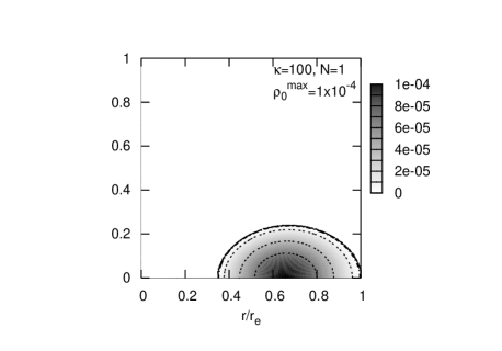
Figure 3: The distribution of $\rho_{0}$ of a spheroidal star (top) and a toroidal star (bottom) for $\kappa=100$, and $N=1$. For the spheroidal star, $\rho_{0}^{\rm{max}}=0.001$ and $r_{p}/r_{e}=0.7$ are used as input parameters, which are the same for the model shown in Fig. 1. The physical size $(r_{e})$ and the rotation frequency ($f_{rot}$) are 16.6 km and 597 Hz, respectively. For the toroidal star, $\rho_{0}^{\rm{max}}=0.0001$ and $r_{p}/r_{e}=-0.35$. The physical size is 49.6 km and the rotation frequency is 199 Hz.

As expected, our solutions show typical features of polytropic rotating stars. If $\kappa$ increases, the size of star increases and the rotation speed decreases. The density falls off more rapidly, the size becomes bigger, and the rotation speed becomes smaller as $N$ increases.

5.1.2 Relation between axis ratio and angular velocity

In Figures 4, we show equilibrium solution sequences of angular speed as a function of ellipticity which is defined as $\varepsilon=1-r_{p}/r_{e}$, for different choices of $\rho_{0}^{\rm{max}}$’s, represented by different line types, and three differnt values of polytropic indices ($N$), separated by different panels. The values of $\kappa$ are differnt for different choices of $N$: $N=1$ and $\kappa=100$ for the top, $N=1.5$ and $\kappa=10$ for the middle, and $N=3$ and $\kappa=0.1$ for the bottom panel. Each panel has three sequences which are three different values of $\rho_{0}^{\rm{max}}$: $10^{-2}$, $10^{-3}$, and $10^{-4}$. Note that the values of $R$ for the $\rho_{0}^{\rm{max}}=10^{-2}$, $10^{-3}$ and $10^{-4}$ are 2, 0.2, and 0.02 for $N=1$, and $R=1.16$, 0.25 and 0.054 for $N=1.5$ and $R=0.086$, 0.04 and 0.019 for $N=3$ respectively.

As shown in the figures, $\Omega_{C}$ increases with $\rho_{0}^{\rm{max}}$ and the sequences terminates at the critical rotation speed beyond which the mass shedding occurs. For the Newtonian case, due to the simple scaling property of $\Omega_{C}\propto\sqrt{\rho_{0}^{\rm{max}}}$, the critical rotation always occurs at the same $r_{p}/r_{e}$ (Hachisu, 1986a). However, our model shows somewhat different results. For the cases of $N=1$ and $N=1.5$, high density models are relativistic but low density models are not. The scaling relation of $\Omega_{C}\propto\sqrt{\rho_{0}^{{\rm max}}}$ does not hold if the models are relativistic. However, we found that the models with $N=3$ are all non-relativistic, and three different models with different $\Omega_{C}$ follows the Newtonian scaling relationship very well. The maximum value of ellipticity (or minimum values of axis ratio) are also nearly the same for different $\rho_{0}^{max}$.

Also shown in the inlets of each panel are the $\Omega_{C}/\Omega_{C,max}$ versus $\varepsilon/\varepsilon_{max}$ where the maximum values of $\Omega_{C}$ and $\varepsilon$ correspond to the critically rotating models. In such normalizations,the behavior of $\Omega_{C}$ with $\varepsilon$ is almost identical for models with different density if the polytropic index is fixed. For different $N$, however, the behaviour of $\Omega_{C}$ becomes somewhat different. Thus we conclude that the scaling relationship of $\Omega_{C}$ with $\varepsilon$ depends on the degree of relativity while the functional behaviour is mostly determined by the equation of state.

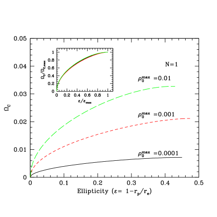
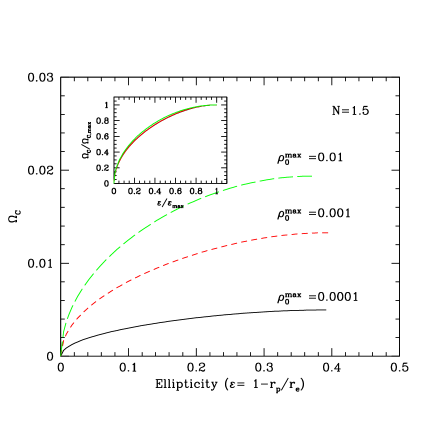
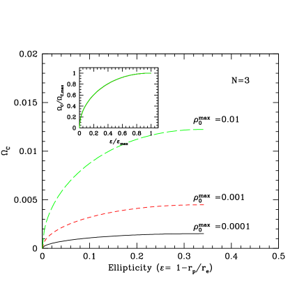
Figure 4: The rotation angular speed at the rotation axis ($\Omega_{C}$) versus the ellipticity for $N=1~{}(\Gamma=2)$, $N=1.5~{}(\Gamma=5/3)$, and $N=3~{}(\Gamma=4/3)$ from top to bottom panels. The three lines in each panel represent the results with $\rho_{0}^{\rm{max}}=0.01$, $0.001$ and $0.0001$ from the top. The corresponding values of $R$ defined in equation (16) from the top are: $R=2$, 0.2, and 0.02 for $N=1$, and 1.16, 0.25, and 0.054 in case of $N=1.5$, and 0.086, 0.040 and 0.0186, respectively. We also show the normalized angular speed versus normalized ellipticity in the inlet of each panel. These figures show that the functional behaviour of the angular speed at the rotational axis mostly depends on the equation of state.

5.1.3 Constant Rest Mass Sequences

Most of the neutron stars have their masses near the Chandrasekhar limit ($1.4M_{\odot}$). Even if they undergo dynamical changes, the baryon number of the star is conserved. Hence, the sequences in fixed rest mass can give an insight into the neutron stars’ dynamical properties. The rest mass of the star is obtained by

$$M_{0} = \int\rho_{0}u^{t}\sqrt{-g}d^{3}x$$ (20)

$$= 2\pi\int dr\int d\theta r^{2}\sin\theta\frac{\rho_{0}}{\sqrt{1-v^{2}}}\left(1+2\Phi\right)^{-\frac{3}{2}}.$$

In order to obtain the constant mass models, we adjusted the maximum density while keeping the equation of states unchanged.

Figure 5: Axis ratio ($r_{p}/r_{e}$) - maximum rest mass density ($\rho_{0}^{\rm{max}}$) relation in constant masses ($1.4M_{\odot}$ and $2M_{\odot}$) for spheroid (top panel) and toroid (bottom panel).

Figure 5 shows the relation between the axis ratio ($r_{p}/r_{e}$) and maximum rest mass density ($\rho_{0}^{\rm{max}}$). Since more elongated figures rotates faster and their sizes are larger, they do not need the large value of $\rho_{0}^{\rm{max}}$. Accordingly, $\rho_{0}^{\rm{max}}$ decreases as axis ratio decreases for spheroid and toroid. For the toroidal case, the density is much smaller than the spheroidal one and its size is very sensitively dependent on the value of $\rho_{0}^{\rm{max}}$.

Figure 6: Axis ratio ($r_{p}/r_{e}$) - rotational frequency relation in constant masses ($1.4M_{\odot}$ and $2M_{\odot}$) for spheroid (top panel) and toroid (bottom panel).

The relation between the rotation frequency at the axis versus ratio ($r_{p}/r_{e}$) relations is shown in Figure 6 for spheroidal (top panel) and toroidal cases (bottom panel). Of course more elongated shape and massive star rotates faster for spheroidal shape. Rotation frequency of toroid is much smaller than the one for spheroid since the specific angular momentum is larger for a given rotational frequency. For the $1.4M_{\odot}$ spheroidal star, rotational frequency is 539 Hz near the critical rotation and 724 Hz for the $2M_{\odot}$ one. For the toroidal stars, the critical frequencies become 215 and 280 Hz for 1.4 and 2.0 $M_{\odot}$, respectively.

Figure 7: Rotational frequency $\Omega$) - $T/|W|$ relation for the models with fixed total masses ($1.4M_{\odot}$ and $2M_{\odot}$) for spheroid (top panel) and toroid (bottom panel).

Figure 7 shows the relation between $\Omega_{C}$ and the ratio of the rotational kinetic energy to gravitational potential energy ($\beta\equiv T/|W|$). It is well known that a bar mode instability occurs if $\beta$ exceeds certain critical value $\beta_{d}$. For Newtonian case, the $\beta_{d}$ for the onset of the bar mode instability is 0.2738 (Chandrasekhar, 1969; Shapiro & Teukolsky, 1983). For the case of fully relativistic stars, the $\beta_{d}$ lies between 0.24 and 0.25 (Shibata, Baumgarte & Shipiro, 2001) which is slightly smaller than Newtonian one. The rotational kinetic energy ($T$) and gravitational potential energy ($W$) are defined as

$$T = \frac{1}{2}\int d^{3}x\Omega T^{t}_{\phi}\sqrt{-g}$$ (21)

$$= \frac{1}{2}\int d^{3}x\rho_{0}H\frac{v2}{1-v2}\sqrt{-g},$$

$$W=T+M_{p}-M_{\rm{active}},$$ (22)

where the proper mass $M_{p}$ and active mass $M_{\rm{active}}$ can be obtained by

$$M_{p}=\int d^{3}x\frac{\rho_{0}\left(1+\epsilon\right)}{\sqrt{1-v^{2}}}\sqrt{\gamma},$$ (23)

$$M_{\rm{active}}=\int d^{3}x\rho_{\rm{active}}\sqrt{-g}.$$ (24)

Like in Figure 6, upper panel and low panel of Figure 7 are for spherpidal and toroidal stars, respectively. We find that $T/|W|$ is much smaller than the critical values of bar mode instability for uniformly rotating spheroids with masses 1.4 and 2.0 $M_{\odot}$. On the other hand, all the sequences of toroidal models have $T/|W|$ greater than the instability criteria. Apparently, the toriodal configurations are all dynamically unstable.

5.2 Differentially Rotating Models

5.2.1 Solution of the Quasi-toroidal Objects

For differentially rotating stars, the angular frequency at the boundary becomes much smaller than the uniformly rotating stars in general since the inner parts rotate much faster than outer parts. Therefore, solutions could exist well below the critical rotational frequcncy for mass shedding of the uniformly rotating stars and the resulting shape of the star is quasi-toroidal. In figure 8, we show an example of quasi-toroidal distribution of $\rho_{0}$ for the same parameters with the uniformly rotating spheroidal star in Figure 3 (i.e., $\kappa=100$, $N=1$, and $\rho_{0}^{\rm max}$=0.001), except for $A^{2}$ which was taken to be 10. Also, the axis ratio was chosen to be $r_{p}/r_{e}=0.35$. The equatorial radius for this model is 17.4 km when the mass of the star is assumed to be 1.4 $M_{\odot}$. The resulting density distribution is a quasi-toroidal one in the sense that density does not vanish at the center. The maximum density, however occurs at finite radius so that the location of the maximum density is a ring, as already seen from Figure 2. The rotational frequency at the center is 5510 Hz, but it reduces to about 220 Hz at the surface.

The dependence of the rotation speed distribution on the parameter $A^{2}$ is shown in Figure 9. For $A^{2}=10$, the rotation speed at the equatorial boundary reduces to 10% of the one at the center. As expected, the rotation speed falls off more rapidly as $A$ decreases and becomes uniform as $A$ increases.

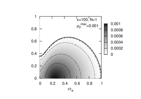
Figure 8: The distribution of $\rho_{0}$ for the quasi-toroidal example. The model parameters are the same as that of the spherdoidal example shown in Figure 3 (i.e., $\kappa=100$, $N=1$, and $\rho_{0}^{\rm{max}}=0.001$. The axis ratio of $r_{p}/r_{e}=0.35$, and $A^{2}=10$ are chosen for the rotational parameters. The resulting equatorial radius is 17.4 km, when the baryon mass is assumed to be 1.4 $M_{\odot}$ (see Figure 13). The rotation frequency at the center is $f_{C}=5510\rm{Hz}$ but it reduces down to 4 % of $f_{C}$ at the equatorial boundary.

Figure 9: The angular frequency distributions of the models with the same parameters as that one shown in Figure 8, but three different values of $A^{2}$=1, 10 and 100.

5.2.2 Constant Rest Mass Sequences

In this section, we describe the characteristics of the models with constant baryonic masses of 1.4 and 2 $M_{\odot}$ for differentially rotating objects with $A^{2}$=10 and 100. Unlike the uniform rotation, critical rotation for mass shedding does not occur in thses values of $A$.

Figure 10: Maximum rest mass density ($\rho_{0}^{\rm{max}}$) versus axis ratio ($r_{p}/r_{e}$) relation for models with two constant masses ($1.4M_{\odot}$ and $2M_{\odot}$) and two rotational parameters of $A^{2}=10$ (top panel) and $A^{2}=100$ (bottom panel).

Figure 10 shows that the relation between axis ratio ($r_{p}/r_{e}$) and maximum rest mass density ($\rho_{0}^{\rm{max}}$). Almost similar trend to uniformly rotating models is seen but $\rho_{0}^{\rm{max}}$ falls off more rapidly toward the smaller axis ratio. Also the maximum densities are generally larger than the toroidal figures of uniformly rotating models, but comparable to that of spheroidal models.

Figure 11 presents relationship between the axis ratio ($r_{p}/r_{e}$) and the rotational angular speed at the axis of rotation for the differentially rotating models shown in Figure 10. Note that the rotational frequency in units of Hz can be obtained by multiplying the rotational angular speed shown in this figure by 3.23 $\times 10^{4}$. Therefore, the rotational frequcncy at the axis of rotation could reach 6130 Hz and 4580 Hz for 1.4 and 2 $M_{\odot}$ models, respectively for the case of $A^{2}=10$. For the case of $A^{2}=100$, the rotational speed at the axis of rotation becomes 1520 and 1170 Hz for 1.4 and 2 $M_{\odot}$ models, respectively.

Figure 11: Rotation angular speed along rotation axis ($\Omega_{C}$) versus axis ratio ($r_{p}/r_{e}$) for the models with constant total masses ($1.4M_{\odot}$ and $2M_{\odot}$) and differential rotation parameter $A^{2}=10$ (top panel) and $A^{2}=100$ (bottom panel).

Figure 12: The relationship between $T/|W|$ and axis ratio for stars with $M_{0}=1.4M_{\odot}$ (solid) and $M_{0}=2M_{\odot}$ (dotted) for rotation parameters of $A^{2}=10$ (top panel) and $A^{2}=100$ (bottom panel).

Figure 12 shows $T/|W|$ as a function of the axis-ratio for the models shown in Figures 10 and 11. As we stated in the previous section, larger $A$ value makes the angular speed distribution nearly constant (i.e., uniform rotation). Therefore, rotational energy ($T$) tends to become larger for larger $A$. The most rapidly rotating models with $A^{2}=10$ have $T/|W|$=0.17 and 0.21 for the cases with baryon mass 1.4 and 2 $M_{\odot}$ while models with $A^{2}=100$ can have $T/|W|$=0.27 and 0.31 for $M=1.4$ and 2 $M_{\odot}$, respectively. Note, for differentially rotating stars, the onset of the dynamical instabilty depends on the strength of the differential rotation. For weak case, it turned out that $\beta_{d}\sim 0.27$ for Newtonian stars, just similar to the uniform rotation (see, for example, Liu & Lindholm (2001)). However, many stuides have found that it could be down to $\beta_{d}=0.2$ (Karino & Eriguchi, 2003), $\beta_{d}=0.14$ (Centrella et al., 2001; Tohline & Hachisu, 1990; Pickett, Durisen & Davis, 1996; Liu & Lindholm, 2001; Liu, 2002), and even down to 0.04 (Shibata, Karino, & Eriguchi, 2002, 2003). Recent full GR simulation has found $\beta_{d}$ = 0.254 for weak case (Baiotti et al., 2007).

6 Summary and Discussion

In order to find equilibrium solutions of rapidly rotating compact stars which have relativistic motions or relativistic equations of states, we have proposed an approximate method which is appropriate if the gravitational field is not very strong. Assuming the weak gravity, the spacetime and the hydrostatic equations are derived by only considering the Newtonian gravitational potential. However, in order to accommodate the relativistic effects, we have adopted the active mass density as a source for the gravitational potential. The active mass density takes into account all the forms of energy density. The numerical calculation has been carried out by following the Hachisu’s SCF method. We have obtained the equilibrium solutions for a wide range of parameters and topological shapes such as spheroid, toroid, and quasi-toroid. Only the polytropic equation of state is considered for simplicity. The inclusion of special relativistic effects could significantly improve the accuracy of the solutions if the rotational speed is substantial compared to the purely Newtonian hydrodynamical approach. We have shown that the solutions can be further improved by taking into account the the contribution from the active mass density for the computation of the gravitational field. Even for a mildly relativistic case ($R\sim 0.1$), we found that the active mass plays important role.

We have concentrated only on the equilibrium models in this paper. The studies on the stability of the relativistic stars and their physical sequences should be followed by integrating dynamical equations. In the subsequent works, we will provide the full set of dynamical equations under the same assumptions (i.e., Newtonian gravity with active mass and special relativistic hydrodynamics) and carry out the dynamical evolution studies of rapidly rotating compact stars.

This work was supported by the Korean Research Foundation Grant No. 2006-341-C00018. JK acknowledges the support BK21 program to SNU.

References

- Baiotti et al. (2007) Baiotti, L., Pietri, R. De, Manca, G. M., Rezzolla, L., 2007, Phys. Rev. D, 75, 044023
- Baumgarte et al. (1998) Baumgarte, T. W., Cook, G. B., Scheel, M. A., Shapiro, S. L., & Teukolsky, S. A., 1998, PRD, 57, 7299
- Centrella et al. (2001) Centrella, J. M., New, K. C. B., Lowe, L, & Brown, J. D., 2001, ApJ, 550, L193
- Chandrasekhar (1969) Chandrasekhar, S., 1981, Ellipsoidal Figures of Equilibrium, Yale Univ. Press, New Haven
- Cook et al. (1992) Cook, G. B., Shapiro, S. L., & Teukolsky, S. A. 1992, ApJ, 398, 203
- Cook et al. (1994a) —–. 1994, ApJ, 422, 227
- Cook et al. (1994b) —–. 1994, ApJ, 424, 823
- Dyson (1983a) Dyson, F. W., 1893, Roy. Soc. of London Philosophical Trans. Ser. A, 184, 43
- Dyson (1983b) —–. 1893, Roy. Soc. of London Philosophical Trans. Ser. A, 184, 1041
- Eriguchi & Sugimoto (1981) Eriguchi, Y., & Sugimoto, D. 1981, Progress of Theoretical Physics, 65, 1870
- Fischer et al. (2005) Fischer, T., Horatschek, S., & Ansorg, M. 2005, MNRAS, 364, 943
- Font (2008) Font, J. A. 2008, Living Reviews in Relativity, 11, 7
- Hachisu (1986a) Hachisu, I. 1986, ApJS, 61, 479
- Hachisu (1986b) —–. 1986, ApJS, 62, 461
- James (1964) James, R. A. 1964, ApJ, 140, 552
- Kaaret et al. (2007) Kaaret, P., et al. 2007, ApJ, 657, L97
- Karino & Eriguchi (2003) Karino, S. & Eriguchi, Y., 2003, ApJ, 592, 1119
- Kiuchi & Kotake (2008) Kiuchi, K., & Kotake, K. 2008, MNRAS, 385, 1327
- Komatsu et al. (1989a) Komatsu, H., Eriguchi, Y., & Hachisu, I. 1989, MNRAS, 237, 355
- Komatsu et al. (1989b) Komatsu, H., Eriguchi, Y., & Hachisu, I. 1989, MNRAS, 239, 153
- Labranche et al. (2007) Labranche, H., Petroff, D., & Ansorg, M. 2007, Gen. Rel. Grav., 39, 129
- Liu (2002) Liu, Y. T. 2002, Phys. Rev. D, 65, 124003
- Liu & Lindholm (2001) Liu, Y. T. & Lindholm, L., 2001, MNRAS, 342, 1063
- Ostriker & Mark (1968) Ostriker, J. P., & Mark, J. W.-K. 1968, ApJ, 151, 1075
- Ou & Tohline (2006) Ou, S., & Tohline, J. E. 2006, ApJ, 651, 1068
- Petroff & Horatschek (2008) Petroff, D., & Horatschek, S. 2008, MNRAS, 389, 156
- Pickett, Durisen & Davis (1996) Pickett, B. K., Durisen, R. H. & Davis, G. A., 1996, ApJ, 458,714
- Shapiro & Teukolsky (1983) Shapiro, S. L. & Teukolsky, S. A., 1983, Black Holes, White Dwarfs, and Neutron Stars, John Wiley and Sons, New York
- Shibata, Baumgarte & Shipiro (2001) Shapiro, S. L., Baumgarte, T. W., 2002, ApJ, 542, 453
- Shibata, Karino, & Eriguchi (2002) Shibata, M., Karino, S. & Eriuguchi, Y., 2002, MNRAS, 334, L27
- Shibata, Karino, & Eriguchi (2003) Shibata, M., Karino, S. & Eriuguchi, Y., 2002, MNRAS, 343, 619
- Stergioulas & Friedman (1995) Stergioulas, N., & Friedman, J. L. 1995, ApJ, 444, 306
- Stoeckly (1965) Stoeckly, R. 1965, ApJ, 142, 208
- Tohline & Hachisu (1990) Tohline, J. E., & Hachisu, I. 1990, ApJ, 361, 394
- Tolman (1934) Tolman, R. C. 1934, Relativity, Thermodynamics, and Cosmology, Oxford: Clarendon Press, 1934,
- Varga (1962) Varga, R. S. 1962, Matrix Iterative Analysis, Prentice-Hall, Eaglewood Cliffs, NJ.
- Wong (1974) Wong, C.-Y. 1974, ApJ, 190, 675