Shrinkage regression for multivariate inference with missing data, and an application to portfolio balancing

Abstract

Portfolio balancing requires estimates of covariance between asset returns. Returns data have histories which greatly vary in length, since assets begin public trading at different times. This can lead to a huge amount of missing data—too much for the conventional imputation-based approach. Fortunately, a well-known factorization of the MVN likelihood under the prevailing historical missingness pattern leads to a simple algorithm of OLS regressions that is much more reliable. When there are more assets than returns, however, OLS becomes unstable. Gramacy et al., (2008) showed how classical shrinkage regression may be used instead, thus extending the state of the art to much bigger asset collections, with further accuracy and interpretation advantages. In this paper, we detail a fully Bayesian hierarchical formulation that extends the framework further by allowing for heavy-tailed errors, relaxing the historical missingness assumption, and accounting for estimation risk. We illustrate how this approach compares favorably to the classical one using synthetic data and an investment exercise with real returns. An accompanying R package is on CRAN.

Key words: multivariate, monotone missing data, data augmentation, ridge regression, double-exponential, heavy tails, factor model, portfolio balancing

1 Introduction

Mean–variance portfolio allocation (e.g., Markowitz,, 1959) requires the accurate and tractable estimation of the mean return, and the covariance between the returns, of a large number of assets. Assets become publicly tradeable at different times, so their return histories can greatly vary in length. Aside from a few “gaps”, the histories of assets which are publicly tradeable at purchase time will exhibit a monotone missingness pattern. For example, Figure 1 shows the monthly return availability for 1,200-odd stocks on NYSE & AMEX over 29 years, some with as little as 1 years worth of data.

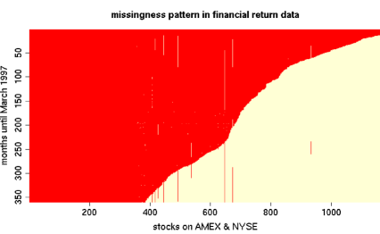
Figure 1: Missingness pattern in stock returns on the NYSE & AMEX. The assets (columns) are put into increasing order of the number of missing entries.

The assets along the columns have been sorted by the number of missing entries. Besides some “gaps” the boundary between the dark and light regions is monotone.

Generally speaking, inference in the presence of missing data is notoriously difficult, usually requiring hill-climbing iterative techniques like expectation maximization (Little and Rubin,, 2002; Schafer,, 1997)) which rapidly lose stability as the level of missingness increases. The Bayesian alternative of data augmentation is similarly unsatisfactory. Software packages implementing such algorithms come with prominently displayed warnings of failure when the missingness level is above 15% (see Gramacy et al.,, 2008).

The nice thing about a monotone missingness pattern is that the likelihood has a convenient factorization which makes inference tractable without imputation. Under a multivariate normal (MVN) assumption, a simple algorithm (Andersen,, 1957; Stambaugh,, 1997) of ordinary least squares (OLS) regressions, one for each asset, yields a maximum likelihood estimator (MLE). Unfortunately, there must be fewer stocks than the length of the shortest return history, so that the design matrices of the OLS regressions are of full rank. In particular, you cannot have more stocks than historical returns. Gramacy et al., (2008) showed that by replacing the OLS with “parsimonious regressions”, e.g., principal components (PCR), ridge, lasso, etc., the above algorithm can be applied when there are more assets than historical returns. This extended the reach of Stambaugh’s (1997) methods from dozens to thousands of assets, accommodating an essentially arbitrary level of historical missingness.

In this paper we shall further extend the above parsimonious methodology in several directions by taking a fully Bayesian approach. Section 2 recalls the monotone decomposition and (MLE/Bayesian) inference algorithm. Section 3 reviews approaches to Bayesian shrinkage regression that are particularly convenient in this context, and which allow model averaging and heavy-tailed errors as minor embellishments. Section 4 details how the benefits of the Bayesian shrinkage posteriors filter through to inference about the mean vector and covariance matrix. It features extensions for data augmentation to deal with “gaps”, and allows estimation risk to influence the balanced portfolios—both of which were unavailable previously. In Section 5 we apply our methods in a Monte Carlo investment exercise and show how they compare favorably to the classical alternatives on real financial returns data. The paper concludes with a brief discussion in Section 6.

The methods that are core to this paper are implemented in a fully documented R (R Development Core Team,, 2007) package called monomvn (Gramacy,, 2009), which is available for download on the Comprehensive R Archive Network (CRAN).

2 Multivariate normal monotone missing data

We assume that the missingness mechanism is missing completely at random (MCAR). In the case of historical asset returns this may be a tenuous assumption, but it is convenient and common (e.g., Stambaugh,, 1997). We work with a $n\times m$ data matrix $\mathbf{Y}$ that collects the historical returns of the assets. Denote $y_{i,j}=\mbox{\tt NA}$ if the $i^{\mbox{\tiny th}}$ sample (historical return) of the $j^{\mbox{\tiny th}}$ covariate (asset) is missing; otherwise $y_{i,j}\in\mathbb{R}$. Formally speaking, the missingness pattern in $\mathbf{Y}$ is said to be monotone [e.g., (Schafer,, 1997, Section 6.5.1) or (Little and Rubin,, 2002, Section 7.4)] if its columns can be re-arranged so that $y_{i,j}\neq\mbox{\tt NA}$ whenever $y_{i,j+1}\neq\mbox{\tt NA}$.

We assume throughout that they are indeed arranged in this way, so that when we define $n_{j}=\sum_{i=1}^{n}\mathbb{I}_{\{y_{i,j}\neq\,\mbox{\tt\footnotesize NA}\}}$ as the number of observed entries in column $j$, for $j=1,\dots,m$, we have that $n\equiv n_{1}$ and $n_{j}\geq n_{j+1}$. Furthermore, the rows may be arranged according to the same property ($y_{i,j}\neq\mbox{\tt NA}$ whenever $y_{i+1,j}\neq\mbox{\tt NA}$) without loss of generality, so that when we define $\mathbf{y}_{j}\equiv y_{1:n_{j},j}$ we are collecting the entirety of the observed entries in the $j^{\mbox{\tiny th}}$ column.

Figure 2: Diagram of a monotone missingness pattern with $m=6$ covariates, and $n$ completely observed samples in $\mathbf{y}_{1}=y_{:,1}$. The design matrix $\mathbf{Y}_{5}$ (without an intercept term) and the response vector $\mathbf{y}_{5}$ for the fifth regression involved in maximizing the likelihood of MVN data under a monotone missingness pattern is also shown. Time $(t)$ runs counter to the index $i$ so that the most recent historical return is at time $t=n$, indexed by $i=1$.

The pattern that results is illustrated pictorially in Figure 2. For now we will assume that there are no “gaps”. It is also helpful to define $\mathbf{Y}_{j}\equiv\mathbf{Y}_{0:(j-1)}^{(n_{j})}$ as the $n_{j}\times j$ design matrix

$$\mathbf{Y}_{j}\equiv\mathbf{Y}_{0:(j-1)}^{(n_{j})}=\begin{pmatrix}1&y_{1,1}&\cdots&y_{1,(j-1)}\\ 1&y_{2,1}&\cdots&y_{2,(j-1)}\\ \vdots&\vdots&\ddots&\vdots\\ 1&y_{n_{j},1}&\cdots&y_{n_{j},(j-1)}\end{pmatrix}$$

containing an intercept, and the first $n_{j}$ rows of the first $j-1$ columns of $\mathbf{Y}$; see Figure 2.

Under the monotone pattern the likelihood $f(\mathbf{Y}|\mbox{\boldmath$\theta$})$ emits a convenient factorization in terms of an auxiliary parameterization $\mbox{\boldmath$\phi$}=\Phi(\mbox{\boldmath$\theta$})$. If the rows of $\mathbf{Y}$ are i.i.d. MVN, this factorization leads to an iterative algorithm for inferring the MLE $\hat{\mbox{\boldmath$\theta$}}=(\hat{\mbox{\boldmath$\mu$}},\hat{\mbox{\boldmath$\Sigma$}})$. These assumptions may not be appropriate for financial returns but they are common to keep inference tractable (e.g., Stambaugh,, 1997; Chan et al.,, 1999; Jagannathan and Ma,, 2003).

The algorithm, due originally to Andersen, (1957), begins by calculating $\hat{\mu}_{1}$ and $\hat{\Sigma}_{1,1}\equiv\hat{\sigma}_{1}^{2}$ in the usual way: $\hat{\mu}_{1}=n_{1}^{-1}\sum_{i=1}^{n_{1}}y_{i,1}$ and $\hat{\sigma}_{1}^{2}=n_{1}^{-1}\sum_{i=1}^{n_{1}}(y_{i,1}-\hat{\mu}_{1})^{2}$. Then, for $j=2,\dots,m$ the MLEs of $\mbox{\boldmath$\theta$}_{j}=(\mu_{j},\mbox{\boldmath$\Sigma$}_{1:j,j})$, $j=2,\dots,m$, can then be obtained via a regression on the complete data in columns $1,\dots,j-1$, i.e., using the model $\mathbf{y}_{j}=\mathbf{Y}_{j}\mbox{\boldmath$\beta$}_{j}+\mbox{\boldmath$\epsilon$}_{j}$, where $\{\epsilon_{i,j}\}_{i=1}^{n_{j}}\stackrel{{\scriptstyle\mathrm{iid}}}{{\sim}}\mathcal{N}(0,\sigma_{j}^{2})$. Here $\mbox{\boldmath$\beta$}_{j}^{\top}=(\beta_{0,j},\beta_{1,j},\dots,\beta_{(j-1),j})$, and $\sigma_{j}^{2}$ are the auxiliary parameters $\mbox{\boldmath$\phi$}_{j}$. When $\mathrm{rank}(\mathbf{Y}_{j})=j$, and particularly when $n_{j}>j$, MLEs $\hat{\mbox{\boldmath$\phi$}}_{j}$ may be obtained in the usual way: $\hat{\mbox{\boldmath$\beta$}}_{j}=(\mathbf{Y}_{j}^{\top}\mathbf{Y}_{j})^{-1}\mathbf{Y}_{j}^{\top}\mathbf{y}_{j}$ and $\hat{\sigma}^{2}_{j}=\frac{1}{n_{j}}||\mathbf{y}_{j}-\mathbf{Y}_{j}\hat{\mbox{\boldmath$\beta$}}_{j}||^{2}=\frac{1}{n_{j}}\sum_{i=1}^{n_{j}}(y_{i,j}-(\mathbf{y}_{i}^{\top})_{1:n_{j}}\,\hat{\mbox{\boldmath$\beta$}}_{j})^{2}$. The components of $\hat{\mbox{\boldmath$\theta$}}_{j}$ given $\hat{\mbox{\boldmath$\theta$}}_{1:(j-1)}=(\hat{\mbox{\boldmath$\mu$}}_{1:(j-1)}^{\top},\hat{\mbox{\boldmath$\Sigma$}}_{1:(j-1),1:(j-1)})$ and $\hat{\mbox{\boldmath$\phi$}}_{j}$ are then

$$\hat{\mu}_{j} =\hat{\beta}_{0,j}+\hat{\mbox{\boldmath$\beta$}}_{1:(j-1),j}^{\top}\hat{\mbox{\boldmath$\mu$}}_{1:(j-1)} \hat{\mbox{\boldmath$\Sigma$}}_{1:j,j} =\begin{pmatrix}\hat{\mbox{\boldmath$\beta$}}_{1:(j-1),j}^{\top}\hat{\mbox{\boldmath$\Sigma$}}_{1:(j-1),1:(j-1)}\\ \hat{\sigma}^{2}_{j}+\hat{\mbox{\boldmath$\beta$}}_{1:(j-1),j}^{\top}\hat{\mbox{\boldmath$\Sigma$}}_{1:(j-1),1:(j-1)}\hat{\mbox{\boldmath$\beta$}}_{1:(j-1),j},\end{pmatrix}.$$ and (1)

The $\hat{\mbox{\boldmath$\Sigma$}}$ thereby obtained will be positive-definite, as long as $n_{j}>j$ for all $j=1,\dots,m$ so that $\mathbf{Y}_{j}$ is of full rank, and $\mathbf{Y}_{j}^{\top}\mathbf{Y}_{j}$ invertible.

2.1 Bayesian inference

The Bayesian approach follows naturally from priors on the auxiliary parameters $\mbox{\boldmath$\beta$}_{j}$ and $\sigma_{j}^{2}$, for $j=1,\dots,m$. Samples from the implied posterior of $\mu_{j}$ and $\mbox{\boldmath$\Sigma$}_{1:j,j}$ are then obtained via $\Phi^{-1}$ in Eq. (1). It may be more desirable to choose priors directly in the natural parameter space $\mbox{\boldmath$\theta$}=(\mbox{\boldmath$\mu$},\mbox{\boldmath$\Sigma$})$, but it can be difficult to analytically derive the implied priors for $\mbox{\boldmath$\beta$}_{j}$ and $\sigma_{j}^{2}$. However, a popular non-informative prior used for MVN data, $p(\mbox{\boldmath$\mu$},\mbox{\boldmath$\Sigma$})\propto|\mbox{\boldmath$\Sigma$}|^{-\left(\frac{m+1}{2}\right)}$, can be shown (Schafer,, 1997, Section 6.5.3) to imply the (independent) prior(s) $p(\mbox{\boldmath$\beta$}_{j},\sigma_{j}^{2})\propto(\sigma_{j}^{2})^{-\left(\frac{m+1}{2}-m+j\right)}$, giving the posterior conditionals:

$$\mbox{\boldmath$\beta$}_{j}|\sigma^{2}_{j},\mbox{\boldmath$y$}_{j},\mbox{\boldmath$Y$}_{j} \sim\mathcal{N}_{j}(\hat{\mbox{\boldmath$\beta$}}_{j},\sigma^{2}_{j}(\mbox{\boldmath$Y$}_{j}^{\top}\mbox{\boldmath$Y$}_{j})^{-1})$$

$$\sigma^{2}_{j}|\mathbf{y}_{j},\mathbf{Y}_{j} \sim\mathrm{IG}((n_{j}-m+j-1)/2,(||\mathbf{y}_{j}-\mathbf{Y}_{j}\hat{\mbox{\boldmath$\beta$}}_{j}||^{2})/2).$$

Stambaugh, (1997) showed that, under this non-informative prior, it is possible to derive the moments of the Bayesian posterior predictive distribution in terms of the MLEs $(\hat{\mbox{\boldmath$\mu$}},\hat{\mbox{\boldmath$\Sigma$}})$ in closed form. When these are used in the mean–variance framework to construct portfolios, they are said to take estimation risk (Klein and Bawa,, 1976; Brown,, 1979) into account. However, these calculations similarly break down when $n_{j}\leq j$.

Inverted Wishart priors for $\Sigma$ are amenable to tractable posterior inference under the MVN with monotone missingness (Liu,, 1993). One example is a ridge prior (Schafer,, 1997, Section 5.2.3), which is helpful when $m>n$ and is closely related to ridge regression [see Section 3] as used by Gramacy et al., (2008) in $\phi$-space to good effect. This motivates a more pragmatic approach to prior selection: a deliberate search for appropriate shrinkage priors for the “big $p$ small $n$” regression problem in $\phi$-space, where the low rank $\mathbf{Y}_{j}$ problem is manifest. Then, $\Phi^{-1}$ completes the description implicitly in $\theta$-space.

3 Bayesian shrinkage regression

Here we focus on appropriate regression models for the “big $p$ small $n$” problem that employ shrinkage. The customary formulation is

$$\mathbf{y} =\beta_{0}\mathbf{1}_{n}+\mathbf{X}\mbox{\boldmath$\beta$}+\mbox{\boldmath$\epsilon$}, \mathbf{\epsilon} \sim\mathcal{N}_{n}(\mathbf{0},\sigma^{2}\mathbf{I}_{n}).$$ where (2)

One typically assumes a standardized $n\times p$ design matrix $\mathbf{X}$ where the columns are individually adjusted to have zero-mean and unit L2-norm. This causes $\beta_{0}$ and $\beta$ to be independent a posteriori and recognizes that regularized posterior summaries for $\beta$ are not equivariant under a re-scaling of $\mathbf{X}$. Any such pre-processing must be undone before evaluating $\mbox{\boldmath$\theta$}=\Phi^{-1}(\mbox{\boldmath$\phi$})$ at samples of $\mbox{\boldmath$\phi$}=(\beta_{0},\mbox{\boldmath$\beta$},\sigma^{2})$.

Ridge regression and the lasso (e.g., Hastie et al.,, 2001, Section 3.4.3) are classical approaches to shrinkage regression that penalize large coefficients:

$$\hat{\mbox{\boldmath$\beta$}}^{(q)}=\operatorname*{argmin}_{\mbox{\boldmath$\beta$}}\left\{(\tilde{\mathbf{y}}-\mathbf{X}\mbox{\boldmath$\beta$})^{\top}(\tilde{\mathbf{y}}-\mathbf{X}\mbox{\boldmath$\beta$})+\lambda\sum_{j=1}^{p}|\beta_{j}|^{q}\right\}$$ (3)

for some $\lambda\geq 0$, where the intercept is excluded from penalization via $\tilde{\mathbf{y}}=\mathbf{y}-\bar{y}\mathbf{1}_{n}$. Choosing $q=2$ yields ridge regression (Hoerl and Kennard,, 1970) where $\hat{\mbox{\boldmath$\beta$}}^{(2)}=(\mathbf{X}^{\top}\mathbf{X}+\lambda\mathbf{I})^{-1}\mathbf{X}^{\top}\mathbf{y}$. The lasso (Tibshirani,, 1996) corresponds to $q=1$. There is no closed form solution for $\hat{\mbox{\boldmath$\beta$}}^{(1)}$, but the entire path of solutions for all $\lambda$ can be obtained iteratively via the LARS algorithm (Efron et al.,, 2004). Both estimators may be interpreted as the posterior mode under a particular prior. For ridge regression the prior is $\mbox{\boldmath$\beta$}^{(2)}|\sigma^{2}\sim\mathcal{N}_{p}(\mathbf{0},\sigma^{2}\lambda\mathbf{I}_{p})$; for the lasso it is i.i.d. Laplace (i.e., double-exponential) $\pi(\mbox{\boldmath$\beta$}^{(1)}|\sigma^{2})=\prod_{j=1}^{p}\frac{\lambda}{2\sqrt{\sigma^{2}}}e^{-\lambda|\beta^{(1)}_{j}|/\sqrt{\sigma^{2}}}.$

Large values of the penalty parameter $\lambda$ cause the coefficients of $\hat{\mbox{\boldmath$\beta$}}^{(q)}$ to be shrunk towards zero. The lasso estimator $\hat{\mbox{\boldmath$\beta$}}^{(1)}$ may have many coefficients shrunk to exactly zero, which is convenient for variable selection. Often, $\lambda$ is chosen via cross validation (CV). As a $\phi$-space regression for obtaining monotone MVN estimators. Gramacy et al., (2008) chose $\lambda$ by applying the “one-standard-error” rule (Hastie et al.,, 2001, Section 7.10) with CV.

3.1 Hierarchical models for Bayesian shrinkage regression

For a fully Bayesian lasso we use the latent variable formulation of Park and Casella, (2008) and Carlin and Polson, (1991) by representing the Laplace as a scale mixture of normals:

$$\mathbf{y}|\beta_{0},\mathbf{X},\mbox{\boldmath$\beta$},\sigma^{2} \sim\mathcal{N}_{n}(\beta_{0}\mathbf{1}_{n}+\mathbf{X}\mbox{\boldmath$\beta$},\sigma^{2}\mathbf{I}_{n}) \mathbf{D}_{\tau} =\mathrm{diag}(\tau_{1}^{2},\dots,\tau_{p}^{2})$$ (4)

$$\mbox{\boldmath$\beta$}|\sigma^{2},\tau_{1}^{2},\dots,\tau_{p}^{2} \sim\mathcal{N}_{p}(\mathbf{0},\sigma^{2}\mathbf{D}_{\tau}),\;\;\beta_{0}\propto 1 \sigma^{2} \sim\mathrm{IG}(a_{\sigma}/2,b_{\sigma}/2)$$

$$\tau_{j}^{2}|\lambda \stackrel{{\scriptstyle\mathrm{iid}}}{{\sim}}\mathrm{Exp}(\lambda^{2}/2) \lambda^{2} \sim G(a_{\lambda},b_{\lambda}).$$

IG and G are the rate- and scale-parameterized inverse-gamma and gamma distributions, respectively. The default prior $\pi(\sigma^{2})\propto\sigma^{-2}$ is obtained with $a_{\sigma}=b_{\sigma}=0$, and ridge regression is the special case where $\tau^{2}\equiv\tau_{1}^{2}=\cdots=\tau_{p}^{2}$, using $\tau^{2}\sim\mathrm{IG}(a_{\tau}/2,b_{\tau}/2)$ (i.e., dropping $\lambda^{2}$), possibly with $a_{\tau}=b_{\tau}=0$. Fixing $\tau^{2}=\infty$ yields the standard family of (improper) priors for linear regression.

Choosing the prior parameterization for $\lambda^{2}$ can be difficult. Park and Casella, (2008) note that choosing $a_{\lambda}=b_{\lambda}=0$ leads to an improper posterior, and suggest some automatic alternatives. Another option is to further expand the hierarchy using a so-called normal-gamma (NG) prior for $\beta$ (e.g., Griffin and Brown,, 2010) by specifying

$$\lambda^{2}|\gamma \sim G(a_{\lambda},b_{\lambda}/\gamma),\;\;\;\;\;\mbox{where}\;\;\;\;\;\gamma\sim\mathrm{Exp}(1)$$ (5)

$$\mbox{and}\;\;\;\;\;\tau_{j}^{2}|\lambda^{2},\gamma \stackrel{{\scriptstyle\mathrm{iid}}}{{\sim}}G(\gamma,\lambda^{2}/2).$$

Griffin and Brown, (2010) suggest $a_{\lambda}=2$, and $b_{\lambda}=M/2$, where $M$ is chosen via empirical Bayes considerations. Observe that fixing $\gamma=1$ encodes the specific Laplace prior case. So the NG prior is more adaptive than the lasso. This may come in handy when $p\gg n$, i.e., when our prior plays a more important role, or when the posterior drives many $\beta_{j}$’s to zero.

The availability of full conditionals for all of the parameters makes for efficient Gibbs sampling (GS). For the baseline Bayesian lasso model (Park and Casella,, 2008) these are:

$$\beta_{0}|\sigma^{2},\mathbf{y} \sim\mathcal{N}(\bar{y},\sigma^{2}/n)$$

$$\mbox{\boldmath$\beta$}|\sigma^{2},\{\tau_{j}^{2}\}_{j=1}^{p},\mathbf{y} \sim\mathcal{N}_{p}(\tilde{\mbox{\boldmath$\beta$}},\sigma^{2}\mathbf{A}^{-1}), \mathbf{A} =\mathbf{X}^{\top}\mathbf{X}+\mathbf{D}_{\tau}^{-1},\;\;\tilde{\mbox{\boldmath$\beta$}}=\mathbf{A}^{-1}\mathbf{X}^{\top}\tilde{\mathbf{y}}$$

$$\sigma^{2}|\mbox{\boldmath$\beta$},\{\tau_{j}^{2}\}_{j=1}^{p},\mathbf{y} \sim\mathrm{IG}((a_{\sigma}+n-1+p)/2,(b_{\sigma}+\psi_{\beta})/2), \psi_{\beta} =||\tilde{\mathbf{y}}-\mathbf{X}\mbox{\boldmath$\beta$}||^{2}+\mbox{\boldmath$\beta$}^{\top}\mathbf{D}_{\tau}^{-1}\mbox{\boldmath$\beta$}$$

$$\tau_{j}^{-2}|\beta_{j},\sigma^{2},\lambda \stackrel{{\scriptstyle\mathrm{iid}}}{{\sim}}\mbox{Inv-Gauss}(\sqrt{\lambda^{2}\sigma^{2}/\beta_{j}^{2}},\lambda^{2})$$ (6)

$$\lambda^{2}|\tau_{1}^{2},\dots,\tau_{p}^{2} \sim\mbox{G}(a_{\lambda}+p\gamma,b_{\lambda}/\gamma+\textstyle\sum_{j=1}^{p}\tau_{j}^{2}/2). [\mbox{assuming }\gamma=1]$$

Using a marginal posterior conditional for $\sigma^{2}$ instead can help reduce autocorrelation in the Markov chain. Integrating over the posterior conditional for $\beta$ gives $\sigma^{2}|\tau_{1}^{2},\dots,\tau_{p}^{2},\mathbf{y}\sim\mathrm{IG}((a_{\sigma}+n-1)/2,(b_{\sigma}+\psi_{\tilde{\beta}})/2),$ where $\psi_{\tilde{\beta}}=||\tilde{\mathbf{y}}-\mathbf{X}\tilde{\mbox{\boldmath$\beta$}}||^{2}+\tilde{\mbox{\boldmath$\beta$}}^{\top}\mathbf{D}_{\tau}^{-1}\tilde{\mbox{\boldmath$\beta$}}=\tilde{\mathbf{y}}^{\top}\tilde{\mathbf{y}}-\tilde{\mbox{\boldmath$\beta$}}^{\top}\mathbf{A}\tilde{\mbox{\boldmath$\beta$}}$.

Under the ridge regression model the posterior conditionals are the same (6) except that we ignore $\lambda^{2}$ and take $\tau^{2}\sim\mathrm{IG}((a_{\tau}+p)/2,(b_{\tau}+\sigma^{-2}\mbox{\boldmath$\beta$}^{\top}\mbox{\boldmath$\beta$})/2)$. Upon fixing $\tau^{2}=\infty$ we must use $\mathbf{A}=\mathbf{X}^{\top}\mathbf{X}$, subtract $p/2$ to the rate parameter to the IG conditional(s) for $\sigma^{2}$, and ensure a proper posterior with $a_{\sigma}>p-n-1$. This may pose a non-trivial restriction on the prior when $p\geq n$. Under the NG prior $\gamma$ may vary, leading to the conditionals

$$\tau_{j}^{2}|\beta_{j},\sigma^{2},\lambda^{2},\gamma \stackrel{{\scriptstyle\mathrm{iid}}}{{\sim}}\mathrm{GIG}(\gamma-1/2,\beta_{j}^{2}/\sigma^{2},\lambda^{2})$$ (7)

$$\gamma|\{\tau_{j}^{2}\}_{j=1}^{p},\lambda^{2} \propto\left(\frac{\lambda^{2}}{2}\right)^{p\gamma}\frac{\pi(\gamma)}{(\Gamma(\gamma))^{p}}\left(\prod_{i=1}^{p}{\tau_{j}^{2}}\right)^{\gamma},$$

where $\mathrm{GIG}(\lambda,\chi,\psi)$ is the generalized inverse Gaussian distribution. Griffin and Brown, (2010) suggest a random walk Metropolis update for the $\gamma$ using proposals $\gamma^{\prime}=\exp\{\sigma_{\gamma}z\}$, for $z\sim\mathcal{N}(0,1)$. These proposals are accepted with probability

$$\min\left\{1,\frac{\pi(\gamma^{\prime})}{\pi(\gamma)}\left(\frac{\Gamma(\gamma)}{\Gamma(\gamma^{\prime})}\right)^{p}\left(\left(\frac{2}{\lambda^{2}}\right)^{-p}\prod_{i=1}^{p}\tau_{j}^{2}\right)^{\gamma^{\prime}-\gamma}\right\},$$ (8)

where $\pi(\gamma)=\gamma^{-2}\exp(-\gamma-\frac{M}{2\gamma}\lambda^{2})$ and $\sigma_{\gamma}$ is chosen to give an acceptance rate of 20-30%.

An alternative hierarchical modeling framework for the Bayesian lasso is provided by Hans, (2008). While it does not require $p$ latent $\tau^{2}_{j}$ variables, the resulting GS procedure is not fully blocked, and rejection sampling is required for $\sigma^{2}$. “Orthogonalizing” the sampler helps mitigate slow mixing of the un-blocked conditionals. However, we prefer the simpler approach of Park and Casella, (2008) as it is more readily adaptable to the $p\gg n$ case, to model selection, and our extensions to the heavy-tailed errors.

Whereas the classical lasso has the property that the estimate $\hat{\mbox{\boldmath$\beta$}}^{(1)}$ may have components which are zero—in fact, it would never have more than $\min\{p,n-1\}$ nonzero components— samples of $\beta$ from the posterior would never have zeros. So the Bayesian lasso is less useful for variable selection. We also note that when $p\geq n$—and without the ability to explicitly restrict $\beta$ to having at most $\min\{p,n-1\}$ nonzero components—a proper prior must be used for $\sigma^{2}$ or the posterior will be improper. An empirical Bayes remedy that works well in this case is to take a small $a_{\sigma}$, say $a_{\sigma}=3/2$, and then set $b_{\sigma}$ so that the $(1-\alpha)$ part of the IG($a_{\sigma},b_{\sigma})$ distribution lies at the point $\tilde{\mathbf{y}}^{\top}\tilde{\mathbf{y}}$ (i.e., the MLE under the intercept model) via the incomplete gamma inverse function. Another remedy is Bayesian model averaging.

3.2 Bayesian model selection and averaging

Although the MAP lasso fit may indeed set some of the coordinates of $\hat{\mbox{\boldmath$\beta$}}^{(1)}$ to zero, this is more of a side effect of the solution space of the quadratic program (3) than the result of a deliberate prior modeling choice (Hans,, 2008). Bayesians rarely base inference on the MAP; it is more natural to select variables by inspecting the posterior model probabilities.

There are several standard ways of performing Bayesian variable selection in regression models that are amenable to GS. They essentially fall into two camps. Loosely, the first camp (e.g., Geweke,, 1996; George and McCulloch,, 1993) uses a product-space wherein the prior for each $\beta_{j}$ is augmented to include a point-mass at zero. Inference proceeds by GS on each of the conditionals $\beta_{j}|\mbox{\boldmath$\beta$}_{-j},\mathbf{y},\dots$, $j=1,\dots,p$, which may flop between zero and nonzero values. Hans, (2008) augmented this product space approach to variable selection under the Laplace prior by further conditioning on $\lambda$.

The second camp (e.g., Troughton and Godsill,, 1997) is transdimensional in that the $\beta$-vector may vary in length while model space is traversed via Reversible Jump (RJ) MCMC (Green,, 1995). We prefer this approach for our monotone inference application in the Park and Casella, (2008) setup. When $p\gg n$ it is implementationally more compact, only requiring memory for the (nonzero) $\beta$-components. This represents a big savings when simultaneously storing $m$ regression model parameter sets under a prior that restricts the model to have at most $\min\{j,n_{j}-1\}$ (nonzero) coefficients. Also, we like the fully blocked samples for the nonzero components of $\beta$ for the within-model moves.

Suppose that the transdimensional Markov chain is currently visiting some model with $k$ nonzero regression coefficients $\mbox{\boldmath$\beta$}_{k}=(\beta_{1},\dots,\beta_{k})$ using design matrix $\mathbf{X}_{k}$. The columns of $\mathbf{X}_{k}$ should come from a two-way partition (of $k$ and $p-k$ elements) of the $p$ columns of $\mathbf{X}$, but they need not coincide with the first $k$ of the $p$ columns. Now consider proposing to add a column to $\mathbf{X}_{k}$, a so-called “birth” move. Choose one of the $p-k$ columns of $\mathbf{X}$ not present in $\mathbf{X}_{k}$ for addition, thus creating $\mathbf{X}_{k+1}$. By considering the ratio of the marginal posterior distributions (integrating out $\mbox{\boldmath$\beta$}_{k}$ and $\mbox{\boldmath$\beta$}_{k+1}$) conditional on $\sigma^{2},\tau_{1}^{2},\dots,\tau_{k}^{2}$ and a new proposed $\tau_{k+1}^{2}$ (which we take from the prior), it can be shown that the transdimensional move may be accepted with probability $\min\{1,A_{k\rightarrow k+1}\}$, where

$$A_{k\rightarrow k+1}=\frac{(\tau_{k+1}^{-2}|\mathbf{A}_{k+1}^{-1}|)^{\frac{1}{2}}\exp\left\{\frac{1}{2\sigma^{2}}\tilde{\mbox{\boldmath$\beta$}}_{k+1}^{\top}\mathbf{A}_{k+1}\tilde{\mbox{\boldmath$\beta$}}_{k+1}\right\}}{|\mathbf{A}_{k}^{-1}|^{\frac{1}{2}}\exp\left\{\frac{1}{2\sigma^{2}}\tilde{\mbox{\boldmath$\beta$}}_{k}^{\top}\mathbf{A}_{k}\tilde{\mbox{\boldmath$\beta$}}_{k}\right\}q(\tau_{k+1}^{2})}\times\frac{\pi(k+1)q(k+1\rightarrow k)}{\pi(k)q(k\rightarrow k+1)},$$ (9)

and $\mathbf{A}_{k}=\mathbf{X}_{k}^{\top}\mathbf{X}_{k}+\mathbf{D}_{\tau_{k}}^{-1}$, $\tilde{\mbox{\boldmath$\beta$}}_{k}=\mathbf{A}_{k}^{-1}\mathbf{X}_{k}^{\top}\tilde{\mathbf{y}}$, with $\mathbf{D}_{\tau_{k}}=\mathrm{diag}(\tau_{1}^{2},\dots,\tau_{k}^{2})$. The reverse “death” move, of proposing to remove one of the columns of $\mathbf{X}_{k}$, may be accepted with probability $\min\{1,A_{k-1\rightarrow k}^{-1}\}$. Under the ridge prior, $\tau_{k+1}^{2}=\tau^{2}$ can be dropped from the expression unless $k=0$; for standard regression it may be ignored so long as a proper prior is used for $\mbox{\boldmath$\beta$}_{k}$.

A uniform prior over all models with $k$ nonzero components is typical. Often, $\pi(k)\propto 1,\forall k\in\{1,\dots,p^{*}\}$. However, we prefer to take $k\sim\mathrm{Bin}(p^{*},\pi)$, with $\pi\in(0,1)$ where $\pi$ controls the “sparsity”, and $p^{*}$ denotes $p$ or $\min\{p,n-1\}$ for compactness. Prior information on $\pi$ may be interjected either by fixing a particular value, or by taking a hierarchical approach with $\pi\sim\mathrm{Beta}(g,h)$ (e.g., George and McCulloch,, 1993). Hans, (2008) used $g=h=1$ for with a Laplace prior in the product space. The posterior conditional for GS is $\pi|k\sim\mathrm{Beta}(g+k,g+p^{*}-k)$. In our transdimensional approach, we choose a uniform proposal for the valid jumps. For a “birth” we take $q(0\rightarrow 1)=1/p$, and $q(k\rightarrow k+1)=1/2(p-k)$ for $k=1,\dots,p^{*}-1$. Conversely for a “death” we take $q(p^{*}\rightarrow p^{*}-1)=1/p^{*}$ and $q(k\rightarrow k-1)=1/2k$ for $k=p^{*}-1,\dots,1$. Otherwise $q(k\rightarrow k^{\prime})=0$.

Movement throughout the $2^{p}$ sized space will be slow for large $p$, so a certain amount of thinning of the RJ-MCMC chain is appropriate. Collecting a sample from the posterior after $p$ transdimensional moves approximates the model-level mixing (and computation burden) of the product-space approach. Throughout the RJ-MCMC the length of $\beta$ varies, and the components shift to represent the partition of $\mathbf{X}$ stored in the columns of $\mathbf{X}_{k}$. Therefore, post-processing is necessary if samples of $\beta$ are to be used elsewhere, e.g., in $\theta$-space via $\Phi^{-1}$ (1), where a full $p$-vector having zero and nonzero entries in the correct positions is needed. This may be facilitated by maintaining a $k$-vector of column indicators. The posterior probability that variable $j$, $j=1,\dots,p$, is relevant for predicting $\mathbf{y}$ is then proportional to $\sum_{t=0}^{T}\mathbb{I}_{\{\beta_{j}^{(t)}\neq 0\}}$, where $T$ is the number of samples saved from the Markov chain.

3.3 Student-$t$ errors via scale-mixtures

The MVN assumption is not always appropriate. We may wish to consider the possibility that errors in $\mathbf{y}$ have a Student-$t$ distribution with an unknown degrees of freedom $\nu$:

$$\mathbf{y} =\beta_{0}\mathbf{1}_{n}+\mathbf{X}\mbox{\boldmath$\beta$}+\mbox{\boldmath$\epsilon$}, \{\epsilon_{i}\}_{i=1}^{n} \stackrel{{\scriptstyle\mathrm{iid}}}{{\sim}}\mathrm{St}(0,\sigma^{2};\nu).$$ (10)

Following Carlin et al., (1992) and Geweke, (1993) we shall represent the Student-$t$ distribution as a scale mixture of normals with an IG$(\nu/2,\nu/2)$ mixing density.

We must redefine $\mathbf{X}=(\mathbf{1}_{n},\mathbf{X})$ as a $n\times(p+1)$ matrix, $\mbox{\boldmath$\beta$}=(\beta_{0},\mbox{\boldmath$\beta$}^{\top})^{\top}=\{\beta_{j}\}_{j=0}^{p}$ so that the model in Eq. (10) becomes $\mathbf{y}=\mathbf{X}\mbox{\boldmath$\beta$}+\mbox{\boldmath$\epsilon$}$ since the posterior intercept $\beta_{0}$ is no longer independent of the other components of $\beta$ in the presence of heavy-tailed errors. The setup is otherwise unchanged from Section 3.1. Upon assuming an exponential prior for the degrees of freedom parameter, $\nu$, the modifications to the hierarchical model in Eq. (4) are:

$$\mathbf{y}|\mathbf{X},\mbox{\boldmath$\beta$},\sigma^{2},\{\omega_{i}^{2}\}_{i=1}^{n} \sim\mathcal{N}_{n}(\mathbf{X}\mbox{\boldmath$\beta$},\sigma^{2}\mathbf{D}_{\omega}) \mathbf{D}_{\omega} =\mathrm{diag}(\omega_{1}^{2},\dots,\omega_{n}^{2})$$ (11)

$$\mbox{\boldmath$\beta$}|\sigma^{2},\{\tau_{j}^{2}\}_{j=1}^{p} \sim\mathcal{N}_{p+1}(\mathbf{0},\sigma^{2}\mathbf{D}_{\tau}) \mathbf{D}_{\tau} =\mathrm{diag}(\infty,\tau_{1}^{2},\dots,\tau_{p}^{2})$$

$$\omega_{i}^{2}|\nu \stackrel{{\scriptstyle\mathrm{iid}}}{{\sim}}\mathrm{IG}(\nu/2,\nu/2) \nu|\theta \sim\mathrm{Exp}(\theta).$$

Note that $\mathbf{D}_{\tau}$ is a $p+1$ diagonal matrix, and that the first component insures that $\beta_{0}$ is given a flat prior as before. After redefining $\mathbf{A}=\mathbf{X}^{\top}\mathbf{D}_{\omega}^{-1}\mathbf{X}+\mathbf{D}_{\tau}^{-1},\tilde{\mbox{\boldmath$\beta$}}=\mathbf{A}^{-1}\mathbf{X}^{\top}\mathbf{D}_{\omega}^{-1}\mathbf{y}$ and $\psi_{\beta}=(\mathbf{y}-\mathbf{X}\mbox{\boldmath$\beta$})^{\top}\mathbf{D}_{\omega}^{-1}(\mathbf{y}-\mathbf{X}\mbox{\boldmath$\beta$})+\mbox{\boldmath$\beta$}^{\top}\mathbf{D}_{\tau}^{-1}\mbox{\boldmath$\beta$}$, the modified full posterior conditionals follow:

$$\mbox{\boldmath$\beta$}|\sigma^{2},\{\tau_{j}^{2}\}_{j=1}^{p},\{\omega_{i}^{2}\}_{i=1}^{n},\mathbf{y} \sim\mathcal{N}_{p+1}(\tilde{\mbox{\boldmath$\beta$}},\sigma^{2}\mathbf{A}^{-1})$$ (12)

$$\sigma^{2}|\mbox{\boldmath$\beta$},\{\tau_{j}^{2}\}_{j=1}^{p},\{\omega_{i}^{2}\}_{i=1}^{n},\mathbf{y} \sim\mathrm{IG}\left(\frac{a_{\sigma}+n+p}{2},\frac{b_{\sigma}+\psi_{\beta}}{2}\right)$$

$$\omega_{i}^{2}|\mbox{\boldmath$\beta$},\sigma^{2},\nu,\mathbf{y} \stackrel{{\scriptstyle\mathrm{iid}}}{{\sim}}\mathrm{IG}\left(\frac{\nu+1}{2},\frac{\nu+\sigma^{-2}((\mathbf{y}-\mathbf{X}\mbox{\boldmath$\beta$})_{i})^{2}}{2}\right)$$

$$p(\nu|{\{\omega_{i}^{2}\}_{i=1}^{n}},\theta) \propto\left(\frac{\nu}{2}\right)^{\frac{n\nu}{2}}\left(\Gamma\left(\frac{\nu}{2}\right)\right)^{-n}\exp({-\eta\nu})$$

where $\eta=\frac{1}{2}\sum_{i=1}^{n}(\log(\omega_{i}^{2})+\omega_{i}^{-2})+\theta$.

The conditional posterior of $\nu$ does not correspond to a standard distribution, however a convenient rejection sampling method (with low rejection rate) is available (Geweke,, 1992) using an exponential envelope. The optimal scale parameter $\nu^{*}$ can be chosen to minimize the unconditional rejection rate by finding the root of $(n/2)[\log(\nu/2)+1-\Psi(\nu/2)]+\nu^{-1}-\eta$, where $\Psi$ is the digamma function. Standard Newton-like methods work well. A draw from $\nu\sim\mathrm{Exp}(\nu^{*})$ may then be retained with probability

$$\min\left\{1,\left[\frac{\Gamma(\nu^{*}/2)}{\Gamma(\nu/2)}\right]^{n}\left[\frac{(\nu/2)^{\nu}}{(\nu^{*}/2)^{\nu^{*}}}\right]^{n/2}\exp[(\nu-\nu^{*})((\nu^{*})^{-1}-\eta)]\right\}.$$

As before we may integrate out $\beta$ obtaining $\sigma^{2}|\{\tau_{j}^{2}\}_{j=1}^{p},\{\omega_{i}^{2}\}_{i=1}^{n},\mathbf{y}\sim\mathrm{IG}((a_{\sigma}+n-1)/2,(b_{\sigma}+\psi_{\tilde{\beta}})/2)$ by redefining $\psi_{\tilde{\beta}}=(\mathbf{y}-\mathbf{X}\tilde{\mbox{\boldmath$\beta$}})^{\top}\mathbf{D}_{\omega}^{-1}(\mathbf{y}-\mathbf{X}\tilde{\mbox{\boldmath$\beta$}})+\tilde{\mbox{\boldmath$\beta$}}^{\top}\mathbf{D}_{\tau}^{-1}\tilde{\mbox{\boldmath$\beta$}}=\mathbf{y}^{\top}\mathbf{D}_{\omega}^{-1}\mathbf{y}-\tilde{\mbox{\boldmath$\beta$}}^{\top}\mathbf{A}\tilde{\mbox{\boldmath$\beta$}}$. Finally, the Bayesian model selection and averaging method of Section 3.2, via Eq. (9), may be used with $\mathbf{X}_{k}=(\mathbf{1}_{n},\mathbf{X}_{k})$, $\mbox{\boldmath$\beta$}_{k}=(\beta_{0},\mbox{\boldmath$\beta$}_{k}^{\top})^{\top}$, $\tilde{\mbox{\boldmath$\beta$}}_{k}=\mathbf{A}_{k}^{-1}\mathbf{X}_{k}^{\top}\mathbf{D}_{\omega}^{-1}\mathbf{y}$ and $\mathbf{A}_{k}=\mathbf{X}_{k}^{\top}\mathbf{D}_{\omega}^{-1}\mathbf{X}_{k}+\mathbf{D}_{\tau_{k}}^{-1}$ and $\mathbf{D}_{\tau_{k}}=\mathrm{diag}(\infty,\tau_{1}^{2},\dots,\tau_{k}^{2})$. The number of latent variables now grows with the sample size, so automatic $O(n)$ thinning from the Markov Chain is sensible.

3.4 Empirical results on detecting fat tails

Hans, (2008) and Griffin and Brown, (2010) offer a plethora of insights about the Bayesian lasso and NG with comparison to the classical lasso. There is no need to re-produce these results here. Instead we offer a demonstration of the Student-$t$ extensions that are unique to our setup and relevant in light of the recent criticism of MVN in the financial press. Basically, we explore the extent to which deviations from normality may be detected by testing the null hypothesis (model $\mathcal{M}_{\mathrm{N}}$) of normal errors versus the alternative (model $\mathcal{M}_{\mathrm{St}}$) that they follow a Student-$t$ with $\nu$ unknown. One way to do this is via a posterior odds ratio (POR):

$$\frac{p(\mathcal{M}_{\mathrm{N}}|\mathbf{y})}{p(\mathcal{M}_{\mathrm{St}}|\mathbf{y})}=\frac{\pi(\mathcal{M}_{\mathrm{N}})}{\pi(\mathcal{M}_{\mathrm{St}})}\times\frac{p(\mathbf{y}|\mathcal{M}_{\mathrm{N}})}{p(\mathbf{y}|\mathcal{M}_{\mathrm{St}})}\equiv[\mbox{prior ratio}]\times[\mbox{Bayes factor}]$$

where $\pi(\mathcal{M}_{*})$ is the prior on $\mathcal{M}_{*}$, and $p(\mathbf{y}|\mathcal{M}_{*})$ is the marginal likelihood for $\mathcal{M}_{*}$. By taking equal priors we may concentrate on the Bayes factor (BF).

Calculating PORs and BFs can be difficult in generality; for a review of related methods see Godsill, (2001). However, we may exploit that the Student-$t$ and normal models differ by just one parameter in the likelihood, $\nu$. Jacquier et al., (2004, Section 2.5.1) show that this BF may be calculated by writing it as the expectation of the ratio of un-normalized posteriors with respect to the posterior under the Student-$t$ model. That is, we may calculate

$$\mathbb{E}\left\{\frac{p(\mathbf{y}|\mbox{\boldmath$\psi$},\mathcal{M}_{\mathrm{N}})}{p(\mathbf{y}|\mbox{\boldmath$\psi$},\nu,\mathcal{M}_{\mathrm{St}})}\right\} \approx\frac{1}{T}\sum_{t=1}^{T}\frac{p(\mathbf{y}|\mbox{\boldmath$\psi$}^{(t)},\mathcal{M}_{\mathrm{N}})}{p(\mathbf{y}|\mbox{\boldmath$\psi$}^{(t)},\nu^{(t)},\mathcal{M}_{\mathrm{St}})}, (\mbox{\boldmath$\psi$}^{(t)},\nu^{(t)}) \sim p(\mbox{\boldmath$\psi$},\nu|\mathbf{y},\mathcal{M}_{\mathrm{St}}),$$ where

and where $\psi$ collects the parameters shared by both models.

To shed light on the “selectability” of the Student-$t$ model (10), consider synthetic data where $\mbox{\boldmath$\beta$}=(2,-3,0,0.75,0,0,-0.9)^{\top}$, $\mu\equiv\beta_{0}=1$, the rows of the $n\times 7$ design matrix $\mathbf{X}$ are uniformly distributed in $[0,1]^{7}$, and $\epsilon_{i}\sim\mathrm{St}(0,\sigma^{2}=1;\nu)$, for $i=1,\dots,n$. We perform a Monte Carlo experiment where $n$ and $\nu$ vary, with $n\in\{30,75,100,200,500,1000\}$ and $\nu\in\{3,5,7,10,\infty\}$, and consider the frequency of times that the BF indicated “strong” preference for the correct model in repeated trials. In each trial, GS (12) was used to obtain 1200 samples from the posterior by thinning every $7n$ rounds, with the first 200 discarded as burn-in. For $n\leq 200$ we repeated the experiment with random data 300 times; when $n=500$ we used 50 replications; and when $n=1000$ we used 20.

Figure 3: Frequency of correct model determinations as a function of the sample size, $n$, and the degrees of freedom parameter, $\nu$, where “normal” is interpreted as $\nu=\infty$.

Figure 3 shows the relationships between $n$, $\nu$ and the frequency of correct model determinations (higher frequencies are better). In the case of normal errors, and Student-$t$ errors with $\nu=3$, the correct model can be determined with high accuracy when $n\geq 200$. When $\nu=5$ a sample size of $n=1000$ is needed; when $\nu=7,10$ we need $n\gg 1000$. Clearly for $10\leq\nu<\infty$ the situation is hopeless unless $n$ is very large. These results have implications in the context of our motivating financial returns data in Section 5, indicating that long return histories may be required to benefit from relaxing the MVN assumption.

4 Bayesian inference under monotone missingness

Here we collect ideas from the previous sections in order to sample from the joint posterior distribution of $\mbox{\boldmath$\theta$}=(\mbox{\boldmath$\mu$},\mbox{\boldmath$\Sigma$})$. Let $\mbox{\boldmath$\phi$}_{j}=(\beta_{0,j},\mbox{\boldmath$\beta$}_{j},\sigma_{j}^{2})\sim\mathcal{BR}_{j}\equiv\mathcal{BR}(\mathbf{Y}_{j},\mathbf{y}_{j})$ represent samples collected from the posterior of the chosen $\phi$-space (shrinkage) regression models—one of the ones from Section 3. Then, following Eq. (1) from Section 2, samples from the posterior distribution of $\theta$ may be obtained by repeating the following steps.

1. Sample $(\mu_{1},\Sigma_{1,1})\equiv(\beta_{0,1},\sigma_{1}^{2})\sim\mathcal{BR}_{1}$. See below for details of this special case.

2. For $j=2,\dots,m$:

   1. Sample $(\beta_{0,j},\mbox{\boldmath$\beta$}_{j},\sigma_{j}^{2})\sim\mathcal{BR}_{j}$.

   2. Convert $(\mu_{j},\mbox{\boldmath$\Sigma$}_{1:j,j})=\Phi^{-1}(\beta_{0,j},\mbox{\boldmath$\beta$}_{j},\sigma_{j}^{2},\mbox{\boldmath$\mu$}_{1:(j-1)},\mbox{\boldmath$\Sigma$}_{1:(j-1),1:(j-1)})$, following Eq. (1).

Since the Bayesian regressions ($\mathcal{BR}_{j}$) are mutually independent, step 1 and the $j-1$ steps of 2(a) may be performed in parallel, and the conversion via $\Phi^{-1}$ in 2(b) may be performed offline. Zeros in $\mbox{\boldmath$\beta$}_{j}$ may translate into zeros in $\mbox{\boldmath$\Sigma$}_{1:j,j}$ which may be used to test hypotheses about the marginal and conditional independence between assets.

In the default formulation of $\mathcal{BR}_{j}$ with standard normal errors (4) we use $\mathbf{Y}_{j}\equiv\mathbf{Y}_{1:(j-1)}^{(n_{j})}$. In this case the first step above ($j=1$) simplifies to:

$$\Sigma_{1,1} \sim\mathrm{IG}\left(\frac{a_{\sigma}+n_{1}-1}{2},\frac{b_{\sigma}+||\tilde{\mathbf{y}}_{1}||^{2}}{2}\right), \mu_{1} \sim\mathcal{N}(\bar{y}_{1},\Sigma_{1,1}/n).$$ then (13)

If heavy-tailed errors are modeled [Section 3.3] for the $\phi$-space regressions ($\mathcal{BR}_{j}$), then take $\mathbf{Y}_{j}\equiv\mathbf{Y}_{0:(j-1)}^{(n_{j})}$. In this case the first step above ($j=1$) requires integrating over $\{\omega_{i1}^{2}\}_{i=1}^{n_{1}}$. Conditional on a particular $\mathbf{D}_{\omega_{1}}=\mathrm{diag}(\omega_{11}^{2},\dots,\omega_{n_{1}1}^{2})$ sampled from their full conditional under $\mathcal{BR}_{1}$ (conditional on $\nu_{1}$ in Eq. (12) which must also be integrated out), we may sample

$$\Sigma_{1,1} \sim\mathrm{IG}\left(\frac{a_{\sigma}+n-1}{2},\frac{b_{\sigma}+\mathbf{y}_{1}^{\top}\mathbf{D}_{\omega_{1}}^{-1}\mathbf{y}_{1}}{2}\right), \mu_{1} \sim\mathcal{N}\left(\frac{\mathbf{D}_{\omega_{1}}^{-1}\mathbf{y}_{1}}{n_{\omega_{1}}},\frac{\Sigma_{1,1}}{n_{\omega_{1}}}\right),$$ then (14)

where $n_{\omega_{1}}={\sum_{i=1}^{n_{1}}\omega_{i1}^{-2}}$. Carrying this through in the second step, above, for $j=2,\dots,m$, etc., integrating over independent $(\nu_{2},\{\omega_{i2}^{2}\}_{i=1}^{n_{2}}),\dots(\nu_{m},\{\omega_{im}^{2}\}_{i=1}^{n_{m}})$, is similarly parallelizable. The marginal Student-$t$ error structure for $\mathbf{y}_{j}$ carries over into $\mbox{\boldmath$\theta$}_{j}$-space giving a distinct degrees of freedom parameter $\nu_{j}$ for each (marginal) $\mathbf{y}_{j}$, for $j=1,\dots,m$. So the resulting model in $\theta$-space is not the typical multivariate Student-$t$ which has a single $\nu$.

This more standard multivariate Student-$t$ model may be obtained by modifying the prior so that all $\omega_{ij}^{2}$ depend on a common $\nu$. I.e.,

$$\omega_{ij}^{2}|\mbox{\boldmath$\beta$}_{j},\sigma_{j}^{2},\nu\stackrel{{\scriptstyle\mathrm{iid}}}{{\sim}}\mathrm{IG}\left(\frac{\nu+1}{2},\frac{\nu+\sigma_{j}^{-2}((\mathbf{y}_{j}-\mathbf{Y}_{j}\mbox{\boldmath$\beta$}_{j})_{i})^{2}}{2}\right),\;\;\;\;\;i=1,\dots,n_{j},\;\;\;\;j=1,\dots,m$$

(using intercept-extended $\mathbf{Y}_{j}$ and $\mathbf{\beta}_{j}$). Then, the full conditional of $\nu$ becomes

$$p(\nu|{\{\{\omega_{ij}^{2}\}_{i=1}^{n_{j}}\}_{j=1}^{m}},\theta)\propto\left(\frac{\nu}{2}\right)^{\frac{\nu\sum_{j=1}^{m}n_{j}}{2}}\left(\Gamma\left(\frac{\nu}{2}\right)\right)^{-\sum_{j=1}^{m}n_{j}}\exp({-\eta\nu}),$$

where $\eta=\frac{1}{2}\sum_{j=1}^{m}\sum_{i=1}^{n_{j}}(\log(\omega_{ij}^{2})+\omega_{ij}^{-2})+\theta$. The same rejection sampling method (i.e., using $n=\sum_{j=1}^{m}n_{j}$) applies. Although we may proceed with sampling from $\mathcal{BR}_{j}$ using $\nu_{j}^{(t)}\equiv\nu^{(t)}$ ignoring the full conditional for $\nu_{j}$, the independence between the $\mathcal{BR}_{j}$ is now broken: parallelization of the MCMC is bottlenecked by sampling the common $\nu$.

The remainder of the section covers the extensions particular to the portfolio balancing problem: handling “gaps”, incorporating known factors, and accounting for estimation risk.

4.1 Dealing with “gaps” by monotone data augmentation

Data augmentation (DA) is an established (Bayesian) technique for dealing with missing data. In short, it involves treating the unknown portion of the data as latent variables and updating, or imputing, their values jointly with the other unknown (model) parameters via the posterior predictive. For a high level overview see Schafer, (1997, Section 3.4.2). Rather than treat all of the missing data as latent in this way, it is sufficient impute a small portion to achieve a monotone missingness pattern. Then, inference may proceed as already described. This is known as monotone data augmentation (MDA) (Li,, 1988; Schafer,, 1997, Section 6.5.4). In the case of the financial returns data $\mathbf{Y}$ at hand, with sorted columns and rows, the appropriate candidates for imputation are easily spotted.

Consider each $y_{i,j}=\mbox{\tt NA}$ such that there exists a $y_{i,j^{\prime}}\neq\mbox{\tt NA}$ where $j^{\prime}>j$. Specially mark these with $y_{i,j}=\mathrm{\tt NaN}$, say, as these are the entries that must be treated as latent. There will not be any if the pattern is monotone. Then sort the rows of $\mathbf{Y}$ by the number entries which are (still) NA so that those with more NAs appear towards the bottom of $\mathbf{Y}$. Define $n_{j}=\sum_{i=1}^{n}\mathbb{I}_{\{y_{i,j}\neq\,\mbox{\tt\footnotesize NA}\}}$ as before, but now its interpretation is as the number of observed entries in the $j^{\mbox{\tiny th}}$ column, plus the number which are treated as latent. Some entries of $\mathbf{Y}_{j}$ and $\mathbf{y}_{j}$, defined as before, may contain NaNs. However, note that $y_{n_{j},j}\neq\mathrm{\tt NaN}$ by construction.

Let $\mathbf{r}_{j}$ index the rows of column $j$ of $\mathbf{Y}$ such that $\mathbf{y}_{j}[\mathbf{r}_{j}]=\mbox{\tt NaN}$. When sampling from $\mathcal{BR}_{j}$ in step 2(a), above, ignore the rows of $\mathbf{Y}_{j}$ and $\mathbf{y}_{j}$ in $\mathbf{r}_{j}$, but otherwise proceed as usual. Then, add a step, 2(c), wherein for $i\in\mathbf{r}_{j}$

$$2(c): y_{i,j} \sim\mathcal{N}(\mbox{\boldmath$\beta$}_{j}\mathbf{Y}_{i,1:j},\sigma_{j}^{2}),$$

where $\mathbf{Y}_{i,1:j}$ is the row vector containing the $i^{\mbox{\tiny th}}$ row of $\mathbf{Y}_{j}$. Observe that the mutual independence of the $\mathcal{BR}_{j}$ is broken by this MDA. They must be processed in serial so that $\mathcal{BR}_{j+1}(\mathbf{Y}_{j+1},\mathbf{y}_{j+1})$ may proceed with an up to date copy of $\mathbf{Y}$.

4.2 Incorporating known factors

A popular way of developing an estimator of the covariance matrix of financial asset returns is via factor models. The idea is that certain market-level indices, like the value-weighted market index, the size of the firm associated with the asset, and the book-to-market factor (e.g., Chan et al.,, 1999; Fama and French,, 1993) provide a good basis for describing individual returns. Importantly, these factors are easy to calculate as a function of readily available “fundamentals” (characteristics of the listed assets and companies) and the stock returns. Through covariances calculated between the factors and individual asset returns we may infer covariances between each of the assets. For a $n\times K$ matrix of (known) factors $\mathbf{F}$, where $K\ll\min\{n,p\}$ and where the factors have covariance $\Omega$, the factor model approach poses the following model for the returns $\mathbf{Y}$ via columns $j=1,\dots,m$:

$$\mathbf{y}_{j} =\lambda_{0,j}+\mathbf{F}_{j}\mbox{\boldmath$\lambda$}_{j}+\mbox{\boldmath$\epsilon$}_{j}, \mbox{\boldmath$\epsilon$}_{j} \sim\mathcal{N}_{n_{j}}(\mathbf{0},\sigma_{j}^{2}\mathbf{I}_{n_{j}}).$$ where (15)

Take $\mathbf{F}_{j}\equiv\mathbf{F}_{1:(j-1)}^{(n_{j})}$, i.e., without a column of ones, and treat the regression coefficients $\lambda_{0,j},\mbox{\boldmath$\lambda$}_{j}$ as unknown. If $\Lambda$ is the $K\times m$ matrix defined by collecting the $\mbox{\boldmath$\lambda$}_{j}$ column-wise, then a covariance matrix on the returns $\mathbf{Y}$ may be obtained as

$$\mbox{\boldmath$\Sigma$}^{(f)} =\mbox{\boldmath$\Lambda$}^{\top}\mbox{\boldmath$\Omega$}\mbox{\boldmath$\Lambda$}+\mathbf{D}_{\sigma}, \mathbf{D}_{\sigma} =\mathrm{diag}(\sigma_{1}^{2},\dots,\sigma_{m}^{2}).$$ where

The MLE $\hat{\mbox{\boldmath$\Sigma$}}^{(f)}$ may be obtained via the standard estimate of $\hat{\mbox{\boldmath$\Omega$}}$ and the MLEs $\{\hat{\mbox{\boldmath$\lambda$}}_{j}\}_{j=1}^{m}$. Similarly, one may sample from the Bayesian posterior with suitable (non-informative) independent priors on $\mathbf{\Omega}$, and $\{\lambda_{0,j},\mbox{\boldmath$\lambda$}_{j},\sigma_{j}^{2}\}_{j=1}^{m}$.

The estimators of $\mathbf{\Sigma}^{(f)}$ obtained in this way tend to have low variance, which is a desirable property. However, they also have a strong bias, which may be undesirable. The bias stems from an implicit assumption that the returns are mutually independent when conditioned on the factors. Not only might this not be a reasonable assumption, but it also makes the quality of the resulting estimator(s) extremely sensitive to the choice of factors. This bias may be mitigated to some extent by further involving the returns in the estimation process, i.e., in a more direct way. One such approach, considered by Ledoit and Wolf, (2002), is to take a convex combination of a factor-based estimator ($\hat{\mbox{\boldmath$\Sigma$}}^{(f)}$) and a standard (possibly non-positive definite) complete data estimator ($\hat{\mbox{\boldmath$\Sigma$}}^{(c)}$):

$$\hat{\mbox{\boldmath$\Sigma$}}^{(\ell)}=\alpha\hat{\mbox{\boldmath$\Sigma$}}^{(f)}+(1-\alpha)\hat{\mbox{\boldmath$\Sigma$}}^{(c)},\;\;\;\;\;\mbox{for }\alpha\in[0,1].$$ (16)

The mixing proportion, $\alpha$, may be determined by CV. That this approach works well is a testament to the importance of combining a factor model with a more direct approach.

Gramacy et al., (2008) described hybrid method of incorporating the factors into the $\phi$-space procedure of the monotone factorization MLE so the data may inform on which independence assumptions are adequate. Consider the combined regression model:

$$\mathbf{y}_{j}=\beta_{0,j}+\mathbf{Y}_{j}\mbox{\boldmath$\beta$}_{j}+\mathbf{F}_{j}\mbox{\boldmath$\lambda$}_{j}+\mathbf{\epsilon}_{j}.$$ (17)

Observe that the $\lambda_{0,j}$ term present in Eq. (15) has been dropped because it is not identifiable in the presence of $\beta_{0,j}$. With some bookkeeping, the model described in Eq. (17) can be used to obtain a joint estimator for a $m+K$ element mean vector and $(m+K)\times(m+K)$ covariance matrix from which $\mu$ and $\Sigma$ may be extracted. To fix ideas, suppose that the factors are completely observed, which is usually the case. Then we may sample from the regression models in $\mathcal{BR}([\mathbf{F}_{j}\;\mathbf{Y}_{j}],\mathbf{y}_{j})$ in $\phi$-space, and after transformation to $\theta$-space via $\Phi^{-1}$ in Eq. (1) the latter $m$ components $\mbox{\boldmath$\mu$}_{(K+1):(m+K)}$, and $m$ rows/cols $\mathbf{\Sigma}_{(K+1):(m+K),(K+1):(m+K)}$, may be extracted as a sample of the mean and covariance of the returns. Shrinkage (or model averaging) in the regression model enables the columns in $[\mathbf{F}_{j}\;\mathbf{Y}_{j}]$, be they factors or returns, that are least useful for predicting $\mathbf{y}_{j}$ to be down-weighted. That way, rather than having one parameter governing the trade-off, like $\alpha$ in Eq. (16), the $m-1$ Bayesian shrinkage regressions can choose the right balance of factors and returns for each asset. Prior knowledge that many assets will be independent when conditioned upon appropriate factors may reasonably translate into small $\pi$ (controlling the level of sparsity) encoding a preference for a small proportion of nonzero components of $\beta$ in the $\phi$-space regressions.

4.3 Balancing portfolios and accounting for estimation risk

A portfolio is balanced by choosing $m$ weights $\mathbf{w}$ describing the portion of the portfolio invested in each asset. A standard technique uses the mean and the covariance between returns to obtain a mean–variance efficient portfolio (Markowitz,, 1959) by solving a quadratic program (QP). Common formulations include the following.

A so-called minimum variance portfolio may be obtained by solving

$$\operatorname*{argmin}_{\mathbf{w}}\mathbf{w}^{\top}\mathbf{\Sigma}\mathbf{w}, \mathbf{w}^{\top}\mathbf{1} =1.$$ subject to (18)

Typical extensions include capping the weights, e.g., $0\leq w_{j}\leq 2/m$, for $j=1,\dots,m$.

The above formulation may be augmented to involve the estimated mean return. One way is to aim for a minimum expected return $\mu$ while minimizing the variance of the portfolio:

$$\operatorname*{argmin}_{\mathbf{w}}\mathbf{w}^{\top}\mathbf{\Sigma}\mathbf{w}, \mathbf{w}^{\top}\mbox{\boldmath$\mu$} \geq\mu,$$ subject to (19)

and $$\mathbf{w}^{\top}\mathbf{1} =1.$$

Similar heuristic augmentations apply here as well. A common extension is to assume that there is a risk-free asset available, e.g., a Treasury bond, at rate of return $R_{f}$. Then the constraints may be relaxed to $\mbox{\boldmath$\mu$}\geq\mu+(1-\mathbf{w}^{\top}\mathbf{1})R_{f}\geq\mu$ and $\mathbf{w}^{\top}\mathbf{1}\leq 1$.

Given $\mu$ and $\Sigma$ the solutions to these QPs, which are strictly convex, are essentially trivial to obtain. Gramacy et al., (2008) showed that when shrinkage-based MLEs $\hat{\mbox{\boldmath$\mu$}}$ and $\hat{\mbox{\boldmath$\Sigma$}}$—constructed from all available returns via the monotone factorized likelihood—are used to balance portfolios in this way, they outperform a wealth of alternatives based upon estimators that could only use the completely observed instances. In the Bayesian context there are several ready extensions to this approach. For example, the MAP parameterization can be used to balance the portfolio. Another sensible option is to use the posterior mean of $\mu$ and $\Sigma$, which we show empirically leads to improved estimators of a true (known) generating distribution [Section 4.4], and to improved portfolios [Section 5]. But the portfolio balancing problem is about choosing at time $t$, say, weights to maximize expected return and/or minimize variance under the posterior predictive distribution $p(\mathbf{y}^{(t+1)}|\mathbf{Y}^{(t)})$. Here $\mathbf{Y}^{(t)}\equiv\mathbf{Y}_{1:n,:}$ represents the returns available up to time $t$, and $\mathbf{y}^{({t+1})}$ is the vector of returns at time $t+1$. Parameter uncertainty (a.k.a., estimation risk) is taken into account by integration (Zellner and Chetty,, 1965; Klein and Bawa,, 1976):

$$p(\mathbf{y}^{(t+1)}|\mathbf{Y}^{(t)})=\int p(\mathbf{y}^{(t+1)}|\mbox{\boldmath$\mu$},\mbox{\boldmath$\Sigma$})p(\mbox{\boldmath$\mu$},\mbox{\boldmath$\Sigma$}|\mathbf{Y}^{(t)})\,d\mbox{\boldmath$\mu$}d\mbox{\boldmath$\Sigma$}.$$ (20)

Calculating this integral (or its moments, for use in the QP) is not, in general, tractable. However, with i.i.d. MVN returns (or another elliptical distribution) the moments are easily obtained (Polson and Tew,, 2000) as $\mbox{\boldmath$\mu$}^{(t+1)}=\mathbb{E}\{\mathbf{y}^{(t+1)}|\mathbf{Y}^{(t)}\}=\mathbb{E}\{\mbox{\boldmath$\mu$}|\mathbf{Y}^{(t)}\}$ and $\mbox{\boldmath$\Sigma$}^{(t+1)}=\mathbb{E}\{\mbox{\boldmath$\Sigma$}|\mathbf{Y}^{(t)}\}+\mathrm{Var}\{\mbox{\boldmath$\mu$}|\mathbf{Y}^{(t)}\}$, i.e., via a conditional variance identity.

In the case of completely observed returns, a standard non-informative prior $p(\mbox{\boldmath$\mu$},\mbox{\boldmath$\Sigma$})\propto|\mbox{\boldmath$\Sigma$}|^{-\left(\frac{m+1}{2}\right)}$, and (importantly) more returns than assets $(n>m)$, Polson and Tew, (2000) show that there is “no effect of parameter uncertainty on the portfolio rule” since $\mbox{\boldmath$\mu$}^{(t+1)}=\hat{\mbox{\boldmath$\mu$}}$ and $\mbox{\boldmath$\Sigma$}^{(t+1)}=c\hat{\mbox{\boldmath$\Sigma$}}$, where the constant $c$ is available in closed form and is a function of $n$ and $m$ only. In the case of historical returns of varying length, and when $n\gg m$, Stambaugh, (1997) shows that we again have that $\mbox{\boldmath$\mu$}^{(t+1)}=\hat{\mbox{\boldmath$\mu$}}$, and that $\mbox{\boldmath$\Sigma$}^{(t+1)}$ is available in closed form but is not a scalar multiple of $\hat{\mbox{\boldmath$\Sigma$}}$. It can be shown empirically that incorporating this parameter uncertainty (a.k.a., estimation risk) leads to improved investments.

We are motivated by the situations in which these analytical approaches do not apply, i.e., when $m\geq n$ or when $n_{j}\leq j$ for any $j=1,\dots,m$. Although Gramacy et al., (2008) extended the MLE approach to the $n_{j}\leq j$ setting by employing parsimonious regressions, accounting for estimation risk remained illusive. The problem is best exposed in the calculation of Stambaugh’s $\tilde{V}$ in Eq. (69–71), pp. 302, where the resulting diagonal is negative when $m>n$. But under the fully Bayesian approach, where samples of $\mu$ and $\Sigma$ may be taken from the posterior, the above conditional variance identity may be used to approximate $\mbox{\boldmath$\Sigma$}^{(t+1)}$ with arbitrary precision.

4.4 Empirical results and comparisons

As a first point of comparison we pit the MLE based point-estimates of $\mu$ and $\Sigma$ against the Bayesian alternative: posterior expectations. We simulated synthetic data from known $\mu$ and $\Sigma$, imposed a uniformly random monotone missingness pattern, and then calculated the expected (predictive) log likelihood (ELL) of the so-parameterized MVN distribution(s). The ELL of data sampled from a density $p$ relative to a density $q$ (usually estimated) is given by $\mathbb{E}_{p}\{\log q\}=\int p(x)\log q(x)\;dx=H(p)-D_{\mbox{\tiny KL}}(q\parallel p)$, where $H(p)=\int p\log p$ is the entropy of $p$, and $D_{\mbox{\tiny KL}}(q\parallel p)$ is the Kullback–Leibler (KL) divergence between $q$ and $p$. The entropy and KL divergence are known in closed form for MVN densities $p$ and $q$. When $q$ uses point-estimates $(\hat{\mbox{\boldmath$\mu$}},\hat{\mbox{\boldmath$\Sigma$}})$, and $p$ uses the truth $(\mbox{\boldmath$\mu$},\mbox{\boldmath$\Sigma$})$, the ELL is given by:

$$-\frac{1}{2}\log\{(2\pi e)^{N}|\mbox{\boldmath$\Sigma$}|\}-\frac{1}{2}\left(\log\frac{|\hat{\mbox{\boldmath$\Sigma$}}|}{|\mbox{\boldmath$\Sigma$}|}+\mbox{tr}(\hat{\mbox{\boldmath$\Sigma$}}^{-1}\mbox{\boldmath$\Sigma$})+(\hat{\mbox{\boldmath$\mu$}}-\mbox{\boldmath$\mu$})^{\top}\hat{\mbox{\boldmath$\Sigma$}}^{-1}(\hat{\mbox{\boldmath$\mu$}}-\mbox{\boldmath$\mu$})\right).$$ (21)

	Fully Bayesian									MLE/CV
	NG			Lasso			Ridge			Lasso			Ridge
$\delta$	0.9	0.2	0	0.9	0.2	0	0.9	0.2	0	0.9	0.2	0	0.9	0.2	0
	normwish, $m=100$, $n=100$
min	8	3	3	8	3	3	3	1	1	10	10	10	12	11	10
mean	8.5	4.4	5.1	8.5	3.7	4.9	6.8	1.4	1.6	13.1	11.6	11.7	14.0	12.7	11.9
max	9	7	7	9	6	7	7	2	2	15	15	15	15	14	15
	parsimonious, $m=100$, $n=100$
min	7	2	1	7	3	1	9	5	5	10	7	6	13	13	12
mean	7.7	3.4	1.3	8.1	3.6	1.7	9.6	5.9	5.1	12.0	10.2	9.5	14.9	13.8	13.1
max	10	4	2	10	4	3	11	7	6	15	15	12	15	14	15
	normwish, $m=100$, $n=1000$
min	7	1	3	7	1	3	5	1	1	10	10	10	12	11	10
mean	8.4	3.4	5.4	8.5	3.4	5.5	7.0	1.2	2.2	13.7	11.5	11.7	14.2	12.5	11.5
max	9	6	6	9	6	7	9	4	4	15	15	15	15	14	13
	parsimonious, $m=100$, $n=1000$
min	7	4	1	7	3	1	7	6	3	11	7	4	12	11	10
mean	8.8	4.3	1.1	9.1	4.8	1.9	10.2	6.1	3.0	12.1	9.2	7.9	14.9	13.8	12.8
max	11	6	2	11	5	2	11	7	4	15	15	15	15	14	13

Table 1: Summary of the rankings (by ELL (21)) of fifteen parsimonious regression methods used in the monotone MVN algorithm on 50 randomly generated MVN parameterizations, via two data generation “methods”. The best ranks appear in green; worst in red.

Table 1 contains summary information about the relative rankings of the ELL calculations for nine Bayesian and nine MLE estimators in a series of 50 repeated experiments. The results in the top portion of the table are for random MVN parameterizations that were obtained using the randmvn function from the monomvn package, with argument method="normwish", and $m=n=100$. Uniform monotone missingness patterns are then obtained with rmono. The use of parsimonious $\phi$-space regressions (lasso, NG, ridge) with model selection via RJ-MCMC is determined by the setting of $\delta\in[0,1)$. A parsimonious regression is performed if $\delta n_{j}<j$, and OLS is used otherwise—OLS regression is never used when $\delta=0$. Observe from this portion of the table that the Bayesian estimators always obtain a better rank than the MLE ones. In the Bayesian case, ridge regression nudges out the lasso/NG. This makes sense because the data generation method ("normwish") does not allow for any marginal or conditional independencies, i.e., zeros in $\Sigma$ or $\mbox{\boldmath$\Sigma$}^{-1}$. The situation is reversed for the MLE, where the lasso comes out on top. In all cases but the MLE/CV lasso implementation, a lower value of $\delta$ gives improved performance, indicating that parsimonious regressions yield improvements even when they are not strictly necessary. However, lower $\delta$ comes with a higher computational cost. Given that the improvement of $\delta=0$ over $\delta=0.2$ is slight, the higher setting may be preferred. Finally, observe that the Bayesian lasso edges out the NG.

The results of a similar experiment, except using the argument method="parsimonious" to randmvn, are summarized in the second portion of the table. This data generation mechanism allows for conditional and marginal independence in the data by building up $\mu$ and $\Sigma$ sequentially, via randomly generating $\mbox{\boldmath$\beta$}_{j}$ (possibly having zero-entries) and applying $\Phi^{-1}$ as in Eq. (1). Here the number of nonzero entries of (each) $\mbox{\boldmath$\beta$}_{j}$ follows a Bin$(j,0.1)$ distribution. In this case the results in the table indicate that the lasso/NG is the winner. The distinction between Bayesian and MLE/CV methods is as before. This time, NG edges out the Bayesian lasso. Finally, the bottom two portions of the table report ranks for the same two experiments described above, but using $n=1000$ so that parsimonious regressions are needed less often. These results are similar to the $n=100$ case except that the distinction between the Bayesian and MLE/CV ranks is blurred somewhat.

5 Asset management by portfolio balancing

Here we return to the motivating asset management problem from Section 1. We examine the characteristics of minimum variance portfolios (19) constructed using estimates of $\Sigma$ based upon historical monthly returns through a Monte Carlo experiment of repeated investment exercises. The experimental setup closely mirrors the one used by Gramacy et al., (2008), modeled after Chan et al., (1999). The data consist of returns of common domestic stocks traded on the NYSE and the AMEX from April 1968 until 1998 that have a share price greater than $5 and a market capitalization greater than 20% based on the size distribution of NYSE firms. All such “qualifying stocks” are used—not just ones that survived to 1998. Since the i.i.d. assumption is only valid locally (in time) due to the conditional heteroskedastic nature of financial returns, estimators of $\Sigma$ are constructed based upon (at most) the most recently available 60 months of historical returns. Short selling is not allowed; all portfolio weights must be non-negative. Although practitioners often impose a heuristic cap on the weights of balanced portfolios, e.g., at 2%, in order to “tame occasional bold forecasts” (Chan et al.,, 1999) or to “curb the effects … of poor estimators” (Jagannathan and Ma,, 2003), we specifically do not do so here in order to fully expose the relative qualities of the estimators in question.

Our analysis in Section 3.3 suggests that the benefit of modeling Student-$t$ errors will lead to minor improvements in our estimators based upon just 60 or fewer historical returns. Jacquier et al., (2004) showed that Bayes factors give strong preference to (the simpler) normal model over the Student-$t$ at return frequencies less than weekly—supporting the aggregation normality of monthly returns. Models with Student-$t$ errors were included in initial versions of our exercise, but they performed no better than their normal counterparts. This, and the extra computational burden required by the extra $O(n)$ extra latent variables, led us to exclude the Student-$t$ comparators from the experiment reported on below.

The Monte Carlo experiment consists of 50 random repeated paths through 26 years, starting in April 1972. In each year 250 “qualifying stocks” with at least 12 months of historical returns are chosen randomly without replacement. Using at most the last 60 returns of the 250 assets, estimates of the covariance matrix $\Sigma$ of monthly excess returns (over the monthly Treasury Bill rate) are calculated under our various methods and used to construct minimum variance portfolios. The portfolios are then held (fixed) for the year. To assess their quality and characteristics we follow Chan et al., (1999) in using the following: (annualized) mean return and standard deviation; (annualized) Sharpe ratio (average return in excess of the Treasury bill rate divided by the standard deviation); (annualized) tracking error (standard deviation of the return in excess of the S&P500); correlation to the market (S&P500); average number of stocks with weights above 0.5%. Generally speaking, portfolios with high mean return and low standard deviation, i.e., with large Sharpe ratio, are preferred. Sharpe ratios being roughly equal, we prefer those with lower tracking error.

	mean	sd	sharpe	te	cm	wmin
eq	0.149	0.188	0.431	0.063	0.949	0
vw	0.134	0.162	0.404	0.032	0.980	45
com	0.151	0.182	0.457	0.107	0.812	26
min	0.150	0.183	0.448	0.106	0.816	29
rm	0.131	0.130	0.486	0.095	0.802	16
fmin	0.141	0.146	0.498	0.085	0.844	39
fcom	0.143	0.146	0.509	0.087	0.840	38
frm	0.136	0.130	0.519	0.117	0.685	21
ridge	0.158	0.165	0.540	0.122	0.717	18
bridge	0.140	0.129	0.554	0.089	0.829	27
lasso	0.149	0.149	0.543	0.054	0.940	69
blasso	0.144	0.136	0.561	0.078	0.871	39
bng	0.144	0.136	0.560	0.078	0.872	39
fridge	0.158	0.164	0.549	0.121	0.719	19
bfridge	0.142	0.129	0.571	0.085	0.846	34
flasso	0.150	0.148	0.552	0.056	0.935	69
bflasso	0.148	0.138	0.573	0.070	0.898	51
bfng	0.148	0.138	0.574	0.071	0.896	50

Table 2: Comparing statistics summarizing the returns of yearly buy-and-hold portfolios generated over 50 repeated random paths through the 26 years of monthly historical returns.

Table 2 summarizes the results. It is broken into five sections, vertically. The first section gives results for the equal- and value-weighted portfolios. The second section uses standard estimators of $\Sigma$ based only upon the complete data. The “min” estimator uses only the last 12 months of historical returns, whereas “com” uses the maximal complete history available. Both use standard estimators (i.e., via the cov function in R). The “rm” estimator is similar but discards any assets without the full 60 months of historical returns. These three rows in the table highlight that the more historical returns (within the five-year window) that can be used to estimate covariances the better. The third section, containing the same acronyms with a leading “f”, incorporates the value-weighted factor on same subset of returns. The improved characteristics in the table show that good factors can be quite helpful.

The results are further improved when the estimators exploit the tractable factorization of the likelihood under the monotone missingness pattern using shrinkage regression ($\delta=0.2$), as shown in the penultimate section of the table. Notice that the Sharpe ratios indicate that the fully Bayesian estimators (with a “b” prefix) outperform the classical alternative, and that the lasso/NG methods are better than the ridge. In addition to fully accounting for all posterior uncertainties, the Bayesian estimators have the advantage of being able to deal with “gaps” in the data, via MDA [Section 4.1], and can account for estimation risk [Section 4.3]. Observe that these estimators distribute the weight less evenly among the assets, having fewer assets with $\geq 0.5\%$ of the weight on average compared to their classical counterparts. The higher concentration of weight on the appropriate assets leads to lower variance portfolios which deviate further from the market, hence the somewhat higher tracking error. The results for the lasso are nearly identical to those under the extended NG formulation.

The final section of the table shows that incorporating the value-weighted factor (now with $\delta=0$) leads to further improvements. A sensible (prior) belief that the presence of a good factor causes many pairs of assets to be conditionally independent [Section 4.3] allows us to dial down the hierarchical prior on the proportion of nonzero regression coefficients: $\pi\sim\mathrm{Beta}(1,100)$. The results in the table suggest that the factor causes weight to be more evenly distributed in the case of the Bayesian estimators, but not the classical ones.

The first eight rows (first three sections) of the table, and those corresponding to “lasso”, “ridge”, “flasso” and “fridge”, are nearly identical to ones in a similar table from Gramacy et al., (2008). Any variation is due to different random seeds. This calibration allows us to draw comparisons to the other classical monomvn estimators including ones based upon PCR, etc. In short, the fully Bayesian approach(es) reign supreme. The improvements may appear to be modest at a glance. But in light of the fact that financial markets are highly unpredictable they are actually quite substantial. As a matter of curiosity we also calculated statistics under the posterior mean parameterization, i.e., without accounting for estimation risk. The Sharpe ratios were: 0.549 (0.562 with the factor) under the ridge, 0.554 (0.562) under the lasso, and 0.553 (0.563) under the NG. These numbers point to an improvement over the classical approach using the posterior mean, but indicate that the incorporation of estimation risk is crucial to get the best portfolio weights.

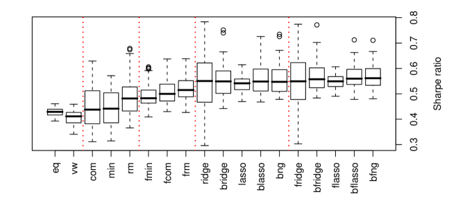
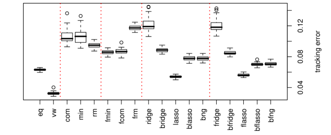
Figure 4: Boxplots of Sharpe ratios (top) and the tracking error (bottom) obtained over 50 random paths through 26 years. The vertical bars correspond to horizontal ones in Table 2.

Figure 4 summarizes the variability in the Monte Carlo experiment showing the distribution (via boxplots) of the Sharpe ratios and tracking error obtained for each of the 50 random paths through the 26 years, thereby complementing the averages presented in Table 2. We can immediately see that the classical ridge regression approach is highly variable, often yielding extremely low Sharpe ratios and high tracking error. The Bayesian approach offers a dramatic improvement here. In the case of the lasso/NG we can see that the variability of the Sharpe ratios for the Bayesian implementations are higher than their classical counterparts. However, it is crucial to observe that the boxplots extend in the direction of larger Sharpe ratios, offering improved estimators.

6 Discussion

We have shown how the classical (MLE/CV) shrinkage approach of Gramacy et al., (2008) to joint multivariate inference under monotone missingness may be treated in a fully Bayesian way to great effect. The Bayesian approach facilitates extensions to deal with “gaps” in the monotone pattern via MDA and heavy-tailed data, and can account for estimation risk. None of these features could be accommodated by the classical approach. In synthetic data experiments we demonstrated the descriptive, predictive, and inferential superiority of the Bayesian methods. Using real financial returns data we showed how the fully Bayesian approach leads to portfolios with lower variability and thus higher Sharpe ratio.

Our methods bear some similarity to other recent approaches to covariance estimation. Levina et al., (2008) and Carvalho and Scott, (2009) offer priors on covariance matrices with shrinkage based on Cholesky decompositions. Our monotone factorization (originally: Andersen,, 1957) can be seen as a special case where the column order, and thus the underlying graphical model structure, is fixed by historical availability. This has certain advantages in our context (relative inferential simplicity, tractability, MDA and heavy tail extensions), but it may not be optimal in complete data cases. Liu, (1996, 1995) provides a model for Bayesian robust multivariate joint inference for data exhibiting a monotone missingness pattern. The posteriors are derived using extensions of Bartlett’s decomposition, and “gaps” may be handled via MDA. Although a wealth of theoretical and empirical results are provided, it is not clear how the methods can be adapted to “big $p$ small $n$” setting. A possible way forward involves Bayesian dynamic factor models (West,, 2003) which are designed for “big $p$ small $n$” and retain the ability to handle missing data in a tractable way.

It is becoming well understood that the Laplace prior has many drawbacks, even when generalized by the NG. For example, it is known to produce biased estimates of the nonzero coefficients and to underestimate of the number of zeros. A newly developed shrinkage prior for regression called the horseshoe (Carvalho et al.,, 2008) shows promise as a tractable alternative (i.e., via GS) without the bias problems. Incorporating horseshoe regression in our framework is part of our future work. Another obvious extension is to relax the i.i.d. assumption to obtain more dynamic estimators. One possible approach might be to use weighted regressions for the $\mathcal{BR}$’s with weights decaying back in time.

Acknowledgments

This work was partially supported by Engineering and Physical Sciences Research Council Grant EP/D065704/1. We would like to thank an anonymous referee, and the associate editor, whose many helpful comments improved the paper.

References

- Andersen, (1957) Andersen, T. (1957). “Maximum Likelihood Estimates for a Multivariate Normal Distribution when Some Observations Are Missing.” J. of the American Statistical Association, 52, 200–203.
- Brown, (1979) Brown, S. (1979). “The Effect of Estimation Risk on Capital Market Equilibrium.” J. of Financial and Quantitative Analysis, 14, 215–220.
- Carlin and Polson, (1991) Carlin, B. P. and Polson, N. G. (1991). “Inference for nonconjugate Bayesian Models using the Gibbs sampler.” The Canadian Journal of Statistics, 19, 4, 399–405.
- Carlin et al., (1992) Carlin, B. P., Polson, N. G., and Stoffer, D. S. (1992). “A Monte Carlo Approach to Nonnormal and Nonlinear State–Space Modeling.” J. of the American Statistical Association, 87, 418, 493–500.
- Carvalho et al., (2008) Carvalho, C., Polson, N., and Scott, J. (2008). “The horseshoe estimator for sparse signals.” Discussion Paper 2008-31, Duke University Department of Statistical Science.
- Carvalho and Scott, (2009) Carvalho, C. M. and Scott, J. G. (2009). “Objective Bayesian model selection in Gaussian graphical models.” Biometrika, asp017.
- Chan et al., (1999) Chan, L. K., Karceski, J., and Lakonishok, J. (1999). “On Portfolio Optimization: Forecasting Covariances and Choosing the Risk Model.” The Review of Financial Studies, 12, 5, 937–974.
- Efron et al., (2004) Efron, B., Hastie, T., Johnstone, I., and Tibshirani, R. (2004). “Least Angle Regression (with discussion).” Annals of Statistics, 32, 2.
- Fama and French, (1993) Fama, E. and French, K. (1993). “Common Risk Factors in the Returns on Stocks and Bonds.” J. of Financial Economics, 33, 3–56.
- George and McCulloch, (1993) George, E. and McCulloch, R. (1993). “Variable selection via Gibbs sampling.” J. of the American Statistical Association, 88, 881–889.
- Geweke, (1992) Geweke, J. (1992). “Priors for microeconomic times series and their application.” Tech. Rep. Institute of Empirical Macroeconomics Discussion Paper No.64, Federal Reserve Bank of Minneapolis.
- Geweke, (1993) — (1993). “Bayesian Treatment of the Independent Student– Linear Model.” J. of Applied Econometrics, Vol. 8, Supplement: Special Issue on Econometric Inference Using Simulation Techniques, S19–S40.
- Geweke, (1996) — (1996). “Variable selection and model comparison in regression.” In Bayesian Statistics 5, eds. J. Bernardo, J. Berger, A. Dawid, and A. Smith, 609–620. Oxford Press.
- Godsill, (2001) Godsill, S. (2001). “On the relationship between Markov chain Monte Carlo methods for model uncertainty.” J. of Computational and Graphical Statistics, 10, 2, 239–248.
- Gramacy, (2009) Gramacy, R. B. (2009). The monomvn package: Estimation for multivariate normal and Student-t data with monotone missingness. R package version 1.8.
- Gramacy et al., (2008) Gramacy, R. B., Lee, J. H., and Silva, R. (2008). “On estimating covariances between many assets with histories of highly variable length.” Tech. Rep. 0710.5837, arXiv. Url: http://arxiv.org/abs/0710.5837.
- Green, (1995) Green, P. (1995). “Reversible Jump Markov Chain Monte Carlo Computation and Bayesian Model Determination.” Biometrika, 82, 711–732.
- Griffin and Brown, (2010) Griffin, J. E. and Brown, P. J. (2010). “Inference with Normal–Gamma prior distributions in regression problems.” Bayesian Analysis, 1, 5, 171–188.
- Hans, (2008) Hans, C. (2008). “Bayesian lasso regression.” Tech. Rep. 810, Department of Statistics, The Ohio State University, Columbus, OH 43210.
- Hastie et al., (2001) Hastie, T., Tibshirani, R., and Friedman, J. (2001). The Elements of Statistical Learning: Data Mining, Inference, and Prediction. Springer.
- Hoerl and Kennard, (1970) Hoerl, A. and Kennard, R. (1970). “Ridge Regression: Biased estimation for non-orthogonal problems.” Technometrics, 12, 55–67.
- Jacquier et al., (2004) Jacquier, E., Polson, N., and Rossi, P. E. (2004). “Bayesian analysis of stochastic volatility models with fat-tails and correlated errors.” J. of Econometrics, 122, 185–212.
- Jagannathan and Ma, (2003) Jagannathan, R. and Ma, T. (2003). “Risk Reduction in Large Portfolios: Why Imposing the Wrong Constraints Helps.” J. of Finance, 58, 4, 1641–1684.
- Klein and Bawa, (1976) Klein, R. and Bawa, V. (1976). “The Effect of Estimation Risk on Optimal Portfolio Choice.” J. of Financial Econometrics, 3, 215–231.
- Ledoit and Wolf, (2002) Ledoit, O. and Wolf, M. (2002). “Improved estimation of the covariance matrix of stock returns with an application to portfolio selection.” J. of Emperical Finance, 10, 603–621.
- Levina et al., (2008) Levina, E., Rothman, A., and Zhu, J. (2008). “Sparse Estimation of Large Covariance Matrices via a Nested Lasso Penalty.” Annals of Applied Statistics, 2, 1, 245–263.
- Li, (1988) Li, K. (1988). “Imputation using Markov chains.” J. of Statistical Computation, 30, 57–79.
- Little and Rubin, (2002) Little, R. J. and Rubin, D. B. (2002). Statistical Analysis with Missing Data. 2nd ed. Wiley.
- Liu, (1993) Liu, C. (1993). “Bartlett’s decomposition of the posterior distribution of the covariance for normal monotone ignorable missing data.” J. of Multivariate Analysis, 46, 198–206.
- Liu, (1995) — (1995). “Monotone Data Augmentation Using the Multivariate Distribution.” J. of Multivariate Analysis, 53, 139–158.
- Liu, (1996) — (1996). “Bayesian Robust Multivariate Linear Regression With Incomplete Data.” J. of the American Statistical Association, 91, 435, 1219–1227.
- Markowitz, (1959) Markowitz, H. (1959). Portfolio Selection: Efficient Diversification of Investments. New York: John Wiley.
- Park and Casella, (2008) Park, T. and Casella, G. (2008). “The Bayesian Lasso.” J. of the American Statistical Association, 103, 482, 681–686.
- Polson and Tew, (2000) Polson, N. and Tew, B. (2000). “Bayesian Portfolio Selection: An Empirical Analysis of the S&P 500 Index 1970–1996.” J. of Business & Economic Statistics, 18, 2, 164–173.
- Schafer, (1997) Schafer, J. (1997). Analysis of Incomplete Multivariate Data. Chapman & Hall/CRC.
- R Development Core Team, (2007) R Development Core Team (2007). R: A Language and Environment for Statistical Computing. R Foundation for Statistical Computing, Vienna, Austria. ISBN 3-900051-07-0.
- Stambaugh, (1997) Stambaugh, R. F. (1997). “Analyzing Investments Whose Histories Differ in Lengh.” J. of Financial Economics, 45, 285–331.
- Tibshirani, (1996) Tibshirani, R. (1996). “Regression Shrinkage and Selevtion via the Lasso.” J. of the Royal Statistical Society, Series B, 58, 267–288.
- Troughton and Godsill, (1997) Troughton, P. T. and Godsill, S. J. (1997). “A reversible jump sampler for autoregressive time series, employing full conditionals to achieve efficient model space moves.” Tech. Rep. CUED/F-INFENG/TR.304, Cambridge University Engineering Department.
- West, (2003) West, M. (2003). “Bayesian factor regression models in the “large , small ” paradigm.” Bayesian Statistics 7, 723–732.
- Zellner and Chetty, (1965) Zellner, A. and Chetty, V. (1965). “Prediction and Decision Problems in Regression Models From the Bayesian Point of View.” J. of the American Statistical Association, 605–616.