Functional renormalization group approach to the BCS-BEC crossover

Abstract

The phase transition to superfluidity and the BCS-BEC crossover for an ultracold gas of fermionic atoms is discussed within a functional renormalization group approach. Non-perturbative flow equations, based on an exact renormalization group equation, describe the scale dependence of the flowing or average action. They interpolate continuously from the microphysics at atomic or molecular distance scales to the macroscopic physics at much larger length scales, as given by the interparticle distance, the correlation length, or the size of the experimental probe. We discuss the phase diagram as a function of the scattering length and the temperature and compute the gap, the correlation length and the scattering length for molecules. Close to the critical temperature, we find the expected universal behavior. Our approach allows for a description of the few-body physics (scattering and molecular binding) and the many-body physics within the same formalism.

I Introduction

The binding energy of molecules formed from two fermionic atoms may depend on external parameters such as a magnetic field $B$. We discuss a gas of two degenerate species of atoms (typically hyperfine states), where bound molecules form for $B<B_{0}$, whereas for $B>B_{0}$ only unstable resonance states are present. At the Feshbach resonance $B=B_{0}$, the scattering length $a$ diverges. At low temperatures $T$ and for large $B-B_{0}$, the molecules play no role and one expects superfluidity of the BCS type BCS . In the opposite case of large negative $B-B_{0}$, the bosonic molecules dominate at low temperatures $T$ and Bose-Einstein condensation (BEC) BoseEinstein should occur. In the vicinity of the Feshbach resonance, a continuous crossover from BCS to BEC condensation has been predicted p5ALeggett80 . Several recent experiments have established this overall picture Exp . In parallel, a considerable theoretical effort has been devoted to a quantitatively precise theoretical understanding of this phenomenon Nussinov ; Nishida:2006br ; Nishida:2006eu ; EpsilonExpansion ; Nikolic:2007zz ; AbukiBrauner ; MonteCarlo ; MonteCarloBulgac ; MonteCarloBuro ; MonteCarloAkki ; TMatrix ; Diehl:2005ae ; Diener08 ; Haussmann:2007zz ; Birse05 ; Diehl:2007th ; Diehl:2007XXX ; Gubbels:2008zz ; FSDW08 ; KopLo09 .

A major motivation for the theoretical effort is due to the possibility of using this system as a testing ground for non-perturbative methods in many-body theory, which go beyond the mean-field approximation. Quantitatively reliable methods for complex many-body systems are crucial for many areas in physics, from condensed matter phenomena to nuclear or elementary particle physics. For a non-relativistic system, as in our case, the results of such methods may be tested, in principle, by a huge number of experiments and observations. However, for a quantitatively precise test the underlying microphysics must be known with sufficient precision. This is often not the case for real physical systems in condensed matter physics. A notable exception is the universal physics near a second order phase transition, where the critical exponents and amplitude ratios no longer depend on microscopic details. The quantitative computations of these universal quantities by the renormalization group has been one of the major breakthroughs in theoretical physics Wilson ; Wegner .

In cold atom gases, the microscopic physics is well under control, since it can be directly related to atomic and molecular properties and measured by scattering experiments. This gives rise to the hope that experimental tests become now available for the whole connection between microphysics on the one and the macroscopic quantities as thermodynamics, condensation phenomena, the correlation length, defects etc. on the other side. Furthermore, the effective strength of interaction can be tuned experimentally, which offers the fascinating perspective of following the tests of theoretical methods from the well-controlled perturbative domain for small scattering length to the difficult non-perturbative region for large scattering length.

First results for the BCS-BEC crossover are now available for a number of theoretical methods that go beyond mean-field theory. Quantitative understanding of the crossover at and near the resonance has been developed through numerical calculations using various quantum Monte-Carlo (QMC) methods MonteCarlo ; MonteCarloBulgac ; MonteCarloBuro ; MonteCarloAkki . Computations of the complete phase diagram have been performed from functional field-theoretical techniques, in particular from $\epsilon$-expansion Nussinov ; Nishida:2006br ; Nishida:2006eu ; EpsilonExpansion , $1/N$-expansion Nikolic:2007zz ; AbukiBrauner , $t$-matrix approaches TMatrix , Dyson-Schwinger equations Diehl:2005ae ; Diener08 , 2-Particle Irreducible methods Haussmann:2007zz , and renormalization-group flow equations Birse05 ; Diehl:2007th ; Diehl:2007XXX ; Gubbels:2008zz ; FSDW08 ; KopLo09 .

In this paper, we give an account of the functional renormalization group approach for the BCS-BEC crossover which is based on the flowing action (or average action) Wetterich:1992yh . We concentrate here on the detailed description of the formalism which underlies the results presented in ref. Diehl:2007th ; Diehl:2007XXX ; FSDW08 . Furthermore, we extend the results of these papers by results for the correlation length and the self-interaction of the bosonic molecules, including the behavior near the phase transition.

Our paper is organized as follows. Sect. II focuses on the method which we use in order to tackle the crossover problem, the functional renormalization group. Our starting point is an exact functional renormalization group equation for the average potential Wetterich:1992yh . We specify the approximation scheme used for our practical computations and present the non-perturbative flow equations. Details and various quantities needed for a numerical solution can be found in a series of appendices A-F. This section provides the technical basis for our work.

The physics of the crossover problem is addressed in the following sections. It can be structured into two parts: Few-body and many-body problem. In our formalism, both parts find a unified description. In Sect. III we discuss the phase transition to superfluidity at low $T$ within our formalism. We present results for the temperature dependence of the gap and the correlation length for $T\leq T_{\mathrm{c}}$. For a comparison with experiment, we need to relate the microscopic parameters appearing in the microscopic action to physical observables as the scattering length or the molecular binding energy. The latter quantities concern the behavior of a two-atom system. In our formalism, this can be described as the vacuum limit where density and temperature approach zero. This is discussed in Sect. IV. Sect. V extends the simplest truncation (discussed in Sect. II) in order to include the particle-hole fluctuations FSDW08 . In Sect. VI, we demonstrate the capacity of the model to incorporate directly the universal critical physics at the phase transition. We discuss the behavior of the scattering length for molecules as the critical temperature is approached. In Sect. VII we address the question of a quantitatively precise computation of the density. The density sets the only scale in the unitarity limit where the scattering length for atoms diverges. It enters directly the theoretical predictions as the ratio $T_{\mathrm{c}}/T_{\mathrm{F}}$, where the Fermi temperature $T_{\mathrm{F}}$ is given by the density. The determination of the density by a direct computation of the thermodynamic potential on the chemical potential $\mu$ leads to a lower value than the “free particle density”. As a result, the value of $T_{\mathrm{c}}/T_{\mathrm{F}}$ is somewhat higher. We present conclusions in Sect. VIII.

II Functional Renormalization

II.1 Effective Action and Potential

We express our microscopic model in terms of the action

$$S[\varphi,\psi]=\int_{0}^{\beta}d\tau\int d^{3}x\Bigl{(}\psi^{\dagger}\left(\partial_{\tau}-\Delta-\mu\right)\psi$$

$$\hskip 34.14322pt+\varphi^{*}\left(\partial_{\tau}-\frac{1}{2}\Delta+\nu-2\mu\right)\varphi$$

$$\hskip 34.14322pt-\frac{h_{\varphi}}{2}\left(\varphi^{*}\psi^{T}\epsilon\psi-\varphi\psi^{\dagger}\epsilon\psi^{*}\right)\Bigr{)}\,,$$ (1)

where $\psi^{T}\epsilon\psi=2\psi_{1}\psi_{2}$, $\psi^{\dagger}\epsilon\psi^{*}=2\psi_{1}^{*}\psi_{2}^{*}$ and $\triangle$ is the Laplacian. This model describes nonrelativistic fermions in two different states, a composite bosonic field and a Yukawa type interaction between them. We represent the fermion field by the complex two-component spinor $\psi=(\psi_{1},\psi_{2})$ ($\epsilon$ is the totally antisymmetric symbol) and the bosonic complex scalar field by $\varphi$. Depending on the situation, $\varphi$ can describe a bound state of two fermions (molecule), the closed channel state of a Feshbach resonance or a Cooper-pair like collective state of two fermions. As long as its dynamics plays no role, it can also be considered as an auxiliary field that is used as an effective parameterization of a purely fermionic interaction.

We work with the formalism of quantum statistics in the grand canonical ensemble with chemical potential $\mu$. In addition to the spatial position $\vec{x}$, the fields depend on Euclidean time $\tau$. At nonzero temperature, this Euclidean time is wrapped around a torus of circumference $\beta=\frac{1}{T}$. This implies for the boson field $\varphi(\vec{x},\beta)=\varphi(\vec{x},0)$, while the fermion field gets an additional minus sign due to its Grassmann property $\psi(\vec{x},\beta)=-\psi(\vec{x},0)$. Here, and in the following we choose our units such that $\hbar=k_{\mathrm{B}}=1$. In addition, we also rescale time, and the fields in units of the fermion mass $M$ such that effectively $2M=1$. App. A gives a brief summary how eV units for the physical observables are recovered from our units.

At tree level, the Yukawa term leads to an effective four fermion interaction $\psi_{1}\,\psi_{2}\rightarrow\psi^{\dagger}_{1}\,\psi^{\dagger}_{2}$, with coupling strength

$$\lambda_{\psi,\text{eff}}=-\frac{h_{\varphi}^{2}}{\nu-2\mu+iq_{0}+\frac{1}{2}\vec{q}^{2}}.$$ (2)

Here, $q_{0}$ and $\vec{q}$ denote the center of mass Euclidean frequency and momentum of the scattering particles $\psi_{1}$ and $\psi_{2}$. The real time frequency $\omega$ obtains by analytic continuation, $iq_{0}\to-\omega$, such that the microscopic dispersion relation for the molecules is $\omega=\vec{q}^{2}/2+\nu-2\mu$. In the limit $h^{2}_{\varphi}\to\infty,\nu\to\infty,h^{2}_{\varphi}/\nu\to~{}\text{const.}$ one can neglect $q_{0},\vec{q}^{2}$ and $\mu$ in Eq. (1), such that the effective fermionic interaction becomes pointlike, cf. Diehl:2005ae and Sect. IV.3.

Our aim is the computation of the quantum effective action $\Gamma[\varphi,\psi]$. It has a structure similar to the microscopic action $S$, but with microscopic couplings and fields replaced by renormalized macroscopic couplings and fields. Furthermore, the couplings will depend on momentum, and $\Gamma$ contains additional couplings not present in $S$. The quantum effective action generates the one-particle-irreducible vertices (amputated scattering vertices) and (inverse) full propagators. The field equations derived from an extremum principle for $\Gamma$ are exact equations - all contributions from quantum and thermal fluctuations are included. All scattering information can be easily extracted from $\Gamma$ as well as all thermodynamic relations.

For constant scalar fields $\varphi(\vec{x},\tau)=\varphi$ and $\psi(\vec{x},\tau)=0$, the effective action reduces to the effective potential $U(\varphi)$, since $\Gamma=(V_{3}/T)U(\varphi)$ with $V_{3}$ being the volume. The $U(1)$ symmetry of global phase rotations implies that $U$ can only depend on the invariant $\rho=\varphi^{*}\varphi$. The field equation $\partial U/\partial\varphi=0$ determines the location $\varphi_{0}$ of the minimum of $U$. Any nonzero $\varphi_{0}$ amounts to a spontaneous breaking of the $U(1)$ symmetry. The associated Goldstone boson is responsible for superfluidity. Therefore, $\varphi_{0}$ is an order parameter – more precisely, $2\rho_{0}=2\varphi^{*}_{0}\varphi_{0}$ is the superfluid density. The system is in the superfluid phase if $\rho_{0}(T,\mu)>0$, and in the disordered or symmetric phase if $\rho_{0}(T,\mu)=0$. The knowledge of $U(\rho;T,\mu)$ thus permits a straightforward extraction of the phase diagram. Furthermore, the value of $U$ at the minimum corresponds to the pressure

$$p(T,\mu)=-U(\rho_{0};T,\mu).$$ (3)

(We choose a free additive constant in $U$ such that $p(0,0)=0.)$ The grand potential or Landau thermodynamic potential $\Phi_{G}$ is related to $U(\rho_{0})$ by

$$\Phi_{G}=V_{3}U(\rho_{0}),$$ (4)

and we obtain the usual relations for the particle density $n$, entropy density $s$ and energy density $\epsilon$:

$$n = \frac{\partial p}{\partial\mu}{\bigg{|}}_{T}=-\frac{\partial U}{\partial\mu}(\rho_{0}),$$

$$s = \frac{\partial p}{\partial T}{\bigg{|}}_{\mu}=-\frac{\partial U}{\partial T}(\rho_{0}),$$

$$\epsilon = -p+Ts+\mu n=U(\rho_{0})+Ts+\mu n.$$ (5)

II.2 Flow equation for the average potential

The effective potential $U$ contains all the essential information for the description of the equilibrium properties of a homogeneous system. Its computation is, however, a challenge, since quantum and thermal fluctuations on all momentum scales have to be computed. The average potential $U_{k}$ includes only the effects of bosonic fluctuations with momenta $\vec{q}^{2}>k^{2}$ and fermionic fluctuations with $|\vec{q}^{2}-p_{\mathrm{F}}^{2}|>k^{2}$, with $p_{\mathrm{F}}$ the Fermi momentum. It is therefore a type of coarse-grained free energy. If $k$ is large enough, the complicated infrared physics for bosons and physics close to the Fermi surface for fermions is not yet included, and one expects that the complexity of the problem is reduced. In the limit $k\to\infty$, no fluctuation effects are included at all, and the average potential becomes the classical potential extracted from (1),

$$U_{k\to\infty}(\rho)=U_{\text{cl}}(\rho)=(\nu-2\mu)\rho,\quad\rho=\varphi^{\ast}\varphi.$$ (6)

On the other hand, for $k\to 0$ all fluctuation effects are included and $U_{k=0}$ equals the effective potential $U$. The challenge therefore is to construct an interpolation from the microscopic potential $U_{k\to\infty}$ to the effective potential $U_{k\to 0}$.

The dependence of $U_{k}$ on the “average scale” $k$ obeys an exact renormalization group equation or flow equation Diehl:2007th , with $q=(\omega,\vec{q})$

$$\partial_{k}U_{k}(\varphi) = \frac{1}{2}\int_{q}\Big{\{}\text{tr}_{\varphi}[\bar{G}^{-1}_{\varphi}(\varphi;q)+R^{(\varphi)}_{k}(q)]^{-1}\partial_{k}R^{(\varphi)}_{k}(q)$$

$$-\text{tr}_{\psi}[G^{-1}_{\psi}(\varphi;q)+R^{(\psi)}_{k}(q)]^{-1}\partial_{k}R^{(\psi)}_{k}(q)\Big{\}}.$$

Figure 1: Flow of the effective action in the space of couplings. The flow starts at an initial scale $\Lambda$, where all fluctuations are suppressed and the effective action reduces to the classical action. By solving the FRG equations we follow the flow in parameter space down to $k=0$. Two-body scattering observables are measured in the physical vacuum defined as the state with $n=T=0$, but at $k=0$ – all vacuum fluctuations are included. The classical action at $k=\Lambda$ is chosen such as to match the two-body observables in the physical vacuum state (dashed line). We then switch on temperature and density to solve the many-body problem. The many-body flow deviates from the vacuum flow when the cutoff wavelength $k^{-1}$ becomes comparable to the characteristic thermodynamic wavelengths, i.e. the de Broglie wavelength $\lambda_{\text{dB}}\sim T^{-1/2}$ and the mean interparticle spacing $d\sim n^{-1/3}$ (solid line).

The first piece accounts for the bosonic fluctuation and the second for the fermions. Eq. (II.2) is an exact functional differential equation. It includes all orders in a perturbative expansion as well as all non-perturbative effects.

In order to understand the structure of this equation we first include only the bosonic contribution. Our model reduces in this case to a gas of bosons, for which the flow equations FloerchingerWetterich and thermodynamics FWThermod have been discussed extensively in presence of a repulsive interaction and for arbitrary dimension. In Eq. (II.2) we encounter the propagator $\bar{G}_{\varphi}$ of the scalar field in an arbitrary background $\varphi$. We use a two-component basis of real fields $\varphi_{1},\varphi_{2}$, related to the complex field by $\varphi(x)=\frac{1}{\sqrt{2}}\big{(}\varphi_{1}(x)+i\varphi_{2}(x)\big{)}$. Correspondingly, $\bar{G}^{-1}_{\varphi}$ is a $2\times 2$ matrix and $\text{tr}_{\varphi}$ denotes the trace in this space. In the classical approximation, the inverse propagator reads

$$\bar{G}^{-1}_{\varphi,\text{cl}}=\left(\begin{array}[]{ccc}\vec{q}^{2}/2+\nu-2\mu&-q_{0}\\ q_{0}&\vec{q}^{2}/2+\nu-2\mu\end{array}\right).$$ (8)

In the absence of an interaction between the bosons, it is independent of $\varphi$. For $\nu=2\mu$, the classical propagator $\bar{G}_{\varphi,cl}$ becomes singular for $q=(q_{0},\vec{q})\to 0$. It is regularized by adding a momentum-dependent infrared cutoff $R^{(\varphi)}_{k}(q)$ (a unit matrix in $\varphi_{1},\varphi_{2}$ space) which has the general properties

$$\lim_{\frac{k^{2}}{q^{2}}\to\infty}R_{k}(q)\sim k^{2} \lim_{\frac{k^{2}}{q^{2}}\to\ 0}R_{k}(q)\to 0.$$ , (9)

For $k>0$ the combination $(\bar{G}_{\varphi}^{-1}+R_{k}^{(\varphi)})^{-1}$ remains finite even for $\vec{q}^{2}/2+\nu-2\mu=0$. In principle, Eq. (II.2) holds for arbitrary cutoff functions $R_{k}(q)$ that fulfill Eq. (9). For approximate solutions of Eq. (II.2) an appropriate choice is important, however, and we discuss our choice of $R_{k}$ in App. C.

The structure of the flow equation (II.2) already becomes clear in a perturbative one loop truncation: if we replace $\bar{G}_{\varphi}$ by $\bar{G}_{\varphi,\text{cl}}$ in the flow equation, the inverse propagator is independent of $k$ such that the $k$ integration can be performed analytically

$$U_{k}=U_{\text{cl}}+\frac{1}{2}\int_{q_{0}}\int_{\vec{q}}\text{tr}_{\varphi}\ln[\bar{G}^{-1}_{\varphi}+R_{k}].$$ (10)

With $\int_{\vec{q}}=\int d^{3}\vec{q}/(2\pi)^{3},~{}\int_{q_{0}}=T\sum_{n},~{}q_{0}=2\pi nT$, we recognize the regularized one-loop contribution. For $k=0$ and $\nu=2\mu$, one rediscovers the pressure of a gas of free bosons. For $T<T_{\text{c}}$, this describes Bose-Einstein condensation.

The exact flow equation is obtained if we perform a “renormalization group improvement” of the propagator and replace in Eq. (II.2) the classical inverse propagator by the full inverse propagator in the presence of a “background field” $\varphi$. The full inverse propagator is given by the second functional derivative of the average action $\Gamma_{k}$ with respect to the background fields $\varphi(x)$. This average action generalizes the effective potential in the presence of derivative terms for the fields. We will discuss this in more detail below. What is important at this stage is that $\bar{G}_{\varphi}^{-1}$ typically depends on $\varphi$, thus generating a non-trivial $\varphi$-dependence in the flow equation (II.2). Indeed, in the presence of effective bosonic interactions $\Gamma_{k}$ will not be quadratic in $\varphi$ anymore.

If one neglected the $k$-dependence of $\bar{G}_{\varphi}^{-1}$, Eq. (10) would give the one-loop perturbative result for interacting bosons. However, beyond this approximation $\bar{G}_{\varphi}^{-1}$ will depend on $k$ since only fluctuations with momenta $\vec{q}^{2}>k^{2}$ are included in its computation. Then Eq. (II.2) becomes a non-linear differential equation that has to be solved numerically. Nevertheless, its structure always remains a one-loop equation with only one momentum integration. The only difference from one loop perturbation theory arises from the use of the full field and momentum dependent propagator. Higher (perturbative) loops as well as non-perturbative effects are created due to the non-linear nature of the flow equation.

In the BEC-limit the fermion chemical potential $\mu$ assumes negative values, as appropriate for a gas of bosons. Starting from the action in Eq. (1) we could perform the Gaussian functional integral for the fermions, resulting in an effective action involving only the bosonic field $\varphi$. In general, the effective bosonic action is a complicated non-local object. However, for large enough negative $\mu$ (as compared to the typical frequencies $\omega$ and kinetic energies $\vec{q}^{2}/2$) the bosonic action becomes effectively local. We could then use the purely bosonic flow equation, starting with a non-polynomial classical potential $U_{\Lambda}(\varphi)$. We therefore expect to recover in the BEC-limit many features of a boson gas with repulsive interactions. (There may be quantitative differences as compared to the case of a pointlike interaction between two bosons, due to the non-polynomial $U(\varphi)$ which also depends on $\mu$.)

Away from the BEC-limit the fermion fluctuations will play a crucial role – they dominate in the BCS-limit. We therefore have to solve the full Eq. (II.2). The fermionic contribution in Eq. (II.2) is of a similar nature as the bosonic contribution, with the characteristic minus sign for a fermion loop and $G^{-1}_{\psi}$ being the full fermionic inverse propagator. The fermionic cutoff $R^{(\psi)}_{k}$ is chosen such that it regularizes the momenta close to the Fermi surface rather than the small momenta, see App. C.

The BCS limit obtains for $\mu>0$ and large positive $\nu$ and $h_{\varphi}^{2}/\nu$. The qualitative features can now be understood in the limit where the boson fluctuations can be neglected. The inverse fermion propagator $G_{\psi}^{-1}$ will contain a piece $\sim h_{\varphi}\varphi$ due to the Yukawa interaction in Eq. (1). This induces contributions to the effective potential $U(\varphi)$, which lead to a minimum away from $\varphi=0$ if the temperature is low enough. In the classical approximation the fermion inverse propagator reads

$$G^{-1}_{\psi}=\left(\begin{array}[]{ccc}-h_{\varphi}\epsilon\varphi^{\ast}&&iq_{0}-(\vec{q}\,^{2}-\mu)\\ iq_{0}+\vec{q}\,^{2}-\mu&&h_{\varphi}\epsilon\varphi\end{array}\right).$$ (11)

This is a $4\times 4$ matrix, where we have suppressed the spinor indices. (The symbol $\epsilon_{\alpha\beta}$ acts on the spinor indices $\alpha=1,2$.) In the limit where the $k$-dependence of $h_{\varphi}$ is neglected we can again integrate in order to obtain the one loop result for $k=0$

$$U_{0}(\varphi) = U_{\text{cl}}(\varphi)-\frac{1}{2}\int_{q_{0}}\int_{\vec{q}}\text{tr}_{\psi}\ln G_{\psi}^{-1}$$

$$= (\nu_{\Lambda}-2\mu)\varphi^{*}\varphi$$

$$- 2T\int_{\vec{q}}\ln\left[\text{cosh}\left(\sqrt{(\vec{q}^{2}-\mu)^{2}+h_{\varphi}^{2}\varphi^{*}\varphi}/2T\right)\right].$$

Condensation occurs if the minimum of $U_{0}$ occurs for $|\varphi_{0}|>0$. This always happens for small enough temperature $T$. Determining from Eq. (11) the critical temperature $T_{\mathrm{c}}$ for the onset of a condensate $\varphi_{0}\neq 0$ yields the BCS value. (For this purpose we relate $\nu_{\Lambda}$ to the scattering length $a$ in Sect. IV.) For quantitative accuracy the bosonic fluctuations cannot be neglected even deep in the BCS region. We will see in Sect. V that they induce in our formalism the corrections from the particle-hole fluctuations.

From Eq. (II.2) we can read off the fermion dispersion $E_{\vec{q}}=\sqrt{(\vec{q}^{2}-\mu)^{2}+h_{\varphi}^{2}\varphi^{*}_{0}\varphi_{0}}$. Thus, $\Delta=h_{\varphi}\varphi_{0}$ represents the $U(1)$ symmetry breaking mass term or gap for the single particle excitations. In our framework, it is proportional to the bosonic field expectation value, such that spontaneous symmetry breaking $\rho_{0}=\varphi_{0}^{*}\varphi_{0}\neq 0$ and a gap for the fermions coincide. The actual values of $h_{\varphi},\rho_{0}$ are, however, determined beyond the mean field approximation, cf. e.g. Eq. (II.4).

II.3 Truncation

The full propagators $G_{\varphi,\psi}$ remain complicated objects. It is at this level that we need to proceed with an approximation by making an ansatz for their general form. This amounts to a truncation of the most general form of the average action $\Gamma_{k}$, which is the generalization of the average potential $U_{k}$ to a functional of space- and time-dependent fields $\varphi(x),\psi(x)$. In other words, $\Gamma_{k}$ is the quantity corresponding to the effective action $\Gamma$ in the presence of the infrared cutoff $R_{k}$, which suppresses the fluctuation effects arising from momenta $\vec{q}^{2}<k^{2}$.

A truncation of $\Gamma_{k}$ should respect the symmetries, which we discuss in App. B. Since fluctuations for the derivative terms will turn out to be important for the composite bosonic field we have to distinguish carefully between microscopic (bare) and renormalized fields and couplings. We use in this paper the lowest order in a derivative expansion which, in terms of bare quantities, reads

$$\Gamma_{k} = \int_{\tau,\vec{x}}\Big{\{}\bar{U}_{k}(\bar{\rho})+\bar{\varphi}^{\ast}(Z_{\varphi}\partial_{\tau}-\frac{1}{2}A_{\varphi}\Delta)\bar{\varphi}$$

$$+\psi^{\dagger}(\partial_{\tau}-\Delta-\mu)\psi-\frac{\bar{h}_{\varphi}}{2}(\bar{\varphi}^{\ast}\psi^{T}\epsilon\psi-\bar{\varphi}\psi^{\dagger}\epsilon\psi^{\ast})\Big{\}}.$$

The bar denotes bare fields and couplings, which can be related to renormalized quantities by absorbing the running gradient coefficient $A_{\varphi}$ by a field rescaling $\varphi=A_{\varphi}^{1/2}\bar{\varphi}$ (wavefunction renormalization). As we neglect the fermionic wave function renormalization in this work, there is no need to distinguish between bare and renormalized fermion fields here. In terms of renormalized fields, the truncation then reads

$$\Gamma_{k} = \int_{\tau,\vec{x}}\Big{\{}U_{k}(\rho)+\varphi^{\ast}(S_{\varphi}\partial_{\tau}-\frac{1}{2}\Delta)\varphi$$

$$+\psi^{\dagger}(\partial_{\tau}-\Delta-\mu)\psi-\frac{h_{\varphi}}{2}(\varphi^{\ast}\psi^{T}\epsilon\psi-\varphi\psi^{\dagger}\epsilon\psi^{\ast})\Big{\}}.$$

with the renormalized couplings $S_{\varphi}=Z_{\varphi}/A_{\varphi}$, $h_{\varphi}=\bar{h}_{\varphi}/\sqrt{A_{\varphi}}$, order parameter $\rho=A_{\varphi}\bar{\rho}$, and effective potential $U(\rho)=\bar{U}(\bar{\rho})$. In addition to the average potential $\bar{U}_{k}$, the wave function renormalizations $Z_{\varphi},A_{\varphi}$ and the Yukawa coupling $\bar{h}_{\varphi}$ depend on $k$. In this approximation the renormalized inverse boson propagator $G_{\varphi}^{-1}=\bar{G}_{\varphi}^{-1}/A_{\varphi}$ reads

$$G^{-1}_{\varphi} = \left(\begin{array}[]{ccc}U^{\prime}_{k}+2\rho U^{\prime\prime}_{k}+\vec{q}\,^{2}/2&&-S_{\varphi}q_{0}\\ S_{\varphi}q_{0}&&U^{\prime}_{k}+\vec{q}^{2}/2\end{array}\right).$$ (17)

Here, primes denote derivatives with respect to $\rho$. The fermionic inverse propagator is given in Eq. (11), where we use a basis $(\psi,\psi^{\ast})$.

We emphasize that $U_{k}$ appears on the right-hand side of Eq. (II.2): at any given scale $k$ the flow is determined by the average potential $U_{k}$ at the same scale $k$ rather than by the classical potential. The same holds for the $k$-dependent Yukawa coupling $h_{\varphi}$. The right-hand side of the flow equation is only sensitive to the physics at the scale $k$. In particular, the structure of the flow equations implies that the momentum integrals in Eq. (II.2) are dominated by a small range $\vec{q}^{2}\approx k^{2}$. This is the main reason why a derivative expansion often works rather well. In principle, $A_{\varphi},Z_{\varphi}$ and $h_{\varphi}$ are momentum-dependent functions. If this momentum dependence is not too strong, and the effective range of momenta in the integral (II.2) remains rather small, a momentum-independent approximation is a good starting point. The truncation Eq. (II.3) forms the basis for the results presented in this paper. A similar truncation has been advocated for attractive fermions on the lattice in Ref. Strack08 . In Sect. V we extend it to assess the effect of particle-hole fluctuations.

The truncation in Eq. (II.3) has been extended in ref. FSW10 where renormalization effects on the fermionic self-energy and in particular a wavefunction renormalization factor for the fermions have been included. For a detailed discussion we refer to ref. FSW10 .

II.4 Non-perturbative flow equation

Figure 2: Diagrammatic representation of the flow equations for bare quantities in the symmetric phase. The flow of the inverse propagator is displayed in the first line. The frequency and momentum dependence of the loops is projected according to Eqs. (II.4). The fermionic graph, present in the mean-field treatment taking Gaussian bosonic fluctuations into account, is supplemented with a feedback of bosonic fluctuations due to the second graph. These effects are important to capture the expected long-wavelength behavior close to the second-order phase transition, whereas this graph vanishes in the physical vacuum $n=T=0$. The Yukawa vertex in the second line does not flow within our truncation due the $U(1)$ symmetry. This changes in extended truncations FSDW08 . Moreover, in the symmetry-broken phase the flow equations become more complex, due to processes describing scattering off the condensate. In this case, also the Yukawa vertex acquires a nonzero flow. The $\tilde{\partial}_{t}$ derivative acts on the cutoff functions in the regularized propagators only.

For our choice of $R_{k}$ and with the approximation (17), we can perform the momentum integration and the Matsubara sums explicitly

$$k\partial_{k}U_{k} = \eta_{A_{\varphi}}\,\rho\,U^{\prime}_{k}+\frac{\sqrt{2}k^{5}}{3\pi^{2}S_{\varphi}}\left(1-2\eta_{A_{\varphi}}/5\right)s_{\mathrm{B}}^{(0)}$$ (18)

$$-\frac{k^{5}}{3\pi^{2}}\,l(\tilde{\mu})\,s_{\mathrm{F}}^{(0)},$$

$$l(\tilde{\mu}) = \left(\theta(\tilde{\mu}+1)(\tilde{\mu}+1)^{3/2}-\theta(\tilde{\mu}-1)(\tilde{\mu}-1)^{3/2}\right).$$

Here we use the dimensionless chemical potential $\tilde{\mu}=\mu/k^{2}$, the ratio $S_{\varphi}=Z_{\varphi}/A_{\varphi}$ and the anomalous dimension $\eta_{A_{\varphi}}=-\partial\text{ln}A_{\varphi}/\partial\text{ln}k$. The threshold functions $s_{\mathrm{B}}$ and $s_{\mathrm{F}}$ depend on $w_{1}=U_{k}^{\prime}/k^{2}$, $w_{2}=(U_{k}^{\prime}+2\rho U_{k}^{\prime\prime})/k^{2}$, $w_{3}=h^{2}_{\varphi}\rho/k^{4}$, as well as on the dimensionless temperature $\tilde{T}=T/k^{2}$. They describe the decoupling of modes if the effective “masses” or “gaps” $w_{j}$ get large. They are normalized to unity for vanishing arguments and $\tilde{T}\to 0$ and read

$$s_{B}^{(0)} = \left[\sqrt{\frac{1+w_{1}}{1+w_{2}}}+\sqrt{\frac{1+w_{2}}{1+w_{1}}}\right]$$

$$\times\left[\frac{1}{2}+N_{\mathrm{B}}(\sqrt{1+w_{1}}\sqrt{1+w_{2}}/S_{\varphi})\right],$$

$$s_{\text{F}}^{(0)} = \frac{2}{\sqrt{1+w_{3}}}\left[\frac{1}{2}-N_{\mathrm{F}}(\sqrt{1+w_{3}})\right].$$ (19)

(For $s_{\mathrm{B}}^{(0)}$, only all its $\rho$ derivatives vanish for $w_{1}\sim w_{2}\to\infty$. The remaining constant part is a shortcoming of the particular choice of the cutoff acting only on spacelike momenta.)

In Eq. (II.4) the temperature dependence arises through the Bose and Fermi functions

$$N_{B/F}(\epsilon)=\frac{1}{e^{\epsilon/\tilde{T}}\mp 1}.$$ (20)

For $\tilde{T}\to 0$ the “‘thermal parts” $\sim N_{\mathrm{B,F}}$ vanish, whereas for large $\tilde{T}$ one has

$$s_{\mathrm{F}}^{(0)}\to\tilde{T}^{-1},\quad s_{\mathrm{B}}^{(0)}\to 2\tilde{T}S_{\varphi}(1+w_{1})^{-1}(1+w_{2})^{-1}.$$ (21)

In this high-temperature limit the fermionic fluctuations become unimportant. For the boson fluctuations only the $n=0$ Matsubara frequency contributes substantially. Inserting Eq. (21) into Eq. (18) yields the well known flow equations for the classical three-dimensional scalar theory with U(1) symmetry Wetterich:1992yh ; Berges:2000ew . In App. D we derive the flow equations (18) and discuss the threshold functions $s_{\mathrm{B}}$ and $s_{\mathrm{F}}$ more explicitly.

We will further truncate the general form of the average potential

$$U_{k} = -p_{k}+m^{2}_{\varphi}(\rho-\rho_{0})+\frac{1}{2}\lambda_{\varphi}(\rho-\rho_{0})^{2}$$ (22)

$$-n_{k}\delta\mu+\alpha_{k}(\rho-\rho_{0})\delta\mu.$$

Here $m^{2}_{\varphi}\equiv m^{2}_{\varphi}(k),~{}\lambda_{\varphi}\equiv\lambda_{\varphi}(k),~{}\rho_{0}\equiv\rho_{0}(k)$ as well as $p_{k},~{}n_{k},~{}\alpha_{k}$ depend on $k$. All couplings depend also on $T$ and a reference chemical potential $\mu_{0}$ via $\mu=\mu_{0}+\delta\mu$. (The differentiation with respect to $\mu$ does not act on $\mu_{0}$ but rather on $\delta\mu$, which we set to zero after the $\mu$ differentiations.) In the symmetric regime, we have $\rho_{0}=0$, whereas the location of the minimum $\rho_{0}(k)$ becomes one of the parameters in the superfluid regime ($\rho_{0}(k)>0$). In the latter case, we have to take $m_{\varphi}^{2}=0$ such that $\rho_{0}(k)$ indeed corresponds to the minimum of $U_{k}$ for given $\mu$. We recall that $p_{k\to 0}$ is the pressure.

An expansion of the effective potential around the minimum as in Eq. (22) is expected to work reasonable for the description of second order phase transitions. In more general situations where also first order phase transitions play a role, one might use a truncation where the full function $U_{k}(\rho)$ is kept. The partial differential equation (II.2) can then be solved numerically, for example using a discretization technique. In the present work we concentrate on the description of the second order phase transition of spin-balanced Fermi gases so that the expansion in Eq. (22) is sufficient.

In the truncation of the effective potential in Eq. (22), one might include as a next step a term $\sim(\rho-\rho_{0})^{3}$. We have not checked the influence of such a term for the BCS-BEC crossover. For a Bose gas investigated with a similar truncation FloerchingerWetterich , the influence of such a term is quite modest, however.

The flow equations for $p_{k},m^{2}_{\varphi}$ or $\rho_{0}(k)$, and $\lambda_{\varphi}$ are given by

$$\partial_{k}p_{k} = -\partial_{k}U_{k}{\big{|}}_{\rho_{0}},$$

$$\partial_{k}m^{2}_{\varphi} = \partial_{k}U^{\prime}_{k}{\big{|}}_{\rho=0}\quad\quad\quad\quad\quad\,\,\,\,\text{for}\quad\rho_{0}=0,$$

$$\partial_{k}\rho_{0} = -\big{(}U^{\prime\prime}_{k}{\big{|}}_{\rho_{0}}\big{)}^{-1}\partial_{k}U^{\prime}_{k}{\big{|}}_{\rho_{0}}\quad\text{for}\quad\rho_{0}>0,$$

$$\partial_{k}\lambda_{\varphi} = \partial_{k}U^{\prime\prime}_{k}{\big{|}}_{\rho_{0}}.$$ (23)

Taking a derivative of Eq. (18) with respect to $\rho$ one obtains for $\tilde{T}=0$

$$k\partial_{k}U_{k}^{\prime}\! = \!\eta_{A_{\varphi}}(U_{k}^{\prime}-\rho U_{k}^{\prime\prime})+\frac{\sqrt{2}k}{3\pi^{2}S_{\varphi}}\left(1-\frac{2}{d+2}\eta_{A_{\varphi}}\right)$$ (24)

$$\!\!\times\!\left[2\rho(U_{k}^{\prime\prime})^{2}\left(s_{\text{B,Q}}^{(1,0)}+3s_{\text{B,Q}}^{(0,1)}\right)+4\rho^{2}U_{k}^{\prime\prime}U_{k}^{(3)}s_{\text{B,Q}}^{(0,1)}\right]$$

$$+\frac{k}{3\pi^{2}}h_{\varphi}^{2}\,l(\tilde{\mu})\,s_{\text{F,Q}}^{(1)}.$$

The threshold functions $s_{\text{B,Q}}^{(0,1)}$, $s_{\text{B,Q}}^{(1,0)}$, and $s_{\text{F,Q}}^{(1)}$ are defined in App. D and describe again the decoupling of the heavy modes. They can be obtained from $\rho$ derivatives of $s^{(0)}_{\text{B}}$ and $s^{(0)}_{\text{F}}$. Setting $\rho=0$ and $\tilde{T}\to 0$, we can immediately infer from Eq. (24) the running of $m_{\varphi}^{2}$ in the symmetric regime.

$$k\partial_{k}m_{\varphi}^{2}=k\partial_{k}U_{k}^{\prime}=\eta_{A_{\varphi}}m_{\varphi}^{2}+\frac{k}{3\pi^{2}}h_{\varphi}^{2}\,l(\tilde{\mu})\,s^{(1)}_{\text{F,Q}}(w_{3}=0).$$ (25)

One can see from Eq. (25) that fermionic fluctuations lead to a strong renormalization of the bosonic “mass term” $m_{\varphi}^{2}$. In the course of the renormalization group flow from large scale parameters $k$ (ultraviolet) to small $k$ (infrared) the parameter $m_{\varphi}^{2}$ decreases strongly. When it becomes zero at some scale $k>0$ the flow enters the regime where the minimum of the effective potential $U_{k}$ is at some nonzero value $\rho_{0}$. This is directly related to spontaneous breaking of the $U(1)$ symmetry and to local order. If $\rho_{0}\neq 0$ persists for $k\to 0$ this indicates superfluidity.

For given $A_{\varphi},Z_{\varphi},h_{\varphi}$, Eq. (18) is a nonlinear differential equation for $U_{k}$, which depends on two variables $k$ and $\rho$. It has to be supplemented by flow equations for $A_{\varphi},Z_{\varphi},h_{\varphi}$. The flow equations for the wave function renormalization $Z_{\varphi}$ and the gradient coefficient $A_{\varphi}$ cannot be extracted from the effective potential, but are obtained from the following projection prescriptions,

$$\partial_{t}Z_{\varphi} = -\partial_{t}\frac{\partial}{\partial q_{0}}(\bar{P}_{\varphi})_{12}(q_{0},0){\big{|}}_{q_{0}=0},$$

$$\partial_{t}A_{\varphi} = 2\partial_{t}\frac{\partial}{\partial\vec{q}\,^{2}}(\bar{P}_{\varphi})_{22}(0,\vec{q}){\big{|}}_{\vec{q}=0},$$ (26)

where the momentum dependent part of the propagator, $\bar{P}_{\varphi}(q)=\bar{G}_{\varphi}^{-1}(q)-\bar{G}_{\varphi}^{-1}(0)$ is defined by

$$\frac{\delta^{2}\Gamma_{k}}{\delta\bar{\varphi}_{a}(q)\delta\bar{\varphi}_{b}(q^{\prime})}\Big{|}_{\varphi_{1}=\sqrt{2\rho_{0}},\varphi_{2}=0}=(\bar{P}_{\varphi})_{ab}(q)\delta(q+q^{\prime}).$$ (27)

The computation of the flow of the gradient coefficient is rather involved, since the loop depends on terms of different type, $\sim(\vec{q}\cdot\vec{p})^{2},~{}\vec{q}\,^{2}$, where $\vec{p}$ is the loop momentum. The computation is outlined in App. E, together with the calculation of $Z_{\varphi}$ and the respective flow equations. In App. F we describe the flow equation for the Yukawa coupling $h_{\varphi}$.

We provide the diagrammatic representation of the flow equations considered here in the symmetric phase in Figs. 2,3.

Figure 3: Diagrammatic representation of the flow equation for the bosonic self-interaction in the symmetric phase. As in Fig. 2, we observe a feedback due to bosonic fluctuations. They have an important impact on the ratio of bosonic to fermionic scattering length as described in Sect. IV G extracted in the physical vacuum, as well as on the long-wavelength physics close to the phase transition.

II.5 Scattering length and concentration

Besides the thermodynamic parameters temperature $T$ and the atom density $n$, our model contains free parameters which characterize the microscopic action $\Gamma_{\Lambda}$ and constitute the initial values for the flow. The most important one is the “detuning” $\nu$, which can be related to the scattering length $a$ for atom-atom scattering. The relation between $\nu$ and $a$ only concerns the two-body problem. We will rederive the well known function $a(\nu)$ within our formalism in Sect. IV. Relations between macroscopic quantities only involve dimensionless quantities, once appropriate units are set. We will therefore use instead of the scattering length the dimensionless concentration $c=ak_{\text{F}}$, where we define the Fermi momentum $k_{\text{F}}$ in terms of the density, $n=k_{\text{F}}^{3}/(3\pi^{2})$. (This is a formal definition that we also use for $T\neq 0$ and in the BEC regime where no Fermi surface exists.) For a small value of $|c|$ the scattering length is small as compared to the inter-particle distance and the system is weakly interacting. In contrast for $|c|\gg 1$ we have to deal with a strongly interacting system. The “unitarity limit” corresponds to diverging $a$ or $c^{-1}=0$. Positive $c$ corresponds to the BEC side of the crossover where stable molecules exist in vacuum. The BCS side of the crossover, where the condensation phenomena are related to “Cooper pairs” of atoms, is described by negative $c$. In summary, two of the parameters appearing in $\Gamma_{\Lambda}$, namely $\nu$ and $\mu$, will be replaced by $a$ and $k_{\text{F}}$, and chosen in order to reflect a given concentration $c$.

The microscopic model contains the Yukawa or Feshbach coupling as an additional free parameter. We will consider the limit of a strong Yukawa coupling, which corresponds to a broad Feshbach resonance. In this limit the flowing Yukawa coupling approaches rapidly a partial fixed point Diehl:2007XXX , such that its precise microsopic value is not relevant. For a broad Feshbach resonance, many other possible microscopic parameters play no role either. This aspect of universality of broad Feshbach resonances, which also holds away from the unitrarity limit, has been extensively studied in Diehl:2007XXX .

To end this section let us make some remarks on the ultraviolet scale $\Lambda$. For our numerical solution of the flow equation we have to choose some value of $\Lambda$ but as long as it is large enough, its precise value is not important. The reason is that for infrared cutoff scales $k$ larger than the scales given by the temperature $k^{2}>T$ and the density $k^{3}>n$, the flow equations have the same form as in vacuum (i.e. $T=n=0$). In the language of quantum field theory the vacuum model is renormalizable and the ultraviolet cutoff scale can be chosen arbitrarily large. These arguments show that observables expressed in dimensionless ratios, for example the gap in units of the density $\Delta/\epsilon_{F}$ are independent of the choice of $\Lambda$.

III Superfluidity and phase transition

The presence of superfluidity is intimately connected with the spontaneous breaking of the global continuous $U(1)$ symmetry of phase rotations. According to Goldstone’s theorem, a spontaneously broken continuous symmetry gives rise to the existence of a massless bosonic mode. The vanishing mass scale $m_{\varphi}^{2}\to 0$ of this mode in turn causes a diverging spatial correlation length $\xi\sim 1/m_{\varphi}\to\infty$. This long range coherence then provides for typical signatures of superfluidity, such as frictionless flow and the existence of vortices as topological defects.

In our formalism, we use the spontaneous breaking of the global $U(1)$ symmetry as an indicator for the onset of superfluidity. The effective action formalism can directly be used to classify the phases of the system according to the symmetries of the thermodynamic equilibrium state, giving access to a universal description of the phase transition.

In a homogeneous situation, we can consider the effective potential $U$, which corresponds to the average potential $U_{k}$ for $k\to 0$ or, more precisely for $k^{-1}$ equal to the macroscopic size of the experimental probe. The effective potential can only depend on the invariant combination $\rho=\varphi^{\ast}\varphi$. The equation of motion then reduces to a purely algebraic relation reflecting the condition that the effective potential has an extremum at the equilibrium value $\rho_{0}$,

$$\frac{\partial U}{\partial\varphi^{\ast}}\Big{|}_{\rho_{0}}=\frac{\partial U}{\partial\rho}\Big{|}_{\rho_{0}}\cdot\varphi_{0}=m_{\varphi}^{2}(\rho_{0})\cdot\varphi_{0}=0.$$ (28)

We have defined a “bosonic mass term” $m_{\varphi}^{2}$ as the $\rho$ derivative of the effective potential. If nonzero, this mass term provides a gap in the effective boson propagator, and thus suppresses the boson propagation with a spatial correlation length $\xi\sim 1/m_{\varphi}$. This simple equation can be used to classify the phases of the system,

$$\mathrm{Symmetric\,\,phase:} \rho_{0}=0,\quad m_{\varphi}^{2}>0,$$

$$\mathrm{Symmetry\,\,broken\,\,phase:} \rho_{0}>0,\quad m_{\varphi}^{2}=0,$$

$$\mathrm{Phase\,\,transition:} \rho_{0}=0,\quad m_{\varphi}^{2}=0,$$ (29)

where $\rho_{0}$ denotes the solution of Eq. (28). In the symmetric phase (SYM), we deal with a normal gas: there is no condensate, $\rho_{0}=0$, and the bosonic mass does not vanish. The phase with spontaneous symmetry breaking (SSB) is instead characterized by a nonvanishing condensate $\rho_{0}>0$. This requires the vanishing of the mass term $m_{\varphi}^{2}$: Goldstone’s theorem is directly implemented in the effective action formalism. The massless Goldstone mode is responsible for superfluidity, and the vanishing mass is associated with a diverging spatial correlation length for the Goldstone mode. Without loss of generality we choose the phase of spontaneous symmetry breaking by fixing $\varphi_{1,0}=\sqrt{2\rho_{0}}$, $\varphi_{2,0}=0$ such that the Goldstone mode corresponds to $\varphi_{2}(x)$. The second “radial mode” $\varphi_{1}(x)-\varphi_{1,0}$ describes a field with a finite correlation length

$$\xi_{R}=\sqrt{1/(2\rho_{0}U^{\prime\prime}(\rho_{0}))}$$ (30)

(here, we have neglected possible differences in the wave function renormalization for the Goldstone and radial modes in the SSB regime).

The flow equation in the SYM regime

$$\partial_{t}m_{\varphi}^{2}=\partial_{t}\frac{\partial U_{k}}{\partial\rho}\Big{|}_{\rho_{0}=0},\quad\partial_{t}\rho_{0}=0,$$ (31)

has already been discussed before, cf. Eq. (25). In the SSB phase, the Goldstone mass $m_{\varphi}^{2}=(\partial U/\partial\rho)(\rho_{0})=0$ vanishes identically. The flow equation for the condensate follows by imposing this minimum condition at any scale in the SSB regime,

$$0 = \frac{d}{dt}\left(\frac{\partial U_{k}}{\partial\rho}\Big{|}_{\rho_{0}}\right)=\partial_{t}\frac{\partial U_{k}}{\partial\rho}\Big{|}_{\rho_{0}}+\partial_{t}\rho_{0}\frac{\partial^{2}U_{k}}{\partial\rho^{2}},$$ (32)

$$\Rightarrow\quad\partial_{t}\rho_{0}=-\frac{\partial_{t}U^{\prime}_{k}(\rho_{0})}{\lambda_{\varphi}},$$

with quartic coupling

$$\lambda_{\varphi}=U_{k}^{\prime\prime}(\rho_{0}).$$ (33)

The phase transition is characterized by the simultaneous vanishing of the mass term and the condensate for $k\to 0$. This additional constraint allows to extract the critical temperature $T_{\text{c}}$ from Eq. (III).

Let us discuss the emergence of spontaneous symmetry breaking in our formalism. Independently of the strength of the interaction, at low enough temperature the flow of the mass term (31) hits zero at a finite value of the flow parameter $k$. At this point we switch from Eq. (31) to Eq. (32). The flow then continues in the SSB regime, and a condensate builds up. At fixed $c=ak_{\text{F}}$ and for $T<T_{\text{c}}$, the condensate saturates at some positive value $\rho_{0}$ for $t\to-\infty$, i.e., when the cutoff is removed. This indicates the presence of spontaneous symmetry breaking. In contrast, for $T>T_{\text{c}}$, the flow drives $\rho_{0}$ back to zero at a finite cutoff scale $k=k_{\text{SR}}$. In this case, we have to switch back to the SYM formulae (32). The presence of a nonzero $\rho_{0}(k)$ in the range $k_{\text{SR}}\leq k\leq k_{\text{SSB}}$ can be interpreted as the formation of local order on length scales between $k_{\text{SSB}}^{-1}$ and $k_{\text{SR}}^{-1}$, which is then destroyed by fluctuations which persist on larger length scales.

The scale $k_{\text{SSB}}$ where SSB occurs in the flow varies strongly throughout the crossover: It is instructive to discuss SSB in both the BEC and the BCS regime. In the BEC region, SSB appears already at a high scale $k$. The condensate builds up quickly during the flow. At very low temperature $T\approx 0$, it represents the dominant contribution to the particle density, apart from a tiny condensate depletion which is consistent with a phenomenological Bogoliubov theory for bosonic molecules (described by a scalar field $\varphi$), with a four-boson interaction extracted from the solution of the vacuum problem. In the next section we will compute the effective molecule scattering length $a_{\text{M}}$ and we find $a_{\text{M}}=0.72a$. This demonstrates the relevance of the inclusion of bosonic vacuum (or quantum) fluctuations – omitting them would result in a Bogoliubov theory with $a_{\text{M}}=2a$. At higher temperature, we find that bosonic fluctuations tend to lower the value of the condensate at smaller $k$. We find a second order phase transition throughout the whole BEC-BCS crossover, corresponding to the expected second order phase transition of an O(2) model. This behavior may be inferred from Fig. 4, where the behavior of the gap parameter is studied as a function of temperature. One clearly observes the continuous closing of the gap as the critical temperature is approached. Omitting the bosonic fluctuations, there would be no mechanism driving the condensate down quickly enough – the phase transition then seems to be of first order. This artefact often occurs in other approaches to the crossover problem at finite temperature Diehl:2005ae ; Haussmann:2007zz ; Strinati04 and is most severe in the BEC regime. This demonstrates the importance of the inclusion of effective thermal or statistical bosonic fluctuations.

On the BCS side, condensation only appears in the deep IR flow for $k\ll\Lambda_{\text{UV}}$. This goes in line with the fact that already very low energy scales like a small temperature, destroy condensation or pairing in this regime. Condensation is indeed a tiny effect in the BCS regime. Only an exponentially small fraction of fermions around the Fermi surface can contribute to pairing, as seen in Fig. 4.

Our construction demonstrates the emergence of an effective bosonic theory in two respects: The first one concerns the effective bosonic theory for the tightly bound molecules in the BEC regime. The ground state at $T=0$ is indeed a Bose-Einstein condensate, with a small depletion due to bosonic self-interactions. Increasing the temperature, bosonic fluctuations drive the system back into the symmetric phase. This second step is precisely the mechanism observed previously in purely bosonic theories ATetradis93 ; BTetWet94 . The presence of bosonic long range fluctuations is illustrated in Fig. 5, where we plot the correlation length which relates to the bosonic mass term as indicated in Eq. (30). This aspect of bosonic behavior extends over the whole crossover and is discussed in more detail in Sect. VI.

In this context, we note a shortcoming of the present truncation in the bosonic sector which manifests itself in the deep infrared regime of the flow in the low temperature phase. For example, in the present truncation the four-boson coupling $\lambda_{\varphi}$ vanishes polynomially at zero temperature, while a more sophisticated infrared analysis for a weakly interacting Bose gas reveals a logarithmic flow of this coupling Castellani04 ; Wetterich08 ; Dupuis07 . In fact, the wave function renormalization $Z_{\varphi}$, i.e. the coefficient to the linear frequency term in the inverse boson propagator, flows towards zero. In a more accurate extended truncation a quadratic frequency term is generated by the renormalization group flow. The thereby modified power counting results in logarithmic rather than polynomial divergencies. The correct behavior could thus be implemented by extending the truncation with a quadratic frequency term in the inverse boson propagator Wetterich08 ; Dupuis07 ; FloerchingerWetterich . We note, however, that our results for thermodynamic quantities are not affected by the deep infrared physics at much longer wavelengths than the de Broglie wavelength or the mean interparticle spacing. Furthermore, the critical behavior at the finite temperature phase transition cannot be affected by such an extension of the truncation, as only the Matsubara zero mode governs the behavior in this region.

Figure 4: Gap in units of the Fermi energy $\Delta/\epsilon_{\mathrm{F}}=h_{\varphi}\sqrt{\rho_{0}}/\epsilon_{\mathrm{F}}$ as a function of temperature $T/T_{\mathrm{F}}$. We show the curves obtained on the BCS side with $c^{-1}=-1$ (dashed line), in the unitary regime with $c^{-1}=0$ (solid line) and on the BEC side with $c^{-1}=1$ (dashed-dotted line) and $c^{-1}=2$ (dotted line). As expected the gap for the fermions becomes larger on the BEC side for small temperatures. The results clearly establish the second order nature of the phase transition.

Figure 5: Radial correlation length or healing length in units of the Fermi momentum $\xi_{R}k_{\text{F}}=(2\lambda_{\varphi}\rho_{0})^{-1/2}k_{\text{F}}$ as a function of temperature $T/T_{\mathrm{F}}$. We show the curves obtained on the BCS side with $c^{-1}=-1$ (dashed line), in the unitarity regime with $c^{-1}=0$ (solid line) and on the BEC side with $c^{-1}=1$ (dashed-dotted line) and $c^{-1}=2$ (dotted line).

Figure 6: Chemical potential for $T=0$ minus half the binding energy $\epsilon_{\text{M}}/2=-\theta(c^{-1})c^{-2}$ as a function of the inverse concentration $c^{-1}=(ak_{F})^{-1}$. We compare our FRG result (solid) to extended mean field theory (dotted; no bosonic loops) and a result based on the Schwinger-Dyson equations (dot-dashed) Diehl:2005ae .

IV Vacuum limit

In this section, we consider the effective action in the vacuum limit, which is obtained from $\Gamma_{k\to 0}$ in the limit $n\to 0$, $T\to 0$. In this limit, the effective action generates directly the basic building blocks for the amputated $n$-point scattering amplitudes, that in turn directly yield the cross section Diehl:2005ae . Only simple tree diagrams have to be evaluated in order to compute, for example, the two-atom scattering via boson exchange. For more complicated scattering observables where loop effects enter, one observes a considerable simplification of the diagrammatic structure of the flow equations in the vacuum limit.

In order to make contact with experiment, we have to relate the microscopic parameters which characterize the theory at a high momentum scale $\Lambda_{\text{UV}}$ to the macroscopic observables for two-atom scattering in vacuum, like the scattering length $a$ or the molecular binding energy. This is the analogue of renormalization in quantum electrodynamics, which relates the bare (microscopic) to the renormalized (macroscopic) coupling. For our setting the bare couplings diverge in the limit of infinite UV cutoff $\Lambda_{\text{UV}}$, while all observable quantities remain finite once they are expressed in terms of the renormalized parameters. In our approach, this mapping between bare and renormalized parameters is implemented by choosing the initial parameters at the microscopic scale $\Lambda_{\text{UV}}$ such that a few two-body observables in vacuum are matched to their experimental values in the limit $k\to 0$.

In our picture, atom scattering in vacuum is mediated by the formation and dissociation of a collective boson. We stress, however, that in the limit of broad resonances, $\bar{h}_{\varphi}\to\infty$, the collective bosonic degree of freedom is purely auxiliary on the level of the microscopic action (defined at $\Lambda_{\text{UV}}$) Diehl:2005ae . In this case the microscopic interaction is simply a pointlike contact interaction. Nevertheless, fermionic fluctuations dynamically generate a physical bosonic bound state on the BEC side of the resonance where the fermionic scattering length is positive. For $k\to 0$, we find bosonic degrees of freedom with dispersion $\omega=q^{2}/(4M)$ – the boson mass $2M$ is appropriate for the composite objects. On the BCS side close to the Feshbach resonance (negative $a$) the bosonic particle remains as a resonant state, with energy now somewhat above the open channel energy level.

In the broad resonance limit and not too far away from the Feshbach resonance, the physics of both the vacuum and the thermodynamics becomes very insensitive to details of the microscopic parameters Diehl:2005ae ; Nishida:2006br ; Diehl:2007XXX . We find that further microscopic information is suppressed at least $\sim\bar{h}_{\varphi}^{-2}$ for large $\bar{h}_{\varphi}$. In the RG language, this “universality” is conveniently expressed in terms of a (nontrivial) broad resonance fixed point. As a signature of this strong universality, the two-channel model with explicit molecular degrees of freedom becomes equivalent to a single channel model, in which the interaction is a priori specified by a single scale, the scattering length – both models are characterized by the same fixed point. We recover this feature directly from the solution of the flow equations.

The physics of the vacuum limit describes few-body scattering, which can also be computed from quantum mechanics. The functional integral approach is equivalent to quantum mechanics, and the flow equations are exact. The results from a solution of the flow equations for $k\to 0$ should therefore coincide with the quantum mechanical results, up to artifacts of the truncation. One may employ the comparison to quantum mechanics for an estimate of the error due to the truncation.

At first sight, the use of the flow equation machinery for the solution of a quantum mechanical problem may seem unduely complicated. We recall, however, that the flow equation result can immediately be extended to the many-body problem at nonzero density or temperature, simply by changing the parameters $\tilde{\mu}$ and $\tilde{T}$ in the flow equation (18). This is not possible for quantum mechanics. Furthermore, many different microscopic Hamiltonians can now be investigated with comparatively little effort – it suffices to change the initial values of the flow. The fixed-point behavior offers an easy access to universality, which cannot be seen so directly in quantum mechanics.

The vacuum problem can be structured in the following way: The two-body sector describes the pointlike fermionic two-body interactions. It involves couplings up to fourth order in the fermion field in a purely fermionic setting. In the language with a composite boson field $\varphi\sim\psi\psi$ we have in addition terms quadratic in $\varphi$ or $\sim\psi\psi\varphi^{*}+h.c.$. The two-body sector decouples from the sectors involving a higher number of particles, described by higher-order interactions parameters such as the dimer-dimer scattering (which corresponds to interactions of eighth order in $\psi$ in a fermionic language). This decoupling reflects the situation in quantum mechanics, where a two-body calculation (in vacuum) never needs input from states with more than two particles.

Not too far from unitarity the solution of the two-body problem fixes the independent renormalized couplings completely. The couplings in the sectors with higher particle number then are derived quantities which can be computed as functions of the parameters of the two-body problem. Here, we will study the dimer-dimer or molecular scattering length $a_{\rm M}$ as an important example.

We emphasize that this almost complete “loss of microscopic memory” near a Feshbach resonance is characteristic for our system with two species of fermions. For three species with SU(3) symmetry, or for bosonic Feshbach resonances, the three-body sector will involve an additional “renormalized coupling”, associated to the energy of a trion bound state in the $SU(3)$ case BraatenHammer ; FSMW . For the present system, however, we expect that close to a (broad) Feshbach resonance all “macroscopic” physical phenomena can be expressed by only one renormalized dimensionless parameter, namely the concentration $c=ak_{\text{F}}$, $k_{\text{F}}=(3\pi^{2}n)^{1/3}$, plus the dimesionless temperature. The inverse concentration $c^{-1}$ is a relevant parameter in the sense of critical phenomena, with $c^{-1}=0$ being the location of the fixed point. Scales may be set by the density $n$ or the scattering length $a$.

IV.1 Projection onto the Vacuum

First we specify the prescription which projects the effective action onto the vacuum limit Diehl:2005ae :

$$\Gamma(vac)=\lim\limits_{T,k_{\text{F}}\to 0}\Gamma_{k=0}\Big{|}_{T>T_{\text{c}}}.$$ (34)

Here $k_{\text{F}}$ can be viewed as the inverse mean interparticle spacing $k_{\text{F}}\sim 1/d$. Taking the limit $k_{\text{F}}\to 0$ then corresponds to a diluting procedure where the density of the system becomes arbitrarily low. However, the limit is constrained by keeping the dimensionless temperature $\tilde{T}=T/\epsilon_{\mathrm{F}}=2MT/k_{\text{F}}^{2}$ above criticality. This ensures that many-body effects such as condensation phenomena are absent. In this limit, our functional integral approach becomes equivalent to quantum mechanics.

We find that for $n=T=0$ the crossover at finite density turns into a second order “phase transition” in vacuum Diehl:2005ae ; Nishida:2006br as a function of $\bar{m}_{\varphi}^{2}(\Lambda)$ which is given, in turn, by the magnetic field $B$. This is expressed by the following constraints which separate the two qualitatively different branches of the physical vacuum, (cf. Eq. (III))

$$\begin{array}[]{l l l}{\bar{m}_{\varphi}^{2}|_{k\to 0}>0,\quad\mu=0}&\text{atom phase}&(a^{-1}<0)\\ {\bar{m}_{\varphi}^{2}|_{k\to 0}=0,\quad\mu<0}&\text{molecule phase}&(a^{-1}>0)\\ {\bar{m}_{\varphi}^{2}|_{k\to 0}=0,\quad\mu=0}&\text{resonance}&(a^{-1}=0)\end{array}.$$ (38)

These formulae have a simple interpretation: On the BCS side, the bosons experience a gap $\bar{m}_{\varphi}^{2}>0$ and the low-density limit describes only fermionic atoms. On the BEC side, the situation is reversed: the fermion propagation is suppressed by a gap $-\mu$. The ground state is a stable molecule, and the fermionic chemical potential can be interpreted as half the binding energy of a molecule, $\epsilon_{\text{M}}=2\mu$ Diehl:2005ae – this is the amount of energy that must be given to a molecule to reach the fermionic scattering threshold.

Evaluating the bosonic mass term $\bar{m}_{\varphi}^{2}$ in vacuum on the BEC side (see below), one finds the well-known universal relation between binding energy and scattering length in vacuum, $\epsilon_{\text{M}}=-1/(Ma^{2})$ in the broad-resonance limit $\bar{h}_{\varphi}\to\infty$. Close to the resonance, $\epsilon_{\text{M}}\to 0$, this holds for arbitrary $\bar{h}_{\varphi}$ as well as other microscopic details and hence establishes the second order nature of the vacuum phase transition.

IV.2 Diagrammatic simplifications

On the technical side, the procedure specified above leads to a massive simplification of the diagrammatic structure as compared to the finite density and temperature system. With the aid of the residue theorem, we can prove the following statement: All diagrams with inner lines pointing into the same direction (thereby forming a closed tour of particle number) do not contribute to the flow in vacuum. Here, the direction of a line is given by the $q_{0}$ flow of the propagator.

For a proof, we first consider the form of the renormalized inverse fermion and boson propagators in the vacuum limit which there become diagonal and are represented by the entries

$$P_{\mathrm{F}}(q) = iq_{0}+\vec{q}\,^{2}-\mu,$$

$$P_{\varphi}(q) = iS_{\varphi}q_{0}+\vec{q}\,^{2}/2+m_{\varphi}^{2}.$$ (39)

Lines pointing into the same direction represent integrals over products of $P_{\mathrm{F}}^{-1},P_{\varphi}^{-1}$ with the same sign of the frequency variable in the loop. Without loss of generality, we can choose it to be positive.

In the presence of a nonzero cutoff, the spacelike real part of the regularized inverse propagators $P_{\text{F}}+R_{k}^{\text{F}},P_{\varphi}+R_{k}^{\varphi}$, including the mass terms, is always positive. Hence, the poles all lie in the upper half of the complex plane. Closing the integration contour in the lower half-plane, no residues are picked up, implying that these integrals vanish. A derivative with respect to the cutoff $R_{k}$ increments the number of inner lines $P_{\text{F}}^{-1},P_{\varphi}^{-1}$ by one (it changes the multiplicity of the poles), but does not affect the sign of the real part of the propagator nor of $q_{0}$, such that our argument remains valid for both the regularized loops and their $k$ derivative entering the flow equation.

Let us now discuss different types of diagrams explicitly which do not contribute to the vacuum flow.

• The mixed diagram with one inner fermion and one inner boson line, driving the renormalization of the fermion propagator, does not contribute. This implies for all $k$

  $$P_{\mathrm{F}}(q)=i\omega+\vec{q}^{2}-\mu.$$ (40)

• The box diagram with two inner boson and fermion lines, in principle generating a four-fermion interaction even for vanishing initial coupling, does not appear. For $\lambda_{\psi}|_{k=\Lambda}=0$ we thus have

  $$\lambda_{\psi}=0$$ (41)

  at all scales. This means that partial bosonization is very efficient in this limit – fluctuations are completely absorbed into the bosonic sector, and there is no “backreaction” on the fermion propagator.

• Contributions to the flow from diagrams involving solely one inner line are zero. This is directly related to the fact that the particle density vanishes by construction – diagrammatically, the trace over the full propagator is represented as a closed loop coupled to an external current, the chemical potential (tadpole graph). This is relevant for the bosonic contribution to the boson mass which thus vanishes – the renormalization of the boson mass in the physical vacuum is purely driven by the fermion loop.

• The bubble diagrams (involving two inner boson or two inner fermion lines forming a closed tour) vanish.

The ladder diagrams instead, which have lines pointing in the same direction, contribute. Due to the opposite signs of the momentum variables in the propagators, the poles of these diagrams are located in both the upper and the lower half plane. It is worth noting that the four-boson coupling receives such a bosonic ladder contribution (cf. Fig. 3), which will be discussed in Sect. IV.7.

IV.3 Solution of the two-body problem

The two-body problem is best solved in terms of the bare couplings. Their flow equations read

$$\partial_{k}\bar{m}_{\varphi}^{2} = \frac{\bar{h}_{\varphi}^{2}}{6\pi^{2}k^{3}}\theta(k^{2}+\mu)(k^{2}+\mu)^{3/2},$$

$$\partial_{k}Z_{\varphi} = -\frac{\bar{h}_{\varphi}^{2}}{6\pi^{2}k^{5}}\theta(k^{2}+\mu)(k^{2}+\mu)^{3/2},$$

$$\partial_{k}A_{\varphi} = -\eta_{A_{\varphi}}A_{\varphi}/k=-\frac{\bar{h}_{\varphi}^{2}}{6\pi^{2}k^{5}}\theta(k^{2}+\mu)(k^{2}+\mu)^{3/2},$$

$$\partial_{k}\bar{h}_{\varphi} = 0.$$ (42)

The flow in the two-body sector is driven by fermionic diagrams only. There is no renormalization of the Feshbach coupling due to $U(1)$ symmetry. This statement holds in the absence of an initial coupling, $\lambda_{\psi}|_{k=\Lambda}=0$, where the whole scattering amplitude of the fermions is expressed by the exchange of a bosonic bound state. (Taking an additional background coupling into account leads to a renormalization of $\bar{h}_{\varphi}$ Diehl:2007XXX which is compatible with the $U(1)$ invariance.)

Eqs. (42) are solved by direct integration with the result

$$\bar{m}_{\varphi}^{2}(k) = \bar{m}_{\varphi}^{2}(\Lambda)-\theta(\Lambda^{2}+\mu)\frac{\bar{h}_{\varphi}^{2}}{6\pi^{2}}{\bigg{[}}\sqrt{\Lambda^{2}+\mu}\,\left(1-\frac{\mu}{2\Lambda^{2}}\right)-\frac{3}{2}\sqrt{-\mu}\,\,\text{arctan}\left(\frac{\sqrt{\Lambda^{2}+\mu}}{\sqrt{-\mu}}\right){\bigg{]}}$$ (43)

$$+\theta(k^{2}+\mu)\frac{\bar{h}_{\varphi}^{2}}{6\pi^{2}}{\bigg{[}}\sqrt{k^{2}+\mu}\,\left(1-\frac{\mu}{2k^{2}}\right)-\frac{3}{2}\sqrt{-\mu}\,\,\text{arctan}\left(\frac{\sqrt{k^{2}+\mu}}{\sqrt{-\mu}}\right){\bigg{]}},$$

$$Z_{\varphi}(k) = Z_{\varphi}(\Lambda)-\theta(\Lambda^{2}+\mu)\frac{\bar{h}_{\varphi}^{2}}{48\pi^{2}}{\bigg{[}}\sqrt{\Lambda^{2}+\mu}\,\frac{\left(5\Lambda^{2}+2\mu\right)}{\Lambda^{4}}-\frac{3}{\sqrt{-\mu}}\,\,\text{arctan}\left(\frac{\sqrt{\Lambda^{2}+\mu}}{\sqrt{-\mu}}\right){\bigg{]}}$$ (44)

$$+\theta(k^{2}+\mu)\frac{\bar{h}_{\varphi}^{2}}{48\pi^{2}}{\bigg{[}}\sqrt{k^{2}+\mu}\,\frac{\left(5k^{2}+2\mu\right)}{k^{4}}-\frac{3}{\sqrt{-\mu}}\,\,\text{arctan}\left(\frac{\sqrt{k^{2}+\mu}}{\sqrt{-\mu}}\right){\bigg{]}},$$

$$A_{\varphi}(k) = A_{\varphi}(\Lambda)-\theta(\Lambda^{2}+\mu)\frac{\bar{h}_{\varphi}^{2}}{48\pi^{2}}{\bigg{[}}\sqrt{\Lambda^{2}+\mu}\,\frac{\left(5\Lambda^{2}+2\mu\right)}{\Lambda^{4}}-\frac{3}{\sqrt{-\mu}}\,\,\text{arctan}\left(\frac{\sqrt{\Lambda^{2}+\mu}}{\sqrt{-\mu}}\right){\bigg{]}}$$ (45)

$$+\theta(k^{2}+\mu)\frac{\bar{h}_{\varphi}^{2}}{48\pi^{2}}{\bigg{[}}\sqrt{k^{2}+\mu}\,\frac{\left(5k^{2}+2\mu\right)}{k^{4}}-\frac{3}{\sqrt{-\mu}}\,\,\text{arctan}\left(\frac{\sqrt{k^{2}+\mu}}{\sqrt{-\mu}}\right){\bigg{]}}.$$

Here, $\Lambda$ is the initial ultraviolet scale. Let us discuss the initial value for the boson mass. It is given by

$$\bar{m}_{\varphi}^{2}(\Lambda)=\nu(B)-2\mu+\delta\nu(\Lambda).$$ (46)

It features a physical part, the detuning $\nu(B)=\mu_{\text{M}}(B-B_{0})$, which describes the energy level of the microscopic state represented by the field $\varphi$ with respect to the fermionic state $\psi$. At a Feshbach resonance, this energy shift can be tuned by the magnetic field $B$, $\mu_{\text{M}}$ denotes the magnetic moment of the field $\varphi$, and $B_{0}$ is the resonance position. Physical observables such as the scattering length and the binding energy are obtained from the full effective action and are therefore related to the coupling constants at the infrared scale $k=0$. The quantity $\delta\nu(\Lambda)$ denotes the renormalization counter term that has to be adjusted such that the condition (38) is satisfied for $k\to 0$ on the resonance, see below. Equations similar to Eq. (42) are derived in DSK08 ; Birse08 , where other cutoff functions are used, however.

IV.4 Renormalization

We next show that close to a Feshbach resonance the “microscopic” parameters (initial conditions to the flow equations) $\bar{m}_{\varphi,\Lambda}\equiv\bar{m}_{\varphi}^{2}(k=\Lambda)$ and $\bar{h}_{\varphi,\Lambda}^{2}\equiv\bar{h}_{\varphi}^{2}(k=\Lambda)$ which enter our calculations are related to the physical observables, the detuning from the Feshbach resonance $\nu=\mu_{\text{M}}(B-B_{0})$ and its width $\bar{h}_{\varphi}^{2}$. Alternatively to the set $\{\nu,\bar{h}_{\varphi}^{2}\}$, we may also choose $\{a,\bar{h}_{\varphi}^{2}\}$, where $a$ is the scattering length. The idea behind the procedure of fixing the parameters in our RG framework is illustrated and discussed in Fig. 1. The relations are

$$\bar{m}_{\varphi,\Lambda}^{2}=\mu_{\text{M}}(B-B_{0})-2\mu+\frac{\bar{h}_{\varphi,\Lambda}^{2}}{6\pi^{2}}\Lambda,\quad\bar{h}_{\varphi,\Lambda}=\bar{h}_{\varphi}$$ (47)

and the physical observables are related by

$$a=-\frac{\bar{h}_{\varphi,\Lambda}^{2}}{8\pi\mu_{\text{M}}(B-B_{0})}.$$ (48)

In the vacuum limit specified above, and in the absence of background interactions, the Yukawa or Feshbach coupling $\bar{h}_{\varphi,\Lambda}$ is not renormalized, and so does not change with scale. Therefore, unlike the mass term which receives UV renormalization, the Feshbach coupling is a direct physical observable, associated to the width of the resonance (see below). In the limit of a broad Feshbach resonance only a single parameter is needed to describe the scattering physics – only the ratio of the Feshbach coupling $\bar{h}_{\varphi,\Lambda}^{2}$ and the detuning is physical. Away from the Feshbach resonance the Yukawa coupling may depend on $B$, $\bar{h}_{\varphi}^{2}(B)=\bar{h}_{\varphi}^{2}+c_{1}(B-B_{0})+\dots$. Also the microscopic difference of energy levels between the open and closed channel may show corrections to the linear $B$-dependence, $\nu(B)=\mu_{\text{M}}(B-B_{0})+c_{2}(B-B_{0})^{2}+\dots$ or $\mu_{\text{M}}\to\mu_{\text{M}}+c_{2}(B-B_{0})+\dots$. Using $\bar{h}_{\varphi}^{2}(B)$ and $\mu_{\text{M}}(B)$ our formalism can easily be adapted to a more general experimental situation away from the Feshbach resonance. The relations in Eqs. (47) and (48) hold for all chemical potentials $\mu$ and temperatures $T$. For a different choice of the cutoff function the coefficient $\delta\nu(\Lambda)$ being the term linear in $\Lambda$ in Eq. (47) might be modified.

We want to connect the bare parameters $\bar{m}_{\varphi,\Lambda}^{2}$ and $\bar{h}_{\varphi,\Lambda}^{2}$ with the magnetic field $B$ and the scattering length $a$ for fermionic atoms as renormalized parameters. In our units, $a$ is related to the effective interaction $\lambda_{\psi,\text{eff}}$ by

$$a=\frac{\lambda_{\psi,\text{eff}}}{8\pi}.$$ (49)

In the absence of a background interaction, the fermion interaction $\lambda_{\psi,\text{eff}}$ is determined by the molecule exchange process in the limit of vanishing spatial momentum

$$\lambda_{\psi,\text{eff}}=-\frac{\bar{h}_{\varphi,\Lambda}^{2}}{\bar{P}_{\varphi}(\omega,\vec{p}^{2}=0,\mu)}.$$ (50)

Here, we work with Minkowski frequencies $\omega$ related to the Euclidean ones by $\mathrm{i}q_{0}\to-\omega$. Even though (50) is a tree-level process, it is not an approximation, since $\bar{P}_{\varphi}\equiv\bar{P}_{\varphi}|_{k\to 0}$ denotes the full bosonic propagator which includes all fluctuation effects. The frequency in Eq. (50) is the sum of the frequency of the incoming fermions which in turn is determined from the on-shell condition

$$\omega=2\omega_{\psi}=-2\mu.$$ (51)

On the BCS side we have $\mu=0$ (see Eq. (38)) and find with

$$\bar{P}_{\varphi}(\omega=0,\vec{q}=0)=\bar{m}_{\varphi}^{2}(k=0)\equiv\bar{m}^{2}_{\varphi,0}$$ (52)

the relation

$$\lambda_{\psi,\text{eff}}=-\frac{\bar{h}_{\varphi,\Lambda}^{2}}{\bar{m}_{\varphi,0}^{2}},$$ (53)

where $\bar{m}_{\varphi,0}^{2}=\bar{m}_{\varphi}^{2}(k=0)$. For the bosonic mass terms at $\mu=0$, we can read off from Eqs. (45) and (46) that

$$\bar{m}_{\varphi,0}^{2}=\bar{m}_{\varphi,\Lambda}^{2}-\frac{\bar{h}_{\varphi,\Lambda}^{2}}{6\pi^{2}}\Lambda=\mu_{\text{M}}(B-B_{0})+\delta\nu(\Lambda)-\frac{\bar{h}_{\varphi,\Lambda}^{2}}{6\pi^{2}}\Lambda.$$ (54)

To fulfill the resonance condition in Eq. (38) for $B=B_{0}$, $\mu=0$, we choose

$$\delta\nu(\Lambda)=\frac{\bar{h}_{\varphi,\Lambda}^{2}}{6\pi^{2}}\Lambda.$$ (55)

The shift $\delta\nu(\Lambda)$ provides for the additive UV renormalization of $\bar{m}_{\varphi}^{2}$ as a relevant coupling. It is exactly cancelled by the fluctuation contributions to the flow of the mass. This yields the general relation (47) (valid for all $\mu$) between the bare mass term $\bar{m}_{\varphi,\Lambda}^{2}$ and the magnetic field. On the BCS side we find the simple vacuum relation

$$\bar{m}_{\varphi,0}^{2}=\mu_{\text{M}}(B-B_{0}).$$ (56)

Furthermore, we obtain for the fermionic scattering length

$$a=-\frac{\bar{h}_{\varphi,\Lambda}^{2}}{8\pi\mu_{\text{M}}(B-B_{0})}.$$ (57)

This equation establishes Eq. (48) and shows that $\bar{h}_{\varphi,\Lambda}^{2}$ determines the width of the resonance. We have thereby fixed all parameters of our model and can express $\bar{m}_{\varphi,\Lambda}^{2}$ and $\bar{h}_{\varphi,\Lambda}^{2}$ by $B-B_{0}$ and $a$. The relations (47) and (48) remain valid also at nonzero density and temperature. They fix the “initial values” of the flow ($\bar{h}_{\varphi}^{2}\to\bar{h}_{\varphi,\Lambda}^{2}$) at the microscopic scale $\Lambda$ in terms of experimentally accessible quantities, namely $B-B_{0}$ and $a$.

On the BEC side, we encounter $\mu<0$ and thus $\omega>0$. We therefore need the bosonic propagator for $\omega\neq 0$. Even though we have computed directly only quantities related to $\bar{P}_{\varphi}$ at $\omega=0$ and derivatives with respect to $\omega$ ($Z_{\varphi}$), we can obtain information about the boson propagator for nonvanishing frequency by using the semilocal $U(1)$ invariance described in App. B. In momentum space, this symmetry transformation results in a shift of energy levels

$$\psi(\omega,\vec{p}) \to \psi(\omega-\delta,\vec{p})$$

$$\varphi(\omega,\vec{p}) \to \varphi(\omega-2\delta,\vec{p})$$

$$\mu \to \mu+\delta.$$ (58)

Since the effective action is invariant under this symmetry, it follows for the bosonic propagator that

$$\bar{P}_{\varphi}(\omega,\vec{p},\mu)=\bar{P}_{\varphi}(\omega-2\delta,\vec{p},\mu+\delta).$$ (59)

To obtain the propagator needed in Eq. (50), we can use $\delta=-\mu$ and find as in Eq. (57)

$$\lambda_{\psi,\text{eff}}=-\frac{\bar{h}_{\varphi,\Lambda}^{2}}{\bar{P}_{\varphi}(\omega=0,\vec{p}^{2}=0,\mu=0)}=-\frac{\bar{h}_{\varphi,\Lambda}^{2}}{\mu_{\text{M}}(B-B_{0})}.$$ (60)

Thus the relations (47) and (48) for the initial values $\bar{m}_{\varphi,\Lambda}$ and $\bar{h}_{\varphi,\Lambda}^{2}$ in terms of $B-B_{0}$ and $a$ hold for both the BEC and the BCS side of the crossover.

IV.5 Binding energy

We next establish the relation between the molecular binding energy $\epsilon_{\text{M}}$, the scattering length $a$, and the Yukawa coupling $\bar{h}_{\varphi,\Lambda}^{2}$. From Eq. (45), we obtain for $k=0$ and $\mu\leq 0$

$$\bar{m}_{\varphi,0}^{2} = \mu_{\text{M}}(B-B_{0})-2\mu$$ (61)

$$+\frac{\bar{h}_{\varphi,\Lambda}^{2}}{6\pi^{2}}{\Bigg{[}}\Lambda-\sqrt{\Lambda^{2}+\mu}\left(1-\frac{\mu}{2\Lambda^{2}}\right)$$

$$+\frac{3}{2}\sqrt{-\mu}\,\,\text{arctan}\left(\frac{\sqrt{\Lambda^{2}+\mu}}{\sqrt{-\mu}}\right){\Bigg{]}}.$$

In the limit $\Lambda/\sqrt{-\mu}\to\infty$ this yields

$$\bar{m}_{\varphi,0}^{2}=\mu_{\text{M}}(B-B_{0})-2\mu+\frac{\bar{h}_{\varphi,\Lambda}^{2}\sqrt{-\mu}}{8\pi}.$$ (62)

Together with Eq. (57), we can deduce

$$a=-\frac{\bar{h}_{\varphi,\Lambda}^{2}}{8\pi\left(\bar{m}_{\varphi,0}^{2}+2\mu-\frac{\bar{h}_{\varphi,\Lambda}^{2}\sqrt{-\mu}}{8\pi}\right)},$$ (63)

which holds in the vacuum for all $\mu$. On the BEC side where $\bar{m}_{\varphi,0}^{2}=0$ this yields

$$a=\frac{1}{\sqrt{-\mu}\left(1+\frac{16\pi}{\bar{h}_{\varphi,\Lambda}^{2}}\sqrt{-\mu}\right)}.$$ (64)

The binding energy of the bosons is given by the difference between the energy for a boson ${\bar{m}_{\varphi}^{2}}/{\bar{Z}_{\varphi}}$ and the energy for two fermions $-2\mu$. On the BEC side, we can use $\bar{m}_{\varphi,0}^{2}=0$ and obtain

$$\epsilon_{\text{M}}=\frac{\bar{m}_{\varphi}^{2}}{\bar{Z}_{\varphi}}+2\mu\Big{|}_{k\to 0}=2\mu.$$ (65)

From Eqs. (64) and (65) we find a relation between the scattering length $a$ and the binding energy $\epsilon_{\text{M}}$

$$\frac{1}{a^{2}}=\frac{-\epsilon_{\text{M}}}{2}+(-\epsilon_{\text{M}})^{3/2}\frac{4\sqrt{2}\pi}{\bar{h}_{\varphi,\Lambda}^{2}}+(-\epsilon_{\text{M}})^{2}\frac{(8\pi)^{2}}{\bar{h}_{\varphi,\Lambda}^{4}}.$$ (66)

In the broad resonance limit $\bar{h}_{\varphi,\Lambda}^{2}\to\infty$, this is just the well-known relation between the scattering length $a$ and the binding energy $\epsilon_{\text{M}}$ of a dimer

$$\epsilon_{\text{M}}=-\frac{2}{a^{2}}=-\frac{1}{Ma^{2}}.$$ (67)

The last two terms in Eq. (66) give corrections to Eq. (67) for more narrow resonances. Only in this case, the coupling $\bar{h}_{\varphi,\Lambda}$ acquires an independent physical meaning; for broad resonances, the only physical observable is the scattering length $a$ in Eq. (48).

The solution of the two-body problem turns out to be exact as expected. In our formalism, this is reflected by the fact that the two-body sector decouples from the flow equations of the higher-order vertices: no higher-order couplings such as $\lambda_{\varphi}$ enter the set of equations (42). Inspection of the full diagrammatic structure of our truncation shows that there is a tadpole contribution $\sim\lambda_{\varphi}$ at arbitrary $n$ and $T$ which enters the flow equation for the bosonic mass. However, the contribution of the corresponding diagram to the flow vanishes in vacuum. Extending the truncation to even higher order vertices or by including a boson-fermion vertex $\psi^{\dagger}\psi\varphi^{\ast}\varphi$ does not change the situation, since there are only two external lines in the two-body problem and the flow equation involves only one-loop diagrams, such that contributions from these vertices do not appear. We emphasize that this argument is not bound to a certain truncation.

IV.6 Universality

Universality means that the macroscopic physics (on the length scales of the order of the inter-particle distance) becomes independent of the details of the microphysics (on the molecular scales) to a large extent. This is due to the presence of fixed points in the renormalization flow. Approaching the fixed point, the flow “loses memory” of most of the microphysics, except for a few relevant parameters. We will show here how the broad resonance universality emerges within the flow equations for the vacuum. The fixed point structure remains similar for non-vanishing density and temperature, such that our findings can easily be taken over to this more complex situation.

Let us consider the flow equations (42) for the renormalized quantities ($m_{\varphi}^{2}=\bar{m}_{\varphi}^{2}/A_{\varphi}$, $\bar{h}_{\varphi}^{2}=h_{\varphi}^{2}/A_{\varphi}$, $S_{\varphi}=Z_{\varphi}/A_{\varphi}$) in the regime where $k^{2}\gg-\mu$,

$$\partial_{t}m_{\varphi}^{2} = \frac{k}{6\pi^{2}}h_{\varphi}^{2}+\eta_{A_{\varphi}}m_{\varphi}^{2},$$

$$\partial_{t}S_{\varphi} = -\frac{1}{6\pi^{2}k}h_{\varphi}^{2}+\eta_{A_{\varphi}}S_{\varphi},$$

$$\partial_{t}h_{\varphi}^{2} = \eta_{A_{\varphi}}h_{\varphi}^{2},$$

$$\eta_{A_{\varphi}} = -\frac{\partial_{t}A_{\varphi}}{A_{\varphi}}=\frac{1}{6\pi^{2}k}h_{\varphi}^{2}.$$ (68)

In this scaling regime, the flow loses memory of all initial conditions (except for the mass term which is a relevant parameter), provided that the dimensionless combination $h_{\varphi}^{2}/k$ is attracted to a non-perturbative fixed point. The flow equation

$$\partial_{t}\left(\frac{h_{\varphi}^{2}}{k}\right)=(-1+\eta_{A_{\varphi}})\frac{h_{\varphi}^{2}}{k}$$ (69)

exhibits indeed an IR-attractive fixed point (scaling solution) given by $\eta_{A_{\varphi}}=1$, $h_{\varphi}^{2}/k=6\pi^{2}$. This fixed point is approached rapidly provided the initial value of $h_{\varphi}^{2}(\Lambda)/\Lambda$ is large enough. Memory of the precise value of $h_{\varphi}^{2}(\Lambda)/\Lambda$ is then lost. The situation is similar for most other possible additional couplings that we have not displayed here: The dimensionless renormalized couplings are all attracted to fixed point values. For example, this also applies to the four-boson coupling $\lambda_{\varphi}$ Diehl:2007XXX .

A notable exception is the mass term $m_{\varphi}^{2}$. The dimensionless combination obeys

$$\partial_{t}\left(\frac{m_{\varphi}^{2}}{k^{2}}\right) = \frac{1}{6\pi^{2}}\frac{h_{\varphi}^{2}}{k}-(2-\eta_{A_{\varphi}})\frac{m_{\varphi}^{2}}{k^{2}}=1-\frac{m_{\varphi}^{2}}{k^{2}},$$

where the fixed-point value for $h_{\varphi}^{2}/k$ has been used in the second equation. The fixed point at $m_{\varphi}^{2}/k^{2}=1$ is unstable for the flow towards the infrared. A small initial deviation from the fixed-point value tends to grow as $k$ is lowered. The mass term is therefore a relevant parameter. For $k\to 0$, $m_{\varphi}^{2}$ approaches a finite value, see Eq. (43), and sets the scale for all dimensionful quantities on the BCS-side of the crossover.

We conclude that the precise initial values of all quantities except for the mass term are unimportant. For definiteness, we choose $A_{\varphi}=Z_{\varphi}=1$, $\lambda_{\varphi}=0$.

Following the $k$ evolution further, on the BEC side for $\mu<0$ the flow leaves the scaling regime near $k\sim\sqrt{-\mu}$. Thus a negative $\mu$ also plays the role of a relevant parameter, similar to $m_{\varphi}^{2}$ for $\mu=0$. The IR limit $k=0$ is determined by a single scale set by the value of $\mu$. This reflects the single relevant parameter which characterizes the infrared physics of a broad resonance on the BEC side. We consider the flow of $S_{\varphi}$ with $h_{\varphi}^{2}/k$ assuming its fixed point value,

$$\partial_{t}S_{\varphi} = (S_{\varphi}-1)\eta_{A_{\varphi}}.$$ (70)

This equation is solved by $S_{\varphi}=Z_{\varphi}/A_{\varphi}=1$ for $k\to 0$, corresponding to the dispersion relation for particles of mass $2M$.

To summarize, the flow starts at some microscopic scale $\Lambda$ with a fine-tuned choice of $\bar{m}_{\varphi,\Lambda}^{2}>0$ given by Eq. (47). For broad resonances, the precise initial values of all other parameters of our truncation ($S_{\varphi}$, $\lambda_{\varphi}$ , …) are unimportant as a consequence of universality – the only relevant parameter is the inverse scattering length. In particular we see how a molecular bound state appears on the BEC side of the crossover, independently of the precise form of the microscopic physics which may be described by a simple pointlike interaction.

IV.7 Dimer-Dimer Scattering

So far we have considered the sector of the theory up to order $\varphi^{\ast}\psi\psi$, which is equivalent to the fermionic two-body problem with pointlike interaction in the limit of broad resonances. Higher-order couplings, in particular the four-boson coupling $\lambda_{\varphi}(\varphi^{\ast}\varphi)^{2}$, do not couple to the two-body sector. Nevertheless, a four-boson coupling emerges dynamically from the renormalization group flow. In vacuum we have $\rho_{0}=0$ and $\lambda_{\varphi}$ is defined as $\lambda_{\varphi}=U^{\prime\prime}_{k}(0)$, cf. Eq. (22). The flow equation for $\lambda_{\varphi}$ can be found by taking the $\rho$-derivative of Eq. (24)

$$k\partial_{k}\lambda_{\varphi} = 2\eta_{A_{\varphi}}U_{k}^{\prime\prime}-\frac{\sqrt{2}k^{3}}{3\pi^{2}S_{\varphi}}\left(1-\frac{2}{d+2}\eta_{A_{\varphi}}\right)$$ (71)

$$\times 2(U_{k}^{\prime\prime})^{2}\left(s_{B,Q}^{(1,0)}+3s_{B,Q}^{(0,1)}\right)+\frac{h_{\varphi}^{4}}{3\pi^{2}k^{3}}s_{F,Q}^{(2)}$$

$$= 2\eta_{A_{\varphi}}\lambda_{\varphi}+\frac{\sqrt{2}k^{5}\lambda_{\varphi}^{2}}{3\pi^{2}\,S_{\varphi}\,(m_{\varphi}^{2}+k^{2})^{2}}(1-2\eta_{A_{\varphi}}/5)$$

$$-\frac{h_{\varphi}^{4}\,\theta(\mu+k^{2})\,(\mu+k^{2})^{3/2}}{4\pi^{2}k^{6}}.$$

There are contributions from fermionic and bosonic vacuum fluctuations (cf. Fig. 3), but no contribution from higher $\rho$ derivatives of $U$ as can be checked by applying the arguments from Sect. IV.2. The fermionic diagram generates a four-boson coupling even for zero initial value. This coupling then feeds back into the flow equation via the bosonic diagram.

First, we discuss the implications of broad-resonance universality for the four-boson coupling and the ratio of the scattering length $a_{\text{M}}$ for molecules and $a$ for fermions. In the scaling regime $k^{2}\gg-\mu$ and at large $\bar{h}_{\varphi}^{2}$, we use the scaling form Eq. (IV.6) implying $h_{\varphi}^{2}=6\pi^{2}k$, $\eta_{\varphi}=1$, $S_{\varphi}=1$, $m_{\varphi}^{2}=k^{2}$. The dimensionless ratio $Q=\lambda_{\varphi}k^{3}/h_{\varphi}^{4}$ obeys the flow equation

$$k\partial_{k}Q=3Q-\frac{1}{4\pi^{2}}+\frac{9\sqrt{2}\pi^{2}}{5}\,Q^{2}.$$ (72)

The flow exhibits an infrared stable fixed point. Its value $Q_{*}\simeq 0.008$ corresponds to a renormalized coupling scaling $\sim k^{-1}$,

$$\lambda_{\varphi}=\frac{36\pi^{4}Q_{*}}{k}.$$ (73)

This can be compared to the effective four-fermion coupling in the scaling regime, $\lambda_{\psi,\text{eff}}=-h_{\varphi}^{2}/m_{\varphi}^{2}=-6\pi^{2}/k$. Thus $\lambda_{\varphi}/\lambda_{\psi,\text{eff}}$ approaches a fixed point. The constant ratio between these two quantities in the scaling regime of the flow is the origin of the universal ratio between the scattering length for molecules and atoms.

Having settled the universality of the scattering length ratio, we now address its numerical value. The scattering lengths are related to the corresponding couplings by the relation (cf. Diehl:2007XXX )

$$\frac{a_{\text{M}}}{a}=2\,\frac{\lambda_{\varphi}}{\lambda_{\psi,\text{eff}}},\quad\lambda_{\psi,\text{eff}}=8\pi c=\frac{8\pi}{\sqrt{-{\mu}}}.$$ (74)

The last equality is obtained in the molecule phase for $\mu<0$ and $k=0$, using Eq. (61) together with the constraint (38). Omitting the molecule fluctuations, a direct integration of Eq. (71) yields $\lambda_{\varphi}=8\pi/\sqrt{-\mu}$ and therefore $a_{\text{M}}/a=2$. Inclusion of the molecule fluctuations lowers this ratio. We stress that the vacuum value for $\lambda_{\varphi}/\lambda_{\psi,\text{eff}}$ has to be computed for $k\to 0$. It therefore differs somewhat from the ratio in the scaling regime (Eq. (73)) since the final flow for $k^{2}\lesssim-\mu$ has to be taken into account. The result is weakly cutoff dependent. With our truncation and choice of cutoff one finds $a_{\text{M}}/a=0.718$.

The ratio $a_{M}/a$ has been computed by other methods. Diagrammatic approaches give $a_{\text{M}}/a=0.75(4)$ AAAAStrinati , whereas the solution of the 4-body Schrödinger equation yields $a_{\text{M}}/a=0.6$ Petrov04 , confirmed in QMC simulations Giorgini04 and with diagrammatic techniques Kagan05 . Our calculation can be improved by extending the truncation to include a boson-fermion vertex $\lambda_{\varphi\psi}$ which describes the scattering of a dimer off a fermion DSK08 . Inspection of the diagrammatic structure shows that this vertex indeed couples into the flow equation for $\lambda_{\varphi}$. Moreover, this coupling is important for a precision estimate of the dynamically generated atom-dimer scattering length.

V Particle-hole fluctuations

In the previous section we were concerned with the flow equations in the vacuum limit where both the density and the temperature vanish, $n=T=0$. It is one of the main advantages of our method that we can treat this limit as well as the many-body problem in thermal equilibrium with nonzero density and temperature in a unified approach. On large scales $k^{2}\gg T$, $k^{2}\gg n^{2/3}$ the flow equations are basically the same as in the vacuum case. The qualitative features and the fixed points are the same as discussed in the previous section. However, for scales of the order of the inverse particle distance $k\approx n^{1/3}$ the flow equations are modified by many-body effects. We have seen in Sec. III how the fermionic fluctuations lead to a nonvanishing order parameter $\rho_{0}>0$ for $k<k_{\text{SSB}}$ connected to local order, and to superfluidity if $\rho_{0}$ remains positive for $k=0$.

Other interesting many-body effects are the screening of the four-boson interaction $\lambda_{\varphi}$ on the BEC side of the crossover or the effect of particle-hole fluctuations on several thermodynamic observables on the BCS side. The first effect is well captured in our present truncation. It manifests itself by additional terms in the flow equation for $\lambda_{\varphi}$ which are not present in the vacuum limit. These bosonic fluctuations lead to a decrease of the four-boson interaction $\lambda_{\varphi}(k=0)$. This is very similar to the screening effect in a system of non-relativistic bosons with pointlike interaction FloerchingerWetterich ; FWBoseD2 . The effect of particle-hole fluctuations is more involved. The truncation discussed in Sect. II.3 is not yet sufficient to capture it. We next discuss the extensions necessary to include this effect following Ref. FSDW08 . Within the approach discussed in Sect. II, the effect of particle-hole fluctuations generates a four fermion vertex $\lambda_{\psi}$ for $k<\Lambda$, even if we start with $\lambda_{\psi,\Lambda}=0$ due to bosonization of the original pointlike interaction. The total effective four-fermion interaction is composed of a contribution from the exchange of a boson and of $\lambda_{\psi}$ generated by the renormalization flow from the box-diagrams involving the fermions and the bosons as displayed in Fig. 7,

$$\lambda_{\psi,\text{eff}}=-\frac{\bar{h}_{\varphi}^{2}}{\bar{P}_{\varphi}}+\lambda_{\psi}.$$ (75)

Figure 7: Box diagram for the flow of the four-fermion interaction. Arrows denote the flow of the particle number.

The vertex $\lambda_{\psi}$ is generated only in medium, i.e. at finite temperature and density while the corresponding diagram vanishes in the vacuum.

If we contract the dashed boson exchange lines in Fig. 7 to a point it is easy to see that it describes the interaction of two incoming particles (with momenta $p_{1}$, $p_{2}$ and similar for the outgoing channel) with a (virtual) particle-hole pair. Using the formalism of rebosonization developed in Gies:2001nw it is possible to adjust the boson exchange in a scale-dependent manner such that the effect from particle-hole fluctuations is included in the boson exchange description. This method involves scale-dependent fields where the boson is an effective degree of freedom. Technically, the use of scale-dependent fields leads to a modified flow equation for the Yukawa coupling $h_{\varphi}$. For details we refer to Ref. FSDW08 .

Most prominently, the effect of particle-hole fluctuations is seen in the critical temperature $T_{\text{c}}$. For non-relativistic fermions the task of a precise computation of $T_{\text{c}}$ is difficult, the basic reason being that the phase transition itself is a non-perturbative phenomenon, linked to an effective four-fermion interaction $\lambda_{\psi,\text{eff}}$ growing to large values. Indeed, the Thouless criterion states that a phase transition is connected with a diverging effective interaction between fermions $\lambda_{\psi,\text{eff}}\to\infty$. In order to locate $T_{\text{c}}$ precisely, one has to follow the scale-dependence of $\lambda_{\psi,\text{eff}}$ with sufficient precision. The problem arises from the substantial momentum dependence of the fluctuation contributions to the effective four-fermion vertex. At weak coupling, the dominant deviation from the BCS result for $T_{\text{c}}$ – which is obtained by neglecting the momentum dependence of the four-fermion vertex completely – comes from the in-medium screening due to the particle-hole fluctuations. It was first shown by Gorkov and Melik-Barkhudarov Gorkov (see also Heiselberg ) in a perturbative setting that this effect leads to a decrease of the critical temperature in the BCS regime by a factor $\sim 2.2$ compared to the result obtained in the original BCS theory.

We show the numerical result of Ref. FSDW08 for $T_{\text{c}}/T_{\text{F}}$ in Fig. 8, together with the critical temperature obtained in the truncation (II.3).

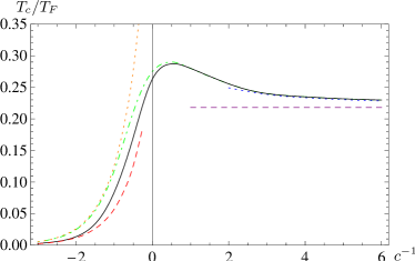
Figure 8: (Color online) Dimensionless critical temperature $T_{\text{c}}/T_{\text{F}}$ as a function of the inverse concentration $c^{-1}=(ak_{\mathrm{F}})^{-1}$. This plot is taken from Ref. FSDW08 . The black solid line includes the effect of particle-hole fluctuations. The result obtained when particle-hole fluctuations are neglected is also shown (dot-dashed line). For comparison, we plot the BCS result without (left dotted line) and with Gorkov’s correction (left dashed). On the BEC side with $c^{-1}>1$ we show the critical temperature for a gas of free bosonic molecules (horizontal dashed line) and a fit to the shift in $T_{\text{c}}$ for interacting bosons, $\Delta T_{\text{c}}\sim c$ (dotted line on the right).

The results from the extended truncation used in FSDW08 are depicted be the solid line in Fig. 8. This result agrees with the prediction by Gorkov and Melik-Barkhudarov in the regime with small negative scattering length (long-dashed line in Fig. 8). By contrast, the simpler truncation described in Sec. II of this paper (dot-dashed line) reproduces the original BCS result (dotted line in Fig. 8). Both our approximations yield the same result for $c^{-1}\gtrsim 0.5$ where the effect of particle-hole fluctuations disappears. This is expected since the chemical potential is negative here, $\mu<0$, and there is no Fermi surface any more. In the BEC limit for very small positive scattering length we find that our result approaches the critical temperature of a free Bose gas

$$\frac{T_{\text{c,BEC}}}{T_{\text{F}}}\approx 0.218.$$ (76)

For $c\to 0_{+}$ this value is approached in the form

$$\frac{T_{\text{c}}-T_{\text{c,BEC}}}{T_{\text{c,BEC}}}=\kappa a_{\text{M}}n_{\text{M}}^{1/3}=\kappa\frac{a_{\text{M}}}{a}\frac{c}{(6\pi^{2})^{1/3}}.$$ (77)

Here, $n_{\text{M}}=n/2$ is the density of molecules and $a_{\text{M}}$ is the scattering length between them. For the ratio $a_{\text{M}}/a$ we use our result $a_{\text{M}}/a=0.718$ obtained from solving the flow equations in vacuum, see sect. IV, since for tightly bound molecules this is the relevant microscopic interaction parameter. For the coefficients determining the shift in $T_{\text{c}}$ compared to the free Bose gas we find $\kappa=1.55$. Given the simplicity of our approach, it is remarkable that our result is near the value $\kappa\simeq 1.3$ found in an effective three dimensional “classical” bosonic theory Baymetal with lattice simulations Arnold:2001mu ; kashurnikov:2001 and with the functional RG using elaborate momentum-dependent truncations Blaizot:2006vr . A direct quantitative comparison is, however, inhibited by the fact that our result may receive contributions from the residual fermionic modes.

At the unitarity point $c^{-1}=0$ we find $T_{\text{c}}/T_{\text{F}}=0.264$ with the approximation used in FSDW08 . The simpler truncation used in Sect II gives $T_{\text{c}}/T_{\text{F}}=0.276$. This should be compared with results from Quantum Monte Carlo simulations: $T_{\text{c}}/T_{\text{F}}=0.15$ MonteCarloBuro ; MonteCarloBulgac and $T_{\text{c}}/T_{\text{F}}=0.245$ MonteCarloAkki . The measurement by L. Luo et al. Luo2007 in an optical trap gives $T_{\text{c}}/T_{\text{F}}=0.29(+0.03/-0.02)$, which is a result based on the study of the specific heat of the system. Further theoretical predictions based on a variety of methods span a whole range of values: $T_{\text{c}}/T_{\text{F}}=0.249$ ($\epsilon$ expansion Nishida:2006br ), $T_{\text{c}}/T_{\text{F}}=0.183$ (Borel-Padé approximation Nishida:2006eu ), $T_{\text{c}}/T_{\text{F}}=0.136$ ($1/N$ expansion Nikolic:2007zz ), $T_{\text{c}}/T_{\text{F}}=0.160$ (2PI techniques Haussmann:2007zz ). This demonstrates that quantitative precision requires a control of the systematic errors in a given approximation scheme. A particular important point concerns the quantitative accuracy in the determination of the density. We will discuss this issue in Sect. VII. If we replace our determination of the density by the “free particle density” we obtain (in the truncation of Sect. II) $T_{\mathrm{c}}/T_{\mathrm{F}}=0.171$.

VI Universal long-range physics close to the phase transition

As the phase transition is approached, one expects to find universal critical behaviour if the temperature is close enough to the critical temperature $T_{\mathrm{c}}$. This feature can be seen directly from the nonperturbative flow equations. The universal behaviour arises from long-range bosonic fluctuations with momenta below $T^{1/2}$ and larger than the inverse correlation length $\xi^{-1}$, and requires $\xi T_{\mathrm{c}}^{1/2}\gg 1$. The temperature acts as an effective infrared cutoff for the influence of the fermion fluctuations on the long-range physics. Correspondingly, for $k/\sqrt{T_{\mathrm{c}}}\ll 1$ the fermion contribution to the flow becomes small and can be neglected. This can be inferred directly from the dependence of the fermionic threshold functions on $k/\sqrt{T}$, as we have discussed after Eq. (21). On the other hand, for $k/\sqrt{T}\ll 1$ the bosonic threshold functions are transmuted to the ones of a classical statistical system for bosons with U(1) symmetry. The infrared flow is governed by a Wilson-Fisher fixed point for the $N=2$ universality class, where $N=2$ corresponds to the two real scalar fields on which global $SO(2)$-transformations act linearly. Following the flow equations to $k\to 0$ leaves no doubt that this universality class governs the critical exponents and amplitude ratios for $T$ sufficiently close to $T_{\mathrm{c}}$. For more elaborate truncations, the non-perturbative flow equations yield precise values for these quantities Berges:2000ew ; Blaizot:2006vr .

It is not our aim here to reproduce the precise universal quantities by an extension of our truncation. We are rather interested in another question: how extended is the temperature range for the universal behavior? Furthermore, we want to compute the non-universal aspects of the phase transition as well. They will depend, of course, on the precise location of the system in the BCS-BEC crossover. As an example, we investigate the temperature dependence of the boson self-interaction $\lambda_{\varphi}$. Close to the critical temperature, $\lambda_{\varphi}$ is known to vanish ($\lambda_{\varphi}^{2}/m_{\varphi}^{2}$ goes to a constant in the symmetric phase). Since also the gap $\Delta$ vanishes for $T\to T_{\mathrm{c}}$, we may take the size of the gap $\Delta(T)$ as a measure of the distance from the critical temperature. In Fig. 9 we plot the ratio $\lambda_{\varphi}(T)/\lambda_{\varphi}(T=0)$ as a function of $\Delta(T)/\Delta(T=0)$.

Figure 9: Boson self-interaction $\lambda_{\varphi}/\lambda_{\varphi}(T=0)$ as a function of the gap parameter $\Delta(T)/\Delta(T=0)$. The corresponding temperature range is $0\leq T\leq T_{\text{c}}$, where $T_{\text{c}}$ corresponds to the origin of the plot. Solid line: BCS regime, $c^{-1}=-2$. Dot-dashed line: crossover regime, $c^{-1}=0$. Dotted line: BEC regime, $c^{-1}=4$.

The plots correspond to the BCS (solid; $c^{-1}=-2$), crossover (dashed dotted; $c^{-1}=0$) and BEC (dotted; $c^{-1}=4$) regimes. In the BEC and unitarity regime, we observe an almost linear increase of $\lambda_{\varphi}$ with $\Delta$ – neglecting effects of a small anomalous dimension, the universal scaling relations indeed suggest $\lambda_{\varphi}/\Delta\to\text{const}$. The linear increase of $\lambda_{\varphi}$ with $\Delta$ extends within a substantial range in temperature. On the BCS side, in contrast, the universal critical region strongly shrinks.

In Fig. 10, we show the slope of $\lambda_{\varphi}/\Delta$ on a logarithmic scale.

Figure 10: Logarithmic slope of $\lambda_{\varphi}$, given by $d\ln\lambda_{\varphi}/d\ln\Delta$, as a function of the gap $\ln[\Delta(T)/\Delta(T=0)]$. Here $T_{\text{c}}$ is approached for large negative values of $\ln\Delta$. Solid line: BCS regime, $c^{-1}=-2$. Dot-dashed line: crossover regime, $c^{-1}=0$. Dotted line: BEC regime, $c^{-1}=4$.

For the BEC and unitarity regime, we can numerically read off the slope, $\lambda_{\varphi}\sim\Delta^{\zeta}$, $\zeta=0.98$. For the unitarity regime ($c^{-1}=0$, dashed dotted line), the universal behavior seems to be reached very quickly, typically already for $\Delta(T)\approx\Delta(0)/2$. This is related to the presence of a strong coupling which induces a fast approach to the infrared fixed point. The universal region is smaller on the BEC side ($c^{-1}=4$, dotted line). In contrast, the approach to the universal fixed point is very slow in the BCS regime ($c^{-1}=-2$, solid line). In consequence, the temperature interval around $T_{\mathrm{c}}$ for which universal behavior occurs is found to be very narrow.

VII Atom density

Since we use the grand canonical formalism, the particle number $n$ is fixed indirectly by the chemical potential $\mu$ which is a parameter of our microscopic model in Eq. (1) similar as the temperature $T$ or the detuning $\nu$. One of the dimensionful parameters can be used to set the scale of the problem, such that actual computations only determine dimensionless combinations of observables as functions of dimensionless combinations of parameters. To compare our results to experiment or other methods one might in principle consider dimensionless quantities that involve $\mu$, for example $T_{\mathrm{c}}/\mu$. For example, with the truncation described in Sect. II, we find at unitarity the ratio $T_{\mathrm{c}}/\mu=0.44$ while the improved truncation in Ref. FSDW08 yields $T_{\mathrm{c}}/\mu=0.39$. This may be compared with the results from Monte-Carlo calculations $T_{\mathrm{c}}/\mu=0.31$ MonteCarloBuro , $T_{\mathrm{c}}/\mu=0.35$ MonteCarloBulgac , from $1/N$-expansion $T_{\mathrm{c}}/\mu=0.232$ Nikolic:2007zz or from 2-PI methods $T_{\mathrm{c}}/\mu=0.41$ Haussmann:2007zz .

However, the rescaling with respect to $\mu$ is not optimal for a comparison to experiments. In contrast to the particle density $n$, the chemical potential $\mu$ is not directly accessible experimentally. Dimensionless ratios that directly involve the particle number such as $T_{\mathrm{c}}/T_{\mathrm{F}}$ with $T_{\mathrm{F}}=(3\pi^{2}n)^{2/3}$ can be measured more directly than $T_{\mathrm{c}}/\mu$.

For strongly interacting particles the dependence $n(\mu)$ is non-trivial to obtain. This is in contrast to weak interactions where $n(\mu)$ can be estimated by the corresponding formula for a non-interacting gas. Part of the uncertainity in the prediction of a dimensionless ratio that involves the density arises therefore from the determination of the function $n(\mu)$. In this paper, we use a flow equation for a scale-dependent generalization of the density,

$$\partial_{k}n_{k}=-\partial_{k}\frac{\partial}{\partial\mu}U_{k},$$ (78)

in order to calculate the density $n=n_{k}|_{k=0}$. The $\mu$ dependence of $U_{k}$ is approximated by an expansion in $\rho$ and $\mu$ as shown in Eq. (22). For the determination of $n$, we need only the terms linear in $\delta\mu$ with $\mu=\mu_{0}+\delta\mu$. Besides the term linear in $\delta\mu$ and $\rho-\rho_{0}$, one might add another term which is quadratic in $\rho-\rho_{0}$. We have checked numerically that the inclusion of such a term has only a very small influence on the quantitative determination of $n$ and neglect it for our numerical results.

In this work, we neglect a possible renormalization of the fermion propagator $G_{\psi}$. This implies also that the dependence on $\mu$ is the same for all cutoff scales $k$. In particular, the effect of fluctuations on the size of the Fermi sphere is not taken into account such that it is of radius $\mu^{1/2}$ an all scales. Beyond our approximation, we expect that the effect of a $k$-dependent Fermi sphere changes somewhat the dependence of the density $n$ on the chemical potential $\mu$.

To illustrate the importance of the density determination, we compare our result for $T_{\mathrm{c}}/T_{\mathrm{F}}$ with a calculation where a much simpler (and naive) method is used to estimate the density. It is motivated physically by assuming that we have simply coexisting pointlike atoms and dimers, which are coupled via a common chemical potential Diehl:2005ae – in this picture, strong correlation effects are completely omitted for the density determination, and we can get an impression of the sensitivity of our results with respect to such correlation effects. At the critical temperature the superfluid and condensate densities vanish and no occupation number density for a single momentum mode is expected to be of the order $n$. In addition, the energy gap for the bosons just vanishes, $m_{\varphi}^{2}=0$. Neglecting the effect of interactions, one could use a naive estimate for the density at $T=T_{\mathrm{c}}$,

$$n_{\text{naive}}=\int\frac{d^{3}p}{(2\pi)^{3}}\left\{\frac{2}{e^{(\vec{p}^{2}-\mu)/T_{\mathrm{c}}}+1}+\frac{2}{e^{\vec{p}^{2}/(2T_{\mathrm{c}})}-1}\right\}.$$ (79)

The first term gives the contribution of the fermions where the factor $2$ counts the spin-states. As stated above, the second contribution comes from the bosons and the factor $2$ reflects now that every boson consists of two fermions. Our flow equation method yields a result for $n$ that is roughly a factor $1/2$ smaller than $n_{\text{naive}}$. Correspondingly, the ratio $T_{\mathrm{c}}/T_{\mathrm{F}}$ is larger. For a comparison of both methods, we plot $T_{\mathrm{c}}/T_{\mathrm{F}}$ as a function of $c^{-1}$ in Fig. 11. At the unitarity point $c^{-1}=0$, the formula in Eq. (79) leads to $T_{\mathrm{c}}/T_{\mathrm{F}}=0.171$.

As a side remark, we note that the approximation made to obtain Eq. (79) becomes valid for extremely narrow resonances with vanishing Yukawa interaction $h_{\varphi}\to 0$ Diehl:2005ae . Of course, the strongly interacting problem we are interested in here is the opposite limit of broad resonances $h_{\varphi}\to\infty$ – here, we only try to estimate the uncertainty emerging from the neglect of correlation effects on the density.

Figure 11: (Color online) Dimensionless critical temperature $T_{\text{c}}/T_{\text{F}}$ as a function of the inverse concentration $c^{-1}=(ak_{\mathrm{F}})^{-1}$. We show the result obtained in the truncation descibed in Sec. II with the flow equation for the density (solid line). In addition we show the result obtained using the simpler (naive) estimate for the density in Eq. (79) (long dashed line). The dotted line gives the critical temperature of a free BEC while the short-dashed line is the expected correction for an interacting Bose gas in Eq. (77), with the Monte-Carlo result $\kappa=1.3$ and with $a_{M}/a=0.6$ Petrov04 .

At the phase transition we have two independent (dimensionless) ratios $T_{\mathrm{c}}/T_{\mathrm{F}}$ and $\mu/T_{\mathrm{F}}$. For the unitarity limit, $c^{-1}=0$ we display these ratios for different approximations and compare them to Monte-Carlo results in table 1. The lack of agreement may indicate that the truncation should be improved further, and we discuss various directions in the conclusions. Another insufficiency of the present truncation becomes visible in the behaviour of the superfluid density for $T\to 0$, as shown in Fig. 12. The ratio $n_{\mathrm{S}}/n$ should remain smaller than one, which is not obeyed by our current truncation on the BCS side. At zero temperature Galilean invariance implies $n=n_{S}$ throughout the whole BCS-BEC crossover. We expect that the problem can be solved by including the $\rho$ dependence of the wavefunction renormalization $A_{\varphi}$ where the dependence on $\rho$ was neglected in our truncation.

	$\,\,\,T_{\mathrm{c}}/T_{\mathrm{F}}\,\,\,$	$\,\,\,\mu/T_{\mathrm{F}}\,\,\,$	$\,\,\,T_{\mathrm{c}}/\mu\,\,\,$
Truncation Sect. II	0.276	0.63	0.44
Truncation including	0.245	0.63	0.39
particle-hole fluc. FSDW08
Density according	0.171	0.39	0.44
to Eq. (79)
Monte-Carlo MonteCarloBuro	0.152(7)	0.493(17)	0.31
Monte-Carlo MonteCarloBulgac	0.15(1)	0.43(1)	0.35

Table 1: Critical temperature $T_{\mathrm{c}}$, critical density $n_{c}$ (expressed through the Fermi temperature $T_{\mathrm{F}}=(3\pi^{2}n_{c})^{2/3}$), and chemical potential $\mu$ in the “unitarity limit” of infinite scattering length $c^{-1}=0$.

Figure 12: Superfluid fraction $n_{\mathrm{S}}/n=2\rho_{0}/n$ as a function of temperature $T/T_{\mathrm{F}}$. We show the curves obtained on the BCS side with $c^{-1}=-1$ (dashed line), in the unitarity regime with $c^{-1}=0$ (solid line) and on the BEC side with $c^{-1}=1$ (dashed-dotted line) and $c^{-1}=2$ (dotted line). While the superfluid fraction approaches $1$ for small temperatures on the BEC side, this is not the case on the BSC side and in the unitarity regime. This feature is an artefact of our present truncation.

VIII Conclusion

In this paper, we have given a rather detailed account of the use of the flowing action for ultracold fermionic atoms. Our method allows for a unified approach for all temperatures and densities – including the vacuum for $T=n=0$ – as well as arbitrary scattering length. The overall picture of the phase transition to the low-temperature superfluid phase and the BCS-BEC crossover as a function of the scattering length or concentration $c=ak_{\text{F}}$ is rather satisfactory. In particular, the dependence of the critical temperature $T_{\mathrm{c}}$ on the scattering length yields the effects of interactions between composite molecules on the BEC side, as well as the correct behaviour on the BCS side including the effect of particle-hole fluctuations. The largest uncertainties occur in the “unitarity limit” $c^{-1}=0$ of very large scattering length. In this region in parameter space, the fluctuations are strongest and possible deviations of the effective action from our rather simple truncation are expected to be largest. As far as the critical temperature for $c^{-1}=0$ is concerned, the comparison with the Monte-Carlo results in table 1 may give an idea of the uncertainties.

The phase diagram can be computed from the dependence of the effective boson potential $U(\varphi)$ on the temperature and density or $T$ and $\mu$. The exact flow equation (II.2) for the flowing potential $U_{k}(\varphi)$ involves the exact propagators of fermions and composite bosons in the presence of a constant background field $\varphi$ – the condensate corresponds to the value of $\varphi_{0}$ for which the minimum of $U(\varphi)$ occurs. The present truncation (Eqs. (8), (17)) of the propagators remains rather crude and we expect a considerable quantitative improvement for truncations with a more detailed resolution of the dependence of the propagators on momentum and frequency, as well as their dependence on $\varphi$. On the other hand, increased precision also needs an increased accuracy in the parameters used in a given truncation of the propagators. They are determined by exact flow equations for the inverse propagators which involve, in turn, the cubic and quartic vertices. In this respect the accuracy may be enhanced by a more complicated truncation of the momentum and frequency dependence of the effective four-fermion interaction, beyond the molecule-exchange channel on which we have concentrated in this paper. In this respect, methods of rebosonization which closely keep track of the relation between the composite field $\varphi$ and its fermionic constituents FWCompositeoperators could lead to an impoved treatment of particle-hole fluctuations for large scattering length.

The effort of improving the truncation leads not only to an increased accuracy of the phase diagram. Simultaneously, many detailed features of the propagators become available. We have demonstrated this briefly by our computation of the correlation length. Furthermore, many thermodynamic quantities can be computed from the dependence of $U$ on $T$ and $\mu$, as specific heat, compressibility, or sound velocities. This has been demonstrated for bosonic atoms in FWThermod and the same methods could be taken over to the BEC-BCS crossover system. Further generalizations concern systems with three or more species of fermions FSMW or unequal abundances of different fermion species Gubbels:2008zz ; Ku:2008vk . We hope that the generality and flexibility of our treatment will lead to a unified treatment of many interesting features encountered in these systems, and simultaneously permit quantitative accuracy of the theoretical estimates, as needed for precision measurements.

Appendix A Units

In this work, our units are chosen such that $\hbar=k_{\text{B}}=2M=1$, where $M$ is the mass of the fermionic atoms. Setting $\hbar=1$ implies that space coordinates and inverse momenta are measured in terms of the same dimensionful scale. The choice $k_{\text{B}}=1$ similarly establishes an equivalent measurement of energy and temperature in terms of the same scale. Setting $2M=1$ finally relates the measurement scales of energy and temperature on the one hand to squared momenta or inverse squared coordinates on the other hand. (The meaning of the latter choice is similar to setting the velocity of light $c=1$ in relativistic theories). Only one unit remains free, say the length $l$, with dimensions $[t]=l^{2}$, $[\vec{q}]=l^{-1}$, $[T]=l^{-2}$, $[\mu]=l^{-2}$, and $[n]=l^{-3}$.

In practice, these units are obtained by rescaling the coordinates $x/\hbar\to x$ for $\hbar=1$, the temperature $k_{\text{B}}T\to T$ for $k_{\text{B}}=1$, and the time $\tau/2M\to\tau$ for $2M=1$. The last step goes along with rescaling also all interaction terms of the action: $2MS_{\text{int}}\to S_{\text{int}}$. All dimensionful quantities are then measured in terms of only one dimensionful scale which we set in terms of the density $n$ of the system or, equivalently, in terms of the Fermi momentum

$$k_{\text{F}}=(3\pi^{2}n)^{1/3}.$$ (80)

Typical values of the Fermi momentum occurring in trapped Fermi-gas experiments are of the order $k_{\text{F}}\sim\mathcal{O}(1\dots 10\mathrm{eV}/c)$ in units of electron Volt/$c$ (The light velocity $c$ occurs here to convert the energy unit eV into a momentum). With our choice of units, $k_{\text{F}}=1$eV/$c$ corresponds to a density $n\simeq 4.4\times 10^{12}\mathrm{cm}^{-3}$ for which we have used that 1eV/$c\simeq 5.07\times 10^{6}\mathrm{m}^{-1}$ in our units with $\hbar=1$. A typical length scale such as the Bohr radius $a_{\text{B}}=5.29177\times 10^{-11}\mathrm{m}$ then reads in inverse momentum units $a_{\text{B}}=2.6817\times 10^{-4}(\mathrm{eV}/c)^{-1}$.

Energy- or temperature-like quantities can most conveniently be measured in terms of the Fermi energy or Fermi temperature which are equivalent in our units,

$$\epsilon_{\text{F}}\equiv T_{\text{F}}=\frac{k_{\text{F}}^{2}}{2M}\equiv k_{\text{F}}^{2}.$$ (81)

As $1\equiv 2M=2\frac{M}{\mathrm{eV}/c^{2}}\,\mathrm{eV}/c^{2}$, fixing the atom mass $M$ in units of eV/$c^{2}$ (e.g., $M_{{}^{6}\mathrm{Li}}\simeq 5.6\times 10^{9}\mathrm{eV}/c^{2}$ for Lithium-6) corresponds to expressing the velocity of light $c$ in units of $\sqrt{\mathrm{eV}}$. This establishes eV units for our energy-like quantities such as the Fermi energy.

As shown in the main text, the scattering length $a$ remains as the only physical parameter of the interacting Fermi gas in the broad-resonance limit. Together with the temperature, the relevant dimensionless quantities characterizing the phase diagram are

$$c^{-1}=(ak_{\text{F}})^{-1},\quad\frac{T}{T_{\text{F}}}=\frac{T}{k_{\text{F}}^{2}},$$ (82)

where $c$ (not to be confused with the velocity of light here) can be viewed as a concentration parameter, as it measures the inverse scattering length in units of the interparticle spacing $\sim k_{\text{F}}^{-1}$.

We use our result for the critical temperature at unitarity, $T_{\text{c}}/T_{\text{F}}\simeq 0.276$ at $ak_{\text{F}}=0$, to illustrate how to convert our results into standard laboratory units, using Lithium-6 as an example. First, we assume an atom density of $n=10^{13}\mathrm{cm}^{-3}$ which implies $k_{\text{F}}\simeq 1.3\mathrm{eV}/c$. The resulting critical temperature reads $T_{\text{c}}\simeq 0.276T_{\text{F}}\simeq 0.477(\mathrm{eV}/c)^{2}$. In our units, where the Lithium-6 mass obeys $2M=1$, the velocity of light can be expressed as $c=\sqrt{2\frac{M}{\mathrm{eV}/c^{2}}\mathrm{eV}}\simeq 1.06\times 10^{5}\sqrt{\mathrm{eV}}$. Inserting this into the critical temperature yields $T_{\text{c}}\simeq 4.26\times 10^{-11}\mathrm{eV}\simeq 0.49\mu\mathrm{K}$.

Appendix B Symmetries

Symmetries of the microscopic action $S$ are also symmetries of the effective action $\Gamma$, provided the functional measure does not give rise to an anomaly and that the infrared cutoff respects the symmetry. The symmetries of $\Gamma$ severely restrict its possible form. They are therefore helpful in devising useful truncations. All truncations should be consistent with the symmetries.

In our case we have first the symmetries of translations in space and time and the rotation symmetry in space. Further, a continuous U(1) symetry reflects the conserved number of atoms.

$$\psi_{1}\rightarrow e^{i\alpha}\psi_{1}, \psi_{1}^{\ast}\rightarrow e^{-i\alpha}\psi_{1}^{\ast}$$

$$\psi_{2}\rightarrow e^{i\alpha}\psi_{2}, \psi_{2}^{\ast}\rightarrow e^{-i\alpha}\psi_{2}^{\ast}$$

$$\varphi\rightarrow e^{2i\alpha}\varphi, \varphi^{\ast}\rightarrow e^{-2i\alpha}\varphi^{\ast}.$$ (83)

This symmetry is conserved by the cutoff and easily realized in truncations by including in $\Gamma$ only terms with total atom number zero. (Here $\psi$ and $\varphi$ have atom number one and two, and $\psi^{*}$, $\varphi^{*}$ the corresponding negative numbers.) The action (1) also shows an SU(2)-symmetry of “spin rotations” between the two fermion components. This is again easily implemented. Further discrete symmetries are parity reflections ($\psi(\tau,\vec{x})\to\psi(\tau,-\vec{x})$, $\varphi(\tau,\vec{x})\to\varphi(\tau,-\vec{x})$) as well as euclidean time reflection

$$\psi_{1}(\tau,\vec{x})\rightarrow \psi_{1}^{\ast}(-\tau,\vec{x}),\quad \psi_{1}^{\ast}(\tau,\vec{x})\rightarrow-\psi_{1}(-\tau,\vec{x}),$$

$$\psi_{2}(\tau,\vec{x})\rightarrow -\psi_{2}^{\ast}(-\tau,\vec{x}),\quad \psi_{2}^{\ast}(t,\vec{x})\rightarrow\psi_{2}(-\tau,\vec{x}),$$

$$\varphi(\tau,\vec{x})\rightarrow \varphi^{\ast}(-\tau,\vec{x}),\quad \varphi^{\ast}(\tau,\vec{x})\rightarrow\varphi(-\tau,\vec{x}).$$ (84)

We note that $\psi_{\alpha}$ and $\psi_{\alpha}^{\ast}$ are separate Grassmann variables for which the structure of complex conjugation is not defined a priori. The transformation (84) is actually not compatible with the usual complex structure. (The action (1) is also invariant under $\varphi(\tau,\vec{x})\leftrightarrow\varphi^{*}(-\tau,\vec{x})$, $\psi_{\alpha}(\tau,\vec{x})\leftrightarrow\psi_{\alpha}(-\tau,\vec{x})$ if all Grassmann variables are completely reordered.) Time reflection symmetry does not forbid terms with an even number of $\tau$-derivatives.

For zero temperature no rest frame is singled out a priori and we expect invariance under Galilei-transformations. The implications of Galilean invariance can be understood best if we perform an analytic continuation from euclidean time to real time $\tau=it$. The microscopic action (1) becomes then

$$S[\varphi,\psi]=i\int_{-\infty}^{\infty}dt\int d^{3}x\Bigl{(}\psi^{\dagger}\left(-i\partial_{t}-\Delta-\mu\right)\psi$$

$$\hskip 34.14322pt+\varphi^{\ast}\left(-i\partial_{t}-\frac{1}{2}\Delta+\nu-2\mu\right)\varphi$$

$$\hskip 34.14322pt-h_{\varphi}\left(\varphi^{\ast}\psi^{T}\epsilon\psi-\varphi\psi^{\dagger}\epsilon\psi^{\ast}\right)\Bigr{)}\,.$$ (85)

Galilean boost transformations (with a boost velocity $2\vec{q}$) act on the fields as

$$\psi(t,\vec{x})\rightarrow\psi^{\prime}(t,\vec{x}) = e^{-i(\vec{q}^{2}t-\vec{q}\vec{x})}\psi(t,\vec{x}-2\vec{q}t)$$

$$\varphi(t,\vec{x})\rightarrow\varphi^{\prime}(t,\vec{x}) = e^{-2i(\vec{q}^{2}t-\vec{q}\vec{x})}\varphi(t,\vec{x}-2\vec{q}t).$$ (86)

While the invariance of the Yukawa term under this transformation is obvious, its realization for the kinetic term is more involved. Performing the transformation explicitly one finds

$$\psi^{\dagger}\Delta\psi \rightarrow \psi^{\dagger}\Delta\psi-\vec{q}^{2}\psi^{\dagger}\psi+2i\vec{q}\psi^{\dagger}\vec{\nabla}\psi$$

$$\varphi^{\dagger}\Delta\varphi \rightarrow \varphi^{\dagger}\Delta\varphi-4\vec{q}^{2}\psi^{\dagger}\varphi+4i\vec{q}\varphi^{\dagger}\vec{\nabla}\varphi$$

$$\psi^{\dagger}i\partial_{t}\psi \rightarrow \psi^{\dagger}i\partial_{t}\psi+\vec{q}^{2}\psi^{\dagger}\psi-2i\vec{q}\psi^{\dagger}\vec{\nabla}\psi$$

$$\varphi^{\dagger}i\partial_{t}\varphi \rightarrow \varphi^{\dagger}i\partial_{t}\varphi+2\vec{q}^{2}\varphi^{\dagger}\varphi-2i\vec{q}\varphi^{\dagger}\vec{\nabla}\varphi,$$ (87)

such that indeed the combinations

$$-i\partial_{t}-\Delta$$ (88)

for the fermions and

$$-i\partial_{t}-\frac{\Delta}{2}$$ (89)

for the bosons lead to this invariance. The conserved Noether charge of Galilean symmetry is the center of mass momentum.

In the case of a bosonic condensate $\varphi(\vec{x},t)=\varphi_{0}$ the Galilean symmetry is spontaneously broken. Now the condensate determines the rest frame. The spontaneous symmetry breaking of Galilean symmetry comes in pair with spontaneous symmetry breaking of the U(1) symmetry associated to atom number. It can be associated with superfluidity. We stress that for $T>0$ Galilean symmetry is explicitly broken since the heat bath singles out a rest frame. For low temperatures truncations consistent with Galilean transformations (and therefore always containing the combinations (88) and (89) remain useful, however, since symmetry breaking terms vanish for $T\to 0$.

Finally, we observe another useful invariance of the action for $T=0$. It arises if we consider $\mu$ as a source term for the fermion and boson bilinears and consider transformations that also change $\mu$. (These type of invariances are not symmetries of the action in the standard sense, since “parameters” of the action are changed by the transformation.) Let us extend Eq. (85) to a $t$-dependent source $\mu(t)$. There is now a semilocal $U(1)$ invariance of the form

$$\psi\rightarrow e^{i\alpha(t)}\psi,\quad\psi^{\dagger}\rightarrow e^{-i\alpha(t)}\psi^{\dagger}$$

$$\varphi\rightarrow e^{2i\alpha(t)}\varphi,\quad\varphi^{\ast}\rightarrow e^{-2i\alpha(t)}\varphi^{\ast}$$

$$\mu\rightarrow\mu+\partial_{t}\alpha.$$ (90)

This holds, since the combinations $(-i\partial_{t}-\mu)$ and $(-i\partial_{t}-2\mu)$ act as covariant derivatives for the fermions and bosons, respectively.

Combining semi-local $U(1)$ symmetry and Galilean symmetry at $T=0$ we find, that the derivative operators and the chemical potential are combined to the operator

$$D_{\psi}=(-i\partial_{t}-\Delta-\mu)$$ (91)

for the fermions and

$$D_{\varphi}=(-i\partial_{t}-\frac{\Delta}{2}-2\mu)$$ (92)

for the bosons. In addition to powers of this operator, only spatial derivative of terms that are invariant under $U(1)$ transformations like e.g. $\rho\Delta\rho$ with $\rho=\varphi^{\ast}\varphi$ may appear. The above symmetry transformations act linearly on the fields and so also the effective action $\Gamma$ is invariant. Also there, only powers of the operators $D_{\psi}$ and $D_{\varphi}$ may act on the fields $\psi$ and $\varphi$.

In the presence of spontaneous symmetry breaking by a nonvanishing order parameter $\rho=\varphi^{\ast}\varphi>0$ the possibilities for combining space and time derivatives get more complex. Effectively, terms quadratic in $\partial_{t}$ need not be matched by terms quadratic in $\Delta$ or $\mu$. For a more detailed discussion see FloerchingerWetterich . Let us finally mention, that there is an additional conformal invariance at the unitary point in the crossover where the fermion scattering length diverges $c=ak_{\text{F}}=\infty$ Son:2005rv . The only length scale is then set by the chemical potential $\mu$ or by the particle number density $n$. This gives further constraints to the effective action at that point in the phase diagram.

Appendix C Cutoff functions

The computations in the present work are done with regulators which are optimised w.r.t. the derivative expansion, see e.g. Litim:2000ci ; Litim:2001up ; Pawlowski:2005xe . Such a choice stabilises the truncation and minimizes the systematical error for the computed observables. For the scalar field we choose the Litim regulator Litim:2000ci

$$R_{k}^{(\varphi)}(q^{2}) = A_{\varphi}k^{2}r_{k\varphi}(y)\,,\quad y=\frac{q^{2}}{2k^{2}}\,,$$

$$r_{k\varphi}(y) = (1-y)\theta(1-y)\,.$$ (93)

Combining the $\vec{q}^{2}$-dependent term in the inverse propagator $G_{\varphi}^{-1}$ with the cutoff term one finds for $P_{\varphi}=\vec{q}^{2}/2+R_{k}^{(\varphi)}/A_{\varphi}$ the simple behavior $P_{\varphi}=\vec{q}^{2}/2$ for $\vec{q}^{2}>2k^{2}$, $P_{\varphi}=k^{2}$ for $\vec{q}^{2}<2k^{2}$. In other words, our regulator leaves the propagation of modes with spatial momenta bigger than the cut-off scale, $q^{2}\geq 2k^{2}$, unchanged. For modes with spatial momenta smaller than the cut-off scale, $q^{2}<2k^{2}$, it effectively introduces an infrared mass term $k^{2}$.

For the fermionic field we choose an analogue of the scalar regulator (93). Here, however, the propagation of modes close to the Fermi surface is suppressed,

$$R_{k}^{(\psi)}(q^{2}) = k^{2}r_{k\psi}(z)\,,$$

$$r_{k\psi}(z) = (\text{sign}(z)-z)\theta(1-|z|)\,,$$ (94)

where

$$z=(q^{2}-\mu)/k^{2}.$$ (95)

This regulator leaves the propagation of modes with spatial momenta farther away from the Fermi surface than the cut-off scale, $q^{2}-\mu\geq k^{2}$, unchanged but leads to a flat (inverse) propagator $k^{2}$ for modes with spatial momenta closer to the Fermi surface than the cut-off scale $q^{2}-\mu<k^{2}$. This effectively introduces an infrared mass term proportional to $k^{2}$. In summary this takes into account the fact that fermionic fluctuations have to be cut-off relative to the Fermi surface, and hence introduces to leading order the same cut-off scales for the fermionic and bosonic fluctuations. The fermionic regulator in the presence of a Fermi surface is displayed in Fig. 13.

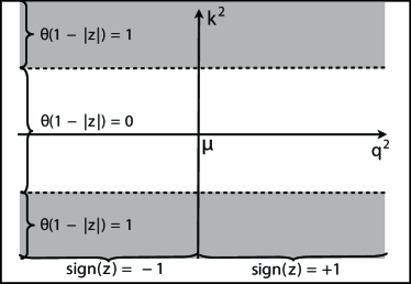
Figure 13: The fermionic regulator in the presence of a Fermi surface $\mu>0$.

Appendix D Flow of the effective potential

In this App. we derive the flow equation for the effective potential $U(\rho,\mu)$. We start from the exact flow equation for the average action (or flowing action) Wetterich:1992yh

$$\partial_{k}\Gamma_{k}=\frac{1}{2}\text{STr}(\Gamma_{k}^{(2)}+R_{k})^{-1}\partial_{k}R_{k}.$$ (96)

This is evaluated for a bosonic field $\bar{\varphi}$ that is constant in space and in (Matsubara-) time, $\bar{\varphi}(\vec{x},\tau)=\bar{\varphi}$. (The expectation value of the fermionic field $\psi$ vanishes – for vanishing fermion source – due to its Grassmann property.) Using the truncation in Eq. (II.3) we find the flow equation for the potential

$$\partial_{k}U_{k}{\big{|}}_{\bar{\rho}} = \frac{1}{2}\int\limits_{q_{0},\vec{q}}{\bigg{\{}}\left[(G_{k\varphi})_{11}+(G_{k\varphi})_{22}\right]A_{\varphi}^{-1}\partial_{k}\left(A_{\varphi}k^{2}r_{k\varphi}\right)$$ (97)

$$- \left[(G_{k\psi})_{13}+(G_{k\psi})_{24}-(G_{k\psi})_{31}-(G_{k\psi})_{42}\right]$$

$$\times\partial_{k}\left(k^{2}r_{k\psi}\right){\bigg{\}}},$$

which is evaluated for fixed $\bar{\rho}=\bar{\varphi}^{*}\bar{\varphi}$. The dimensionless function $r_{k\varphi}$ depends on $y=\vec{q}^{2}/(2k^{2})$ while $r_{k\psi}$ depends on $z=(\vec{q}^{2}-\mu_{0})/k^{2}$. The regularized propagators $G_{k\varphi}$ and $G_{k\psi}$ that appear in Eq. (97) are modified from Eqs. (11) (17) by the presence of the ultraviolet regulator

$$G_{k\varphi}^{-1} = G_{\varphi}^{-1}+\begin{pmatrix}k^{2}r_{k\varphi}&&0\\ 0&&k^{2}r_{k\varphi}\end{pmatrix}$$

$$G_{k\psi}^{-1} = G_{\psi}^{-1}+\begin{pmatrix}0&&-k^{2}r_{k\psi}\\ k^{2}r_{k\psi}&&0\end{pmatrix}.$$ (98)

We can now perform the summation over the Matsubara frequencies $q_{0}=2\pi Tn$ for the bosons and $q_{0}=2\pi T(n+1/2)$ for the fermions. The integration over $\vec{q}$ is performed quite generally in $d$ spatial dimensions. The result can be expressed in terms of the dimensionless variables

$$w_{1}=\frac{U_{k}^{\prime}}{k^{2}},\quad w_{2}=\frac{U_{k}^{\prime}+2\rho U_{k}^{\prime\prime}}{k^{2}},\quad w_{3}=\frac{h_{\varphi}^{2}\rho}{k^{4}},$$

$$\tilde{\mu}=\frac{\mu_{0}}{k^{2}},\quad\Delta\tilde{\mu}=\frac{\mu-\mu_{0}}{k^{2}},\quad\tilde{T}=\frac{T}{k^{2}},\quad S_{\varphi}=\frac{Z_{\varphi}}{A_{\varphi}},$$ (99)

and the anomalous dimension

$$\eta_{A_{\varphi}}=-\frac{k\partial_{k}A_{\varphi}}{A_{\varphi}}.$$ (100)

A term involving the anomalous dimension appears if we evaluate the flow for fixed $\rho=A_{\varphi}\bar{\rho}$ instead of fixed $\bar{\rho}$. The flow of the effective potential reads now

$$k\partial_{k}U_{k} = \eta_{A_{\varphi}}\,\rho\,U_{k}^{\prime}+8\sqrt{2}\frac{k^{d+2}v_{d}}{d\,S_{\varphi}}\left(1-\frac{2}{d+2}\eta_{A_{\varphi}}\right)s_{\text{B}}^{(0)}$$ (101)

$$-\,8\frac{k^{d+2}v_{d}}{d}\,l(\tilde{\mu})\,s_{\text{F}}^{(0)}.$$

Here, the coefficient $v_{d}$ is proportional to the surface of the $d$-dimensional unit sphere, which is $(2\pi)^{d}4v_{d}$, with $v_{d}^{-1}=2^{d+1}\pi^{d/2}\Gamma(d/2)$. In particular one has $v_{3}=1/(8\pi^{2})$.

The threshold functions $s_{\text{B}}^{(0)}=s_{\text{B}}^{(0)}(w_{1},w_{2},\tilde{T},S_{\varphi},\eta_{A_{\varphi}})$ and $s_{\text{F}}^{(0)}=s_{\text{F}}^{(0)}(w_{3},\tilde{\mu},\Delta\tilde{\mu},\tilde{T})$ as well as the function $l(\tilde{\mu})$ used in Eq. (101) depend on the choice of the infrared regulator functions $r_{k\varphi}$ and $r_{k\psi}$. They describe the decoupling of modes when the effective “masses” $w_{j}$ or $-\tilde{\mu}$ get large. The threshold functions for the bosonic fluctuations reads

$$\left(1-\frac{2\,\eta_{A_{\varphi}}}{d+2}\right)s_{\text{B}}^{(0)}=d\int\limits_{0}^{\infty}dy\,y^{\frac{d}{2}-1}\left(r_{k\varphi}-yr_{k\varphi}^{\prime}-\eta_{A_{\varphi}}r_{k\varphi}\right)$$

$$\times\frac{\frac{1}{2}(w_{1}+w_{2})+y+r_{k\varphi}}{\sqrt{w_{1}+y+r_{k\varphi}}\sqrt{w_{2}+y+r_{k\varphi}}}$$

$$\times\left[\frac{1}{2}+N_{\text{B}}(\sqrt{w_{1}+y+r_{r\varphi}}\sqrt{w_{2}+y+r_{k\varphi}}/S_{\varphi})\right],$$

and involves the Bose function

$$N_{\text{B}}(\epsilon)=\frac{1}{e^{\epsilon/\tilde{T}}-1}.$$ (103)

and the optimized cutoff function Litim:2000ci

$$r_{k\varphi}(y)=(1-y)\theta(1-y).$$ (104)

We normalize the threshold function such that $s_{\text{B}}^{(0)}=1$ for $w_{1}=w_{2}=\tilde{T}=0$. For our cutoff one finds the particular simple expression

$$s_{\text{B}}^{(0)} = \left[\sqrt{\frac{1+w_{1}}{1+w_{2}}}+\sqrt{\frac{1+w_{2}}{1+w_{1}}}\right]$$ (105)

$$\times\left[\frac{1}{2}+N_{\text{B}}(\sqrt{1+w_{1}}\sqrt{1+w_{2}}/S_{\varphi})\right].$$

The threshold function for the fermionic fluctuations is obtained similar. For a generic cutoff that addresses the spatial momentum, it reads

$$l(\tilde{\mu})s_{\text{F}}^{(0)}=d\int_{-\tilde{\mu}}^{\infty}dz\,(z+\tilde{\mu})^{\frac{d}{2}-1}\left(r_{k\psi}-zr_{k\psi}^{\prime}\right)$$

$$\times\frac{(z+r_{k\psi}-\Delta\tilde{\mu})}{\sqrt{w_{3}+(z+r_{k\psi}-\Delta\tilde{\mu})^{2}}}$$

$$\times\left[\frac{1}{2}-\,N_{\text{F}}\left(\sqrt{w_{3}+(z+r_{k\psi}-\Delta\tilde{\mu})^{2}}\right)\right].$$ (106)

Here we employ the Fermi function

$$N_{\text{F}}(\epsilon)=\frac{1}{e^{\epsilon/\tilde{T}}+1}.$$ (107)

Note that for a generic cutoff the right hand side of equation (106) does not necessarily factorize. In that case one might work with a threshold function $s_{\text{F}}^{(0)}$ that also depends on $\tilde{\mu}$. For our cutoff

$$r_{k\psi}=(\text{sign}(z)-z)\theta(1-|z|).$$ (108)

one has $s_{\text{F}}^{(0)}=1$ for $w_{3}=\tilde{\mu}=\Delta\tilde{\mu}=0$. For $\mu=\mu_{0}$ and therefore $\Delta\tilde{\mu}=0$ the threshold function assumes the simple form

$$s_{\text{F}}^{(0)}=\frac{2}{\sqrt{1+w_{3}}}\left[\frac{1}{2}-\,N_{\text{F}}\left(\sqrt{1+w_{3}}\right)\right]$$

while

$$l(\tilde{\mu})=\theta(\tilde{\mu}+1)(\tilde{\mu}+1)^{d/2}-\theta(\tilde{\mu}-1)(\tilde{\mu}-1)^{d/2}.$$ (109)

In the limit $\tilde{T}=T/k^{2}\to 0$ the thermal contributions to the flow of $U_{k}$ vanish, $N_{\text{B}}=N_{\text{F}}=0$.

Taking a derivative with respect to $\rho$ on both sides of Eq. (101) we obtain

$$k\partial_{k}U_{k}^{\prime} = \eta_{A_{\varphi}}(U_{k}^{\prime}+\rho U_{k}^{\prime\prime})-8\sqrt{2}\frac{k^{d}v_{d}}{dS_{\varphi}}\left(1-\frac{2}{d+2}\eta_{A_{\varphi}}\right)$$ (110)

$$\times\left[U_{k}^{\prime\prime}s_{\text{B}}^{(1,0)}+(3U_{k}^{\prime\prime}+2\rho U_{k}^{(3)})s_{\text{B}}^{(0,1)}\right]$$

$$+8\frac{k^{d-2}v_{d}}{d}h_{\varphi}^{2}\,l(\tilde{\mu})\,s_{\text{F}}^{(1)}.$$

Here we introduce the derivatives of the threshold functions

$$s_{\text{B}}^{(1,0)} = -\frac{\partial}{\partial w_{1}}s_{\text{B}}^{(0)}$$

$$s_{\text{B}}^{(0,1)} = -\frac{\partial}{\partial w_{2}}s_{\text{B}}^{(0)}$$

$$s_{\text{F}}^{(1)} = -\frac{\partial}{\partial w_{3}}s_{\text{F}}^{(0)}.$$

We may divide these into contributions from quantum and thermal fluctuations

$$s_{\text{B}}^{(1,0)} = (w_{2}-w_{1})s_{\text{B,Q}}^{(1,0)}+s_{\text{B},T}^{(1,0)},$$

$$s_{\text{B}}^{(0,1)} = (w_{2}-w_{1})s_{\text{B,Q}}^{(0,1)}+s_{\text{B},T}^{(0,1)},$$

$$s_{\text{F}}^{(1)} = s_{\text{F,Q}}^{(1)}+s_{\text{F},T}^{(1)}.$$ (112)

For $\tilde{T}\to 0$ the thermal contribution vanishes $s_{\text{B},T}^{(0,1)}=s_{\text{B},T}^{(1,0)}=s_{\text{F},T}^{(1)}=0$. We extracted a factor $(w_{2}-w_{1})$ from the threshold functions $s_{\text{B,Q}}^{(1,0)}$ and $s_{\text{B,Q}}^{(0,1)}$ to make explicit that these contributions vanish for $w_{1}=w_{2}$, which holds for $\rho=0$.

For our choice of the regulator functions $r_{k,\psi}$ and $r_{k\varphi}$ we find the explicit expressions

$$s_{\text{B,Q}}^{(1,0)} = \frac{1}{4(1+w_{1})^{3/2}(1+w_{2})^{1/2}},$$

$$s_{\text{B,Q}}^{(0,1)} = -\frac{1}{4(1+w_{1})^{1/2}(1+w_{2})^{3/2}},$$

$$s_{\text{F,Q}}^{(1)} = \frac{1}{2(1+w_{3})^{3/2}}.$$

For $\tilde{T}>0$ the thermal fluctuations lead to the additional contributions from the bosons

$$s_{\text{B},T}^{(1,0)} = 2(w_{2}-w_{1})\,s_{\text{B,Q}}^{(1,0)}\,N_{\text{B}}\left(\sqrt{(1+w_{1})(1+w_{2})}/S_{\varphi}\right)$$

$$+ s_{\text{B,Q}}^{(0)}\frac{\sqrt{1+w_{2}}}{\sqrt{1+w_{1}}S_{\varphi}}\,N_{\text{B}}^{\prime}\left(\sqrt{(1+w_{1})(1+w_{2})}/S_{\varphi}\right),$$

$$s_{\text{B},T}^{(0,1)} = 2(w_{2}-w_{1})\,s_{\text{B,Q}}^{(1,0)}\,N_{\text{B}}\left(\sqrt{(1+w_{1})(1+w_{2})}/S_{\varphi}\right)$$

$$+ s_{\text{B,Q}}^{(0)}\frac{\sqrt{1+w_{1}}}{\sqrt{1+w_{2}}S_{\varphi}}\,N_{\text{B}}^{\prime}\left(\sqrt{(1+w_{1})(1+w_{2})}/S_{\varphi}\right).$$

Here, we use the derivative of the Bose function

$$N_{\text{B}}^{\prime}(\epsilon)=\frac{\partial}{\partial\epsilon}N(\epsilon).$$ (114)

Similarly, the fermionic part of the thermal contribution reads

$$s_{\text{F},T}^{(1)} = -2\,s_{\text{F,Q}}^{(1)}\,N_{\text{F}}\left(\sqrt{1+w_{3}}\right)$$ (115)

$$-s_{\text{F,Q}}^{(0)}\frac{1}{\sqrt{1+w_{3}}}\,N_{\text{F}}^{\prime}\left(\sqrt{1+w_{3}}\right),$$

with the derivative of the Fermi function

$$N_{\text{F}}^{\prime}(\epsilon)=\frac{\partial}{\partial\epsilon}N_{\text{F}}(\epsilon).$$ (116)

Appendix E Gradient Coefficient and Wave Function Renromalization

We compute the flow equations for the kinetic coefficients $A_{\varphi}$, $Z_{\varphi}$ for the bosons according to the following procedure: First, we obtain the frequency and momentum dependent one-loop correction to the inverse boson propagator in the presence of the infrared cutoff $R_{k}$. The flow equations for the boson propagator are then obtained by taking the appropriate cutoff derivative. Finally, we project onto the flow equations of $A_{\varphi}$ and $Z_{\varphi}$ by taking derivatives with respect to the momentum $\vec{q}^{2}$ and the frequency $q_{0}$, respectively. This procedure is equivalent with the derivation of the exact flow equation for the inverse propagator Wetterich:1992yh , Berges:2000ew , and a truncation where only the couplings appearing in Eq. (II.3) are taken into account.

We work in momentum space with a basis of bare real field fluctuations $\delta\bar{\varphi}_{1},\delta\bar{\varphi}_{2}$, which relate to the complex bosonic fields in momentum space as

$$\delta\bar{\varphi}(Q) = (\delta\bar{\varphi}_{1}(Q)+i\delta\bar{\varphi}_{2}(-Q))/\sqrt{2},$$ (117)

$$\delta\bar{\varphi}^{*}(Q) = (\delta\bar{\varphi}_{1}(-Q)-i\delta\bar{\varphi}_{2}(Q))/\sqrt{2}.$$

The one-loop correction to the inverse boson propagator $\Delta\bar{P}$ is then defined with

$$(\Delta\bar{P}_{\varphi})_{ab}(q)\delta(q+q^{\prime})=\frac{\delta^{2}\Delta\Gamma}{\delta\bar{\varphi}_{a}(q)\delta\bar{\varphi}_{b}(q^{\prime})}\Big{|}_{\bar{\varphi}_{1}=\sqrt{2\bar{\rho}_{0}},\bar{\varphi}_{2}=0}.$$ (118)

Here $\Delta\Gamma$ is the one-loop correction to the effective action. It is evaluated for a constant background field $\bar{\varphi}_{1}=\sqrt{2\bar{\rho}_{0}}$ if the minimum of $U_{k}$ occurs for $\bar{\rho}_{0}(k)\neq 0$, while $\bar{\varphi}_{1}=0$ in the symmetric regime where $\bar{\rho}_{0}(k)=0$. Then the wave function renormalization and gradient coefficient at one loop order are obtained as

$$\Delta Z_{\varphi} = -\frac{\partial}{\partial q_{0}}(\Delta\bar{P}_{\varphi})_{12}(q_{0},0){\big{|}}_{q_{0}=0},$$ (119)

$$\Delta A_{\varphi} = 2\frac{\partial}{\partial\vec{q}\,^{2}}(\Delta\bar{P}_{\varphi})_{22}(0,\vec{q}){\big{|}}_{\vec{q}=0}.$$

Within our truncation, $(\Delta\bar{P}_{\varphi})_{12}$ and $(\Delta\bar{P}_{\varphi})_{22}$ receive contributions from fermionic and from bosonic fluctuations,

$$(\Delta\bar{P}_{\varphi})_{12}(q_{0},0) = (\Delta\bar{P}^{\mathrm{(F)}}_{\varphi})_{12}(q_{0},0)+(\Delta\bar{P}^{\mathbf{(B)}}_{\varphi})_{12}(q_{0},0),$$ (120)

$$(\Delta\bar{P}^{\mathrm{(F)}}_{\varphi})_{12}(q_{0},0) = q_{0}\bar{h}_{\varphi}^{2}\int_{p}\frac{f(\vec{p})}{\det_{\mathrm{F}}(p_{0},\vec{p})\det_{\mathrm{F}}(p_{0}+q_{0},\vec{p})},$$

$$(\Delta\bar{P}^{\mathbf{(B)}}_{\varphi})_{12}(q_{0},0) = Z_{\varphi}q_{0}\bar{\lambda}_{\varphi}^{2}\bar{\rho}_{0}\int_{p}\frac{3a_{22}(\vec{p})-a_{11}(\vec{p})}{\det_{\mathrm{B}}(p_{0},\vec{p})\det_{\mathrm{B}}(p_{0}+q_{0},\vec{p})},$$

$$(\Delta\bar{P}_{\varphi})_{22}(0,\vec{q}) = (\Delta\bar{P}^{\mathrm{(F)}}_{\varphi})_{22}(0,\vec{q})+(\Delta\bar{P}^{\mathbf{(B)}}_{\varphi})_{22}(0,\vec{q}),$$

$$(\Delta\bar{P}^{\mathrm{(F)}}_{\varphi})_{22}(0,\vec{q}) = -\bar{h}_{\varphi}^{2}\int_{p}\frac{p_{0}^{2}+f(\vec{p})f(\vec{p}+\vec{q})+\bar{h}_{\varphi}^{2}\bar{\rho}_{0}}{\det_{\mathrm{F}}(p_{0},\vec{p})\det_{\mathrm{F}}(p_{0},\vec{p}+\vec{q})},$$

$$(\Delta\bar{P}^{\mathbf{(B)}}_{\varphi})_{22}(0,\vec{q}) = -\bar{\lambda}_{\varphi}^{2}\bar{\rho}_{0}\int_{p}\frac{2(Z_{\varphi}p_{0})^{2}+a_{11}(\vec{p}+\vec{q})a_{22}(\vec{p})+a_{11}(\vec{p})a_{22}(\vec{p}+\vec{q})}{\det_{\mathrm{B}}(p_{0},\vec{p})\det_{\mathrm{B}}(p_{0},\vec{p}+\vec{q})}.$$

Here we use the abbreviations

$$f(\vec{p}) = \vec{p}\,^{2}-\mu+R_{k}^{(\psi)}(\vec{p}^{2}),$$ (121)

$$\text{det}_{F}(\omega,\vec{p}) = p_{0}^{2}+f^{2}(\vec{p})+\bar{h}_{\varphi}^{2}\bar{\rho}_{0},$$

$$a_{11}(\vec{p}) = A_{\varphi}\vec{p}\,^{2}/2+2\bar{\lambda}_{\varphi}\bar{\rho}_{0}+R_{k}^{(\varphi)}(\vec{p}^{2}),$$

$$a_{22}(\vec{p}) = A_{\varphi}\vec{p}\,^{2}/2++R_{k}^{(\varphi)}(\vec{p}^{2}),$$

$$\text{det}_{B}(\omega,\vec{p}) = (Z_{\varphi}p_{0})^{2}+a_{11}(\vec{p})a_{22}(\vec{p}).$$

(We work with the boson propagator parameterized appropriately for the regime with U(1) symmetry breaking. In the symmetric regime the contributions from bosonic fluctuations vanish.) To obtain the flow equation for the boson propagator $(\bar{P}_{\varphi})_{12}$, we take the cutoff derivative of the expressions in Eq. (E)

$$(\partial_{k}\bar{P}_{\varphi})_{12}(q_{0},0) = (\partial_{k}\bar{P}_{\varphi}^{\mathrm{(F)}})_{12}(q_{0},0)+(\partial_{k}\bar{P}_{\varphi}^{\mathbf{(B)}})_{12}(q_{0},0),$$

$$(\partial_{k}\bar{P}_{\varphi}^{\mathrm{(F)}})_{12}(q_{0},0) = \tilde{\partial}_{k}(\Delta\bar{P}_{\varphi}^{\mathrm{(F)}})_{12}(q_{0},0)$$

$$= q_{0}\bar{h}_{\varphi}^{2}\int_{p}{\bigg{\{}}\frac{\partial_{k}R_{k}^{(\psi)}(\vec{p}^{2})}{\text{det}_{F}(p_{0},\vec{p})\,\text{det}_{F}(p_{0}+q_{0},\vec{p})}$$

$$-\frac{2f(\vec{p})^{2}\,\partial_{k}R_{k}^{(\psi)}(\vec{p}^{2})}{\text{det}_{F}^{2}(p_{0},\vec{p})\,\text{det}_{F}(p_{0}+q_{0},\vec{p})}-\frac{2f(\vec{p})^{2}\,\partial_{k}R_{k}^{(\psi)}(\vec{p}^{2})}{\text{det}_{F}(p_{0},\vec{p})\,\text{det}_{F}^{2}(p_{0}+q_{0},\vec{p})}{\bigg{\}}},$$

$$(\partial_{k}\bar{P}_{\varphi}^{\mathbf{(B)}})_{12}(q_{0},0) = \tilde{\partial}_{k}(\Delta\bar{P}_{\varphi}^{\mathbf{(B)}})_{12}(q_{0},0)$$ (122)

$$= Z_{\varphi}q_{0}\bar{\lambda}_{\varphi}^{2}\bar{\rho}_{0}\int_{p}{\bigg{\{}}\frac{2\partial_{k}R_{k}^{(\varphi)}(\vec{p}^{2})}{\text{det}_{B}(p_{0},\vec{p})\,\text{det}_{B}(p_{0}+q_{0},\vec{p})}$$

$$-\frac{[3a_{22}(\vec{p})-a_{11}(\vec{p})][a_{11}(\vec{p})+a_{22}(\vec{p})]\partial_{k}R_{k}^{(\varphi)}(\vec{p}^{2})}{\text{det}_{B}^{2}(p_{0},\vec{p})\,\text{det}_{B}(p_{0}+q_{0},\vec{p})}$$

$$-\frac{[3a_{22}(\vec{p})-a_{11}(\vec{p})][a_{11}(\vec{p})+a_{22}(\vec{p})]\partial_{k}R_{k}^{(\varphi)}(\vec{p}^{2})}{\text{det}_{B}(p_{0},\vec{p})\,\text{det}_{B}^{2}(p_{0}+q_{0},\vec{p})}{\bigg{\}}}.$$

Here the symbol $\tilde{\partial}_{k}$ denotes a formal derivative that hits only the cutoff term $R_{k}$. Similarly, we obtain the flow equation for $(\bar{P}_{\varphi})_{22}$ as a function of the spatial momentum $\vec{q}$

$$(\partial_{k}\bar{P}_{\varphi})_{22}(0,\vec{q}) = (\partial_{k}\bar{P}_{\varphi}^{\mathrm{(F)}})_{22}(0,\vec{q})+(\partial_{k}\bar{P}_{\varphi}^{\mathbf{(B)}})_{22}(0,\vec{q}),$$

$$(\partial_{k}\bar{P}_{\varphi}^{\mathrm{(F)}})_{22}(0,\vec{q}) = \tilde{\partial}_{k}(\Delta\bar{P}_{\varphi}^{\mathrm{(F)}})_{22}(0,\vec{p})$$

$$= -\bar{h}_{\varphi}^{2}\int_{p}{\bigg{\{}}\frac{f(\vec{p}+\vec{q})\partial_{k}R_{k}^{(\psi)}(\vec{p}^{2})}{\text{det}_{F}(p_{0},\vec{p})\,\text{det}_{F}(p_{0},\vec{p}+\vec{q})}$$

$$-\frac{2[p_{0}^{2}+f(\vec{p})f(\vec{p}+\vec{q})+\bar{h}_{\varphi}^{2}\bar{\rho}_{0}]f(\vec{p})\partial_{k}R_{k}^{(\psi)}(\vec{p}^{2})}{\text{det}_{F}^{2}(p_{0},\vec{p})\,\text{det}_{F}(p_{0},\vec{p}+\vec{q})}$$

$$+\frac{f(\vec{p}-\vec{q})\partial_{k}R_{k}^{(\psi)}(\vec{p}^{2})}{\text{det}_{F}(p_{0},\vec{p}-\vec{q})\,\text{det}_{F}(p_{0},\vec{p})}$$

$$-\frac{2[p_{0}^{2}+f(\vec{p}-\vec{q})f(\vec{p})+\bar{h}_{\varphi}^{2}\bar{\rho}_{0}]f(\vec{p})\partial_{k}R_{k}^{(\psi)}(\vec{p}^{2})}{\text{det}_{F}(p_{0},\vec{p}-\vec{q})\,\text{det}_{F}^{2}(p_{0},\vec{p})}{\bigg{\}}},$$

$$(\partial_{k}\bar{P}_{\varphi}^{\mathbf{(B)}})_{22}(0,\vec{q}) = \tilde{\partial}_{k}(\Delta\bar{P}_{\varphi}^{\mathbf{(B)}})_{22}(0,\vec{q})$$ (123)

$$= -\bar{\lambda}_{\varphi}^{2}\bar{\rho}_{0}\int_{p}{\bigg{\{}}\frac{[a_{1}1(\vec{p}+\vec{q})+a_{22}(\vec{p}+\vec{q})]\partial_{k}R_{k}^{(\varphi)}(\vec{p}^{2})}{\text{det}_{B}(p_{0},\vec{p})\,\text{det}_{B}(p_{0},\vec{p}+\vec{q})}$$

$$-\frac{[2(Z_{\varphi}p_{0})^{2}+a_{11}(\vec{p}+\vec{q})a_{22}(\vec{p})+a_{11}(\vec{p})a_{22}(\vec{p}+\vec{q})][a_{11}(\vec{p})+a_{22}(\vec{p})]\partial_{k}R_{k}^{(\varphi)}(\vec{p}^{2})}{\text{det}_{B}^{2}(p_{0},\vec{p})\,\text{det}_{B}(p_{0},\vec{p}+\vec{q})}$$

$$+\frac{[a_{1}1(\vec{p}-\vec{q})+a_{22}(\vec{p}-\vec{q})]\partial_{k}R_{k}^{(\varphi)}(\vec{p}^{2})}{\text{det}_{B}(p_{0},\vec{p}-\vec{q})\,\text{det}_{B}(p_{0},\vec{p})}$$

$$-\frac{[2(Z_{\varphi}p_{0})^{2}+a_{11}(\vec{p})a_{22}(\vec{p}-\vec{q})+a_{11}(\vec{p}-\vec{q})a_{22}(\vec{p})][a_{11}(\vec{p})+a_{22}(\vec{p})]\partial_{k}R_{k}^{(\varphi)}(\vec{p}^{2})}{\text{det}_{B}(p_{0},\vec{p}-\vec{q})\,\text{det}_{B}^{2}(p_{0},\vec{p})}{\bigg{\}}}.$$

In Eq. (123) we performed a shift in the integration variable $\vec{p}\to\vec{p}-\vec{q}$ at several places. From Eqs. (122), (123) one obtains the flow equation for the kinetic coeffcients $Z_{\varphi}$ and $A_{\varphi}$ by taking approriate derivatives

$$\partial_{k}Z_{\varphi} = \frac{\partial}{\partial q_{0}}(\partial_{k}\bar{P}_{\varphi})_{12}(q_{0},0){\big{|}}_{q_{0}=0},$$

$$\partial_{k}A_{\varphi} = \frac{\partial^{2}}{\partial q^{2}}(\partial_{k}\bar{P}_{\varphi})_{22}(0,\vec{q}=(q,0,0)){\big{|}}_{\vec{q}=0}.$$ (124)

After this projection and using the cutoff functions in Eqs. (93), (94) we can perfom the Matsubara summation over the frequency $p_{0}$ and the integration over the momentum $\vec{p}$. We also switch from the bare couplings to the renormalized ones according to the discussion below Eq. (II.3); the latter are obtained from rescaling with the flowing gradient coefficient $A_{\varphi}$. The effect of the gradient coefficient is then encoded in the anomalous dimension Eq. (100). We display the flow equations in the symmetry broken phase, and separate into the fermionic and the bosonic contribution,

$$\eta_{A_{\varphi}} = \eta^{\mathrm{(F)}}_{A_{\varphi}}+\eta^{\mathbf{(B)}}_{A_{\varphi}},$$

$$\eta^{\mathrm{(F)}}_{A_{\varphi}} = \frac{h_{\varphi}^{2}}{6\pi^{2}k\sqrt{1+w_{3}}^{3/2}}\left[(\tilde{\mu}+1)^{3/2}\theta(\tilde{\mu}+1)+(\tilde{\mu}-1)^{3/2}\theta(\tilde{\mu}-1)\right]\Big{(}1-2N_{\mathrm{F}}(\sqrt{1+w_{3}})+2\sqrt{1+w_{3}}N_{\mathrm{F}}^{\prime}(\sqrt{1+w_{3}})\Big{)},$$

$$\eta^{\mathbf{(B)}}_{A_{\varphi}} = \frac{\sqrt{2}\lambda_{\phi}^{2}\rho_{0}}{3\pi^{2}k(1+w_{2})^{3/2}S_{\varphi}^{2}}\,\big{(}[1+2N_{\mathrm{B}}(\sqrt{1+w_{2}}/S_{\varphi})]S_{\varphi}-2\sqrt{1+w_{2}}N_{\mathrm{B}}^{\prime}(\sqrt{1+w_{2}}/S_{\varphi})\big{)}.$$ (125)

The Bose and Fermi functions $N_{\mathrm{B}},N_{\mathrm{F}}$ are defined in Eqs. (103), (107), and the derivative refers to the full argument. The other abbreviations are defined in Eq. (D). The flow equation for the rescaled wave function renormalization then reads

$$\partial_{t}S_{\varphi} = \beta_{S}+\eta_{A_{\varphi}}S_{\varphi},\quad\beta_{S}=\beta_{S}^{\mathrm{(F)}}+\beta_{S}^{\mathbf{(B)}},$$

$$\beta_{S}^{\mathrm{(F)}} = \frac{h_{\varphi}^{2}}{12\pi^{2}k(1+w_{3})^{5/2}}\left(2\tilde{\mu}^{3/2}\theta(\tilde{\mu})-(\tilde{\mu}-1)^{3/2}\theta(\tilde{\mu}-1)-(\tilde{\mu}+1)^{3/2}\theta(\tilde{\mu}+1)\right)$$

$$\times\big{(}2N_{\mathrm{F}}(\sqrt{1+w_{3}})(w_{3}-2)+2(1+2\sqrt{1+w_{3}}N_{\mathrm{F}}^{\prime}(\sqrt{1+w_{3}}))$$

$$\qquad+2w_{3}^{2}N_{\mathrm{F}}^{\prime\prime}(\sqrt{1+w_{3}})-w_{3}(1+2\sqrt{1+w_{3}}N_{\mathrm{F}}^{\prime}(\sqrt{1+w_{3}})-2N_{\mathrm{F}}^{\prime\prime}(\sqrt{1+w_{3}}))\big{)},$$

$$\beta_{S}^{\mathbf{(B)}} = \frac{\sqrt{2}\lambda_{\varphi}^{2}\rho_{0}}{3\pi^{2}k(1+w_{2})^{5/2}S_{\varphi}^{2}}\big{(}[(-1-2N_{\mathrm{B}}(\sqrt{1+w_{2}}/S_{\varphi}))S_{\varphi}^{2}+2\sqrt{1+w_{2}}S_{\varphi}N_{\mathrm{B}}^{\prime}(\sqrt{1+w_{2}}/S_{\varphi})](2-w_{2}-3/4w_{2}^{2})$$ (126)

$$+w_{2}(2+5/2w_{2}+w_{2}^{2}/2)N_{\mathrm{B}}^{\prime\prime}(\sqrt{1+w_{2}}/S_{\varphi})\big{)}.$$

As mentioned above, the bosonic contributions to the above flow equations are $\sim\rho_{0}$, thus vanishing in the symmetric phase. The fermionic contributions in the latter case are obtained via the replacement $\rho_{0}\to 0$, implying $w_{3}\to 0$. In the zero temperature limit $T/k^{2}\to 0$ the thermal contributions to the flow equations vanish, formally obtained via the replacement $N_{\mathrm{B}}=N_{\mathrm{F}}=0$.

Appendix F Flow of the Yukawa coupling

In our truncation Eq. (II.3) the flow of the Yukawa coupling is quite simple. In the symmetric regime with $\rho_{0}=0$ there is no loop contribution such that the flow is given by the anomalous dimension only,

$$k\partial_{k}\bar{h}_{\varphi}=0,\quad k\partial_{k}h_{\varphi}=\frac{1}{2}\eta_{A_{\varphi}}h_{\varphi}.$$ (127)

For a nonvanishing order parameter $\rho_{0}>0$ there is a loop contribution $\sim h_{\varphi}^{3}\lambda_{\varphi}\rho_{0}$ from a diagram involving both fermions and bosons. This contribution is expected to be subleading and we checked numerically that this is indeed the case. We have omitted this contribution for our numerical result.

The situation is different for an extended truncation where also the effect of particle hole fluctuations is taken into account. This was described briefly in Sect. V and in more detail in FSDW08 . The box-diagram Fig. 7 gives a contribution to the flow of the four-fermion interaction $\lambda_{\psi}$ even though $\lambda_{\psi}=0$ was realized on the initial scale $k=\Lambda$ by virtue of a Hubbard-Stratonovich transformation. On the microscopic scale the only contribution to the interaction between fermions is given by the exchange of a bound state $\varphi$, i. e. a term as in Eq. (2). Using the formalism of rebosonization Gies:2001nw one can maintain this picture also for $k<\Lambda$ and adapt the flow equation for $h_{\varphi}$ (and possibly $m_{\varphi}^{2}$) such that the effect of the box-diagram in Fig. 7 (the particle-hole contribution) is taken into account. This setting where the regeneration of the four-fermion coupling $\lambda_{\psi}$ is suppressed in favor of a modified flow equation for the Yukawa coupling $h_{\varphi}$ is descibed in more detail in FSDW08 .

References

- (1) L. Cooper, Phys. Rev. 104, 1189 (1956); L. Bardeen, L. Cooper, and J. Schrieffer, Phys. Rev. 108, 1175 (1957).
- (2) A. Einstein, Sitzungsber. Preuss. Akad. Wiss. 1924, 261; ibid. 1925, 3; S. N. Bose, Z. Phys. 26, 178 (1924).
- (3) A. J. Leggett, in: Modern Trends in the Theory of Condensed Matter (Springer, Berlin, 1980), A. Pekalski and R. Przystawa ed.; P. Nozieres and S. Schmitt-Rink, J. Low Temp. Phys. 59, 195 (1985); C. A. R. Sa de Melo, M. Randeria, and J. R. Engelbrecht, Phys. Rev. Lett. 71, 3202 (1993); H. T. C. Stoof, M. Houbiers, C. A. Sackett, and R. G. Hulet, Phys. Rev. Lett. 76, 10 (1996).
- (4) C. A. Regal et al., Phys. Rev. Lett. 92, 040403 (2004); M. Zwierlein et al., Phys. Rev. Lett. 92, 120403 (2004); C. Chin et al., Science 305, 1128 (2004); G. B. Partridge et al., Phys. Rev. Lett. 95, 020404 (2005).
- (5) J. Carlson, S.-Y. Chang, V. R. Pandharipande, and K. E. Schmidt, Phys. Rev. Lett. 91, 050401, (2003); G. E. Astrakharchik, J. Boronat, J. Casulleras, and S. Giorgini, Phys. Rev. Lett. 93, 200404 (2004);
- (6) A. Bulgac, J. E. Drut, and P. Magierski, Phys. Rev. Lett. 96, 090404 (2006); Phys. Rev. A 78, 023625 (2008).
- (7) E. Burovski, N. Prokof’ev, B. Svistunov, and M. Troyer, Phys. Rev. Lett. 96, 160402 (2006);
- (8) V. K. Akkineni, D. M. Ceperley, and N. Trivedi, Phys. Rev. B 76 165116 (2007).
- (9) Z. Nussinov and S. Nussinov, Phys. Rev. A 74, 053622 (2006);
- (10) Y. Nishida and D. T. Son, Phys. Rev. Lett. 97, 050403 (2006); . Y. Nishida, Phys. Rev. A 75, 063618 (2007).
- (11) Y. Nishida and D. T. Son, Phys. Rev. A 75, 063617 (2007).
- (12) P. Arnold, J. E. Drut and D. T. Son, Phys. Rev. A 75, 043605 (2007); J. W. Chen and E. Nakano, Phys. Rev. A 75 043620 (2007).
- (13) P. Nikolic and S. Sachdev, Phys. Rev. A 75, 033608 (2007).
- (14) H. Abuki and T. Brauner, Phys. Rev. D 78, 125010 (2008).
- (15) R. Haussmann, Z. Phys. B: Condens. Matter 91, 291 (1993); Q. Chen, I. Kosztin, and K. Levin, Phys. Rev. Lett. 85, 2801 (2000); P. Pieri and G. C. Strinati, Phys. Rev. B 61, 15370 (2000); A. Perali, P. Pieri, L. Pisani, and G. C. Strinati, Phys. Rev. Lett. 92, 220404 (2004); P. Pieri, L. Pisani, and G. C. Strinati, Phys. Rev. B 70, 094508 (2004).
- (16) S. Diehl and C. Wetterich, Nucl. Phys. B 770 206, (2007);Phys. Rev. A 73 (2006) 033615.
- (17) R. B. Diener, R. Sensarma, M. Randeria, Phys. Rev. A 77, 023626 (2008).
- (18) R. Haussmann, W. Rantner, S. Cerrito and W. Zwerger, Phys. Rev. A 75, 023610 (2007).
- (19) M. C. Birse, B. Krippa, J. A. McGovern and N. R. Walet, Phys. Lett. B 605 287 (2005).
- (20) S. Diehl, H. Gies, J. Pawlowski, and C. Wetterich, Phys. Rev. A 76, 021602(R) (2007).
- (21) S. Diehl, H. Gies, J. Pawlowski, and C. Wetterich, Phys. Rev. A 77, 053627 (2007).
- (22) K. B. Gubbels and H. T. C. Stoof, Phys. Rev. Lett. 100, 140407 (2008).
- (23) S. Floerchinger, M. Scherer, S. Diehl, C. Wetterich, Phys. Rev. B 78, 174528 (2008).
- (24) L. Bartosch, P. Kopietz, A. Ferraz, Phys. Rev. B 80, 104514 (2009).
- (25) K. G. Wilson, Phys. Rev. B 4, 3174 (1971); K. G. Wilson and I. G. Kogut, Phys. Rept. 12, 75 (1974).
- (26) F. J. Wegner and A. Houghton, Phys. Rev. A, 8, 401 (1973).
- (27) C. Wetterich, Phys. Lett. B 301 (1993) 90.
- (28) S. Floerchinger and C. Wetterich, Phys. Rev. A 77, 053603 (2008).
- (29) S. Floerchinger and C. Wetterich, Phys. Rev. A 79, 063602 (2009).
- (30) P. Strack, R. Gersch, W. Metzner, Phys. Rev. B 78 014522 (2008).
- (31) S. Floerchinger, M. M. Scherer and C. Wetterich, e-print arXiv:0912.4050.
- (32) J. Berges, N. Tetradis and C. Wetterich, Phys. Rept. 363 (2002) 223.
- (33) P. Pieri, L. Pisani, G.C. Strinati, Phys. Rev. B 70, 094508 (2004).
- (34) N. Tetradis, C. Wetterich, Nucl. Phys. B 398, 659 (1993).
- (35) N. Tetradis, C. Wetterich, Nucl. Phys. B 422, 541 (1994).
- (36) F. Pistolesi, C. Castellani, C. Di Castro, and G. C. Strinati, Phys. Rev. B, 69, 024513 (2004).
- (37) C. Wetterich, Phys. Rev. B 77, 064504 (2008).
- (38) N. Dupuis and K. Sengupta, Europhys. Lett. 80, 50007 (2007).
- (39) E. Braaten and H. W. Hammer, Phys. Rept. 428 (2006) 259.
- (40) S. Floerchinger, R. Schmidt, S. Moroz, and C. Wetterich, Phys. Rev. A 79, 013603 (2009); S. Moroz, S. Floerchinger, R. Schmidt, and C. Wetterich, Phys. Rev. A 79, 042705 (2009).
- (41) S. Diehl, H. C. Krahl, M. Scherer, Phys. Rev. C 78, 034001 (2008).
- (42) M. Birse, Phys. Rev. C 77, 047001 (2008).
- (43) P. Pieri and G. C. Strinati, Phys. Rev. B 61, 15370 (2000).
- (44) D. S. Petrov, C. Salomon, and G. V. Shlyapnikov, Phys. Rev. Lett 93, 090404 (2004).
- (45) G.E. Astrakharchik, J. Boronat, J. Casulleras, and S. Giorgini, Phys. Rev. Lett. 93, 200404 (2004).
- (46) I.V. Brodsky et al., JETP Letters 82, 273 (2005).
- (47) S. Floerchinger and C. Wetterich, Phys. Rev. A 79, 013601 (2009).
- (48) H. Gies and C. Wetterich, Phys. Rev. D 65 (2002) 065001.
- (49) L. P. Gorkov and T. K. Melik-Barkhudarov, Sov. Phys.-JETP 13, 1018 (1961).
- (50) H. Heiselberg, C. J. Pethick, H. Smith, and L. Viverit, Phys. Rev. Lett. 85, 2418 (2000).
- (51) G. Baym, J.-P. Blaizot, M. Holzmann, F. Laloë, and D. Vautherin, Phys. Rev. Lett. 83, 1703 (1999);
- (52) P. Arnold and G. D. Moore, Phys. Rev. Lett. 87, 120401 (2001).
- (53) V.A. Kashurnikov, N.V. Prokof’ev, and B.V. Svistunov, Phys. Rev. Lett. 87, 120402 (2001).
- (54) J. P. Blaizot, R. Mendez-Galain and N. Wschebor, Phys. Rev. E 74, 051116 (2006) Phys. Rev. E 74, 051117 (2006).
- (55) L. Luo, B. Clancy, J. Joseph, J. Kinast and J. E. Thomas, Phys. Rev. Lett. 98, 080402 (2007).
- (56) S. Floerchinger and C. Wetterich, e-print arXIv:0905.0915 (2009).
- (57) D. T. Son and M. Wingate, Annals Phys. 321, 197 (2006).
- (58) D. F. Litim, Phys. Lett. B 486 92 (2000).
- (59) D. F. Litim, Phys. Rev. D 64 105007 (2001); Int. J. Mod. Phys. A 16 2081 (2001).
- (60) J. M. Pawlowski, Annals Phys. 322 2831 (2007).
- (61) M. Ku, J. Braun and A. Schwenk, Phys. Rev. Lett. 102 (2009) 255301.