Theory of small charge solitons in one-dimensional arrays of Josephson junctions

Abstract

We identify and investigate the new parameter regime of small charge solitons in one-dimensional arrays of Josephson junctions. We obtain the dispersion relation of the soliton and show that it unexpectedly flattens in the outer region of the Brillouin zone. We demonstrate Lorentz contraction of the soliton in the middle of the Brillouin zone as well as broadening of the soliton in the flat band regime.

Charge solitons in one-dimensional (1D) arrays of tunnel junctions in the Coulomb blockade regime were introduced about twenty years ago BMA89 ; AL91 and are being studied ever since (see, e.g., Ref. AGK04, ). Hermon et al.  HBS96 studied a one-dimensional array of Josephson junctions (JJs). It was shown that, if the grains have a large kinetic (or geometric) inductance, the system’s dynamics are governed by the sine-Gordon model and, therefore, kink-like topological excitations, i.e., charge solitons, are the charge carriers. Simultaneous experiments by Haviland and Delsing HD96 demonstrated the Coulomb blockade in 1D arrays of JJs consistent with the existence of charge solitons. In the later experiments of Haviland’s group HAA00 ; AAH01 considerable hysteresis in the $I$-$V$ characteristic of the array was observed and attributed to a very large kinetic inductance. The physical origin of this inductance remained unclear. A few years later, Zorin Z06 pointed out that a current biased small-capacitance JJ develops an inductive response on top of the capacitive one. This phenomenon was called Bloch inductance. A closely related inductive coupling between two charge qubits was studied in Ref. HSMS06 . It is still not clear if Bloch inductance could support the dynamics of charge solitons.

In this paper, we identify the new parameter regime within the Coulomb blockade (insulating) phase of a 1D array of coupled JJs. It is defined by the condition $\Lambda E_{J}>E_{C}>E_{J}$, where $E_{C}$ and $E_{J}$ are the charging and the Josephson energies of the junction, respectivly, and $\Lambda$ is the bare screening length (measured in number of junctions). In this regime we investigate the dynamics of charge solitons and demonstrate two surprising features: i) flattening of the dispersion relation in the outer region of the Brillouin zone; ii) broadening of the soliton in the flat band regime in contrast to the expected and observed Lorenz contraction in the regime of regular dispersion relation. We believe these results might open the way to the explanation of the experimental data of Refs. HAA00 ; AAH01 .

The paper is organized as follows. In order to shed light on the previous studies of charge solitons in terms of the relativistic sine-Gordon equation and to facilitate the interpretation of our new results we, first, formulate the mean-field approach. Then we develop a many-body tight binding technique which leads to the new results.

The system considered is shown in Fig. 1. The grains are connected by JJs of capacitance $C$ (typically 1 fF) and each grain has a capacitance $C_{0}$ to the ground (typically $5-20$ aF). The kinetic or geometric inductance of the grains $L_{0}$ is included to simplify the mean-field treatment but it is later assumed to be vanishingly small. We derive the following Hamiltonian:

Figure 1: Josephson junction array.

$$H = \sum_{r}\left[\frac{(2em_{r}-Q_{r})^{2}}{2C}-E_{\rm J}\cos\phi_{r}\right.$$ (1)

$$+ \left.\frac{(Q_{r}-Q_{r-1})^{2}}{2C_{0}}+\frac{\Phi_{r}^{2}}{2L_{0}}\right]\ .$$

Here $m_{r}$ is the number of Cooper pairs that have tunneled through junction number $r$. The continuous polarization charge $Q_{r}\equiv\sum_{r^{\prime}<r}q_{r^{\prime}}^{\rm gate}$ corresponds to the integral of current flown into junction number $r$. The commutation relations read $[\Phi_{r},Q_{r^{\prime}}]=i\hbar\delta_{r,r^{\prime}}$ and $[m_{r},e^{i\phi_{r^{\prime}}}]=e^{i\phi_{r}}\delta_{r,r^{\prime}}$.

Mean field approach. In the mean field approximation we treat the dynamical variables $Q_{r}$ as c-numbers, $Q_{r}\rightarrow\langle Q_{r}(t)\rangle$. The Hartree-like wave function can be written as a product of single junction states, $\Psi(\{m\})=\prod_{r}\Psi_{Q_{r}}(m_{r})$. Here $\Psi_{Q}(m)$ is the (ground) state of a single junction with Hamiltonian

$$H_{1}\big{(}Q(t)\big{)}=\frac{\big{(}2em-Q(t)\big{)}^{2}}{2C}-E_{J}\cos\phi\ .$$ (2)

The self-consistency condition is derived by averaging the equation of motion for the variables $Q_{r}$:

$$L_{0}\ddot{Q}_{r}=-V_{r}-\frac{2Q_{r}-Q_{r+1}-Q_{r-1}}{C_{0}}\ ,$$ (3)

where $V_{r}\equiv\langle Q_{r}-2em_{r}\rangle/C$ is the average voltage on the junction $r$. For static $Q_{r}$ and at zero temperature $V_{r}=\partial E_{0}(Q_{r})/\partial Q_{r}$, where $E_{0}(Q)$ is the lowest energy band of Hamiltonian (2). Zorin Z06 derived an additional inductive contribution to the voltage on the junction: $V_{r}=\frac{\partial E_{0}(Q_{r})}{\partial Q_{r}}+L_{B}(Q_{r})\ddot{Q}_{r}$, where $L_{B}(Q)$ is the Bloch inductance. Then, Eq. (3) reads

$$L_{\rm eff}\ddot{Q}_{r}+\frac{2Q_{r}-Q_{r+1}-Q_{r-1}}{C_{0}}+\frac{\partial E_{0}}{\partial Q_{r}}=0\ ,$$ (4)

where $L_{\rm eff}\equiv L_{0}+L_{B}(Q_{r})$. We observe that the inductance $L_{0}$ is superseded by the Bloch inductance and we can safely assume $L_{0}=0$.

For the case of $Q$-independent inductance $L_{\rm eff}$, Eq. (4) was studied in Ref. HBS96 (there it was assumed that the inductance is dominated by the kinetic inductance of the superconducting islands). Eq. (4) is, then, a discrete analog of the relativistic sine-Gordon equation and it possesses topological solitons which describe the propagation of Cooper pairs through the array. As usual in relativistic physics, a soliton is subject to the Lorentz contraction, i.e., its length reduces as its velocity grows (see Ref. HBS96 and references therein).

Investigation of the case of $Q$-dependent inductance (the Bloch inductance is a rapidly varying function of $Q$ in the regime $E_{C}\geq E_{J}$) is still pending. We just note here that one could expect HSMS06 the effective Lagrangian of a $Q$-biased Josephson junction to have the form $\mathcal{L}=(1/2)L_{B}(Q){\dot{Q}}^{2}-E_{0}(Q)$. Then the voltage on the junction $r$ would be given by $V_{r}=\frac{\partial E_{0}}{\partial Q_{r}}+L_{B}(Q_{r})\ddot{Q}_{r}+\frac{1}{2}\frac{\partial L_{B}}{\partial Q_{r}}{\dot{Q}_{r}}^{2}$. Thus, Eq. (4) might need to be further modified. In this paper we do not pursue further the mean field analysis but rather concentrate on an alternative approach of tight binding treatment of various charge configurations.

Charge configurations. For $L_{0}\rightarrow 0$ the polarization charges $Q_{r}$ are enslaved to the discrete charges $m_{r}$ (the charge that have tunneled through junction $r$). If the charge configuration $\{m_{r}\}$ is given, then the polarization charges $\{Q_{r}\}$ are found from $\frac{Q_{r}-2em_{r}}{C}+\frac{2Q_{r}-Q_{r+1}-Q_{r-1}}{C_{0}}=0$. Equivalently one can consider island charges $n_{r}=m_{r}-m_{r+1}$ and obtain the charging energy of the array (see, e.g., Ref. FS91 )

$$H_{C}=\frac{1}{2}\sum_{r,r^{\prime}}U(r-r^{\prime})\,n_{r}n_{r^{\prime}}\ .$$ (5)

Here

$$U(r)=2E_{C}\int\limits_{-\pi}^{\pi}\frac{dk}{2\pi}\,\frac{e^{ikr}}{\Lambda^{-2}-2(\cos k-1)}\ ,$$ (6)

where $\Lambda\equiv\sqrt{C/C_{0}}$ is the screening length and $E_{C}\equiv(2e)^{2}/(2C)$ is the charging energy of a single junction. The Josephson term in the Hamiltonian connects the charge configurations which differ by one Cooper pair being transported through one junction. For $\Lambda\gg 1$, the charging energy reads $U(r)\approx\Lambda E_{C}\exp{(-|r|/\Lambda)}$.

Charge states nomenclature. We consider the sector of the Hilbert space with exactly one extra Cooper pair in the array, i.e., $\sum_{r}n_{r}=1$. The simplest representative of this sector is the state in which the extra Cooper pair resides on island $R$ and all other islands are neutral. We denote this state $\left|\ldots 0\,0\,1_{R}\,0\,0\ldots\right\rangle\equiv\left|R\right\rangle$. The charging energy of $\left|R\right\rangle$ is given by $\frac{1}{2}U(0)\equiv E_{0}\approx\Lambda E_{C}/2$. This is a rather high energy, in case of $C_{0}\to 0$ it is in fact infinite (proportional to the system size FVB08 ), and this is approximately the energy one has to invest in order to insert the Cooper pair into the array. There exists, however, other charge configurations in the single Cooper pair sector, i.e., the ones with charge–anti-charge pairs induced in the vicinity of the first Cooper pair. The first example is the configuration $\left|\ldots 0\,0\,1\,-1_{R}\,1\,0\,0\ldots\right\rangle\equiv\left|R;1,1\right\rangle$, where charge $-1$ resides on island $R$ while charges $+1$ reside on the neighboring islands $R-1$ and $R+1$. Its charging energy is given by $E_{0}+E_{1,1}$, where $E_{1,1}\equiv U(0)-2U(1)+U(2)\approx E_{C}/\Lambda$. As long as $\Lambda\gg 1$ the additional energy cost as compared to the state $\left|R\right\rangle$ is much smaller than $E_{0}$. The next configurations are those of a total width $w_{c}=4$ ($w_{c}$ being the number of neighboring islands involved in the configuration), $\left|\ldots 0\,1\,-1_{R}\,0\,1\,0\ldots\right\rangle\equiv\left|R;1,2\right\rangle$ and $\left|\ldots 0\,1\,0\,-1_{R}\,1\,0\ldots\right\rangle\equiv\left|R;2,1\right\rangle$ with the charging energy $E_{0}+E_{1,2}$, where $E_{1,2}\equiv U(0)-U(1)-U(2)+U(3)\approx 2E_{C}/\Lambda$. Thus we conclude that the regime of dominating charging energy $E_{C}>E_{J}$ splits into two:

a) Strong Coulomb blockade regime: $E_{C}>\Lambda E_{J}$. In this case the charging energy difference, $\sim O(1)E_{C}/\Lambda$, between the charge configurations with charge–anti-charge pairs and the basic one $\left|\ldots 0\,0\,1_{R}\,0\,0\ldots\right\rangle$ is higher than the tunneling energy $E_{J}$. Thus, the charge configurations of higher energy play little role. The basic charge configurations form a trivial tight binding band with dispersion $E(k)=-E_{J}\cos{k}$. It is this regime which was analyzed in 2D in Ref. SEA09 .

b) Small solitons regime: $\Lambda E_{J}>E_{C}>E_{J}$. In this case several charge configurations hybridize with the basic one and small solitons are formed. In what follows, we investigate this regime and we develop a tight binding approach which allows us to treat this case numerically. A similar approach for polarons was developed in Ref. BTB99 .

To illustrate our approach we start by accounting only for two configurations, $\left|R\right\rangle$ and $\left|R;1,1\right\rangle$. In Fig. 2 the structure of possible transitions between these states by tunneling of a single Cooper pair is shown. We observe that a tight binding situation arises again with two states per primitive unit cell.

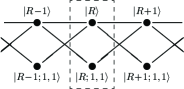
Figure 2: Effective lattice and effective unit cell for the configurations $\left|R\right\rangle$ and $\left|R;1,1\right\rangle$. The dashed box marks a primitive unit cell. The lines denote allowed tunneling between the configurations.

Instead of the $\cos{k}$-dispersion, we obtain the following $2\times 2$ matrix

$$H^{(2)}_{k}=-E_{J}\left(\begin{array}[]{cc}\cos{k}&\cos{k}\\[5.0pt] \cos{k}&0\end{array}\right)+\left(\begin{array}[]{cc}E_{0}&0\\[5.0pt] 0&E_{0}+E_{1,1}\end{array}\right)\ ,$$ (7)

where the second matrix accounts for the charging energies of the states $\left|R\right\rangle$ and $\left|R;1,1\right\rangle$. In what follows we omit the common energy $E_{0}$ for all states. Diagonalizing $H^{(2)}_{k}$ yields two bands as shown in Fig. 3 (blue dotted curves).

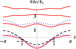
Figure 3: (Color online) Dispersion relation for the one-state-approximation, i.e., a single Cooper pair (black dashed band), for the two-state-approximation (blue dotted bands), and for the four-state-approximation (red solid bands) as described in the text. We chose $E_{C}=20E_{J}$, $\Lambda=10$.

Next we add the charge states $\left|\ldots 0\,1\,-1_{R}\,0\,1\,0\ldots\right\rangle\equiv\left|R;1,2\right\rangle$ and $\left|\ldots 0\,1\,0\,-1_{R}\,1\,0\ldots\right\rangle\equiv\left|R;2,1\right\rangle$. We find the $4\times 4$ tight binding matrix $H_{k}^{(4)}=$

$$\small-E_{J}\!\left(\begin{array}[]{cccc}\cos{k}&\cos{k}&\frac{1}{2}\exp{(-2ik)}&\frac{1}{2}\exp{(2ik)}\\[5.0pt] \cos{k}&-\frac{E_{1,1}}{E_{J}}&\frac{1}{2}&\frac{1}{2}\\[5.0pt] \frac{1}{2}\exp{(2ik)}&\frac{1}{2}&-\frac{E_{1,2}}{E_{J}}&\frac{1}{2}\exp{(ik)}\\[5.0pt] \frac{1}{2}\exp{(-2ik)}&\frac{1}{2}&\frac{1}{2}\exp{(-ik)}&-\frac{E_{1,2}}{E_{J}}\end{array}\right)\ .$$

In Fig. 3, the single particle band, the two bands of $H_{k}^{(2)}$, and the four bands of $H_{k}^{(4)}$ are shown for $E_{C}=20E_{J}$ and $\Lambda=10$. Here we are clearly in the strong Coulomb blockade regime and inclusion of the extra states only slightly modifies the lowest energy band.

The idea is now to approach the intermediate regime $\Lambda E_{J}>E_{C}>E_{J}$ by extending the number of charge configurations. Here we went up to the total width of the charge configurations $w_{c}=7$ resulting in a $32\times 32$ tight binding matrix. We investigate three regimes $E_{C}=10E_{J}$, $5E_{J}$, and $2.5E_{J}$ ($\Lambda=10$). The resulting spectra are shown in Fig. 4.

Figure 4: Band structure for $w_{c}=7$ with parameters $\Lambda=10$ and a) $E_{C}=10E_{J}$, b) $E_{C}=5E_{J}$, c) $E_{C}=2.5E_{J}$. For clarity, only the 16 lower bands are shown.

While in the strong Coulomb blockade regime $E_{C}>\Lambda E_{J}$ (see Fig. 3) the lowest band is very close to the $-cos{(k)}$ dispersion of a free particle, the shape of the lowest band in the regime of small solitons $E_{C}\leq\Lambda E_{J}$ (see Fig. 4) changes considerably. For $E_{C}/E_{J}=10$ which is the upper boundary of the ”small soliton” regime the lower band still has the cosine-shape for $|k|<\pi/2$. For larger values of $|k|$, however, the band becomes very flat which corresponds to zero group velocity or, equivalently, to infinite mass. For smaller ratios $E_{C}/E_{J}$, we find that the region in the center of the Brioullin-zone, which is cosine-like or parabolic, becomes smaller ($|k|<\pi/4$ for $E_{C}/E_{J}=2.5$). The remaining flat region shows a weak oscillatory behavior. We cannot exclude that it is due to an insufficient number of charge configurations included. Indeed, while for $E_{C}/E_{J}=10$ the numerical convergence for the lowest band is good, it somewhat deteriorates for smaller values of $E_{C}$. For $E_{C}=2.5E_{J}$ the first and second bands approach each other at $|k|\approx\pi/4$. This could give rise to Landau-Zener transitions for an accelerated soliton.

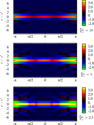
Figure 5: (Color online) Charge-charge correlator $\left\langle\psi_{k}\right|n_{r}n_{r^{\prime}}\left|\psi_{k}\right\rangle$ for $E_{C}=10E_{J}$, $5E_{J}$, and $2.5E_{J}$. In all plots $\Lambda=10$.

Soliton shape. We investigate the charge smearing in the regime of small solitons. For that purpose, we consider the charge-charge correlation function $F(k,r-r^{\prime})=\left\langle\psi_{k}\right|n_{r}n_{r^{\prime}}\left|\psi_{k}\right\rangle$, where $\left|\psi_{k}\right\rangle=\sum_{R,j}\alpha_{j}(k)\left|R,j\right\rangle e^{ikR}$ is the Bloch wave function of the soliton (lowest band). Here $\left|R,j\right\rangle$ denotes the $j$-th charge configuration centered at the island $R$, e.g., $\left|R\right\rangle$, $\left|R;1,1\right\rangle$, $\left|R;1,2\right\rangle$ etc.. We obtain $F(k,r-r^{\prime})=\sum_{j}\,|\alpha_{j}(k)|^{2}\,\mathcal{C}_{j}(r-r^{\prime})$, where $\mathcal{C}_{j}(r)\equiv\sum_{r^{\prime}}n^{R,j}_{r^{\prime}}n^{R,j}_{r^{\prime}+r}$ (this quantity is independent of R). The quantity $n^{R,j}_{r}$ is the number of charges on island $r$ for the charge configuration $\left|R,j\right\rangle$. Note that the correlation function is normalized, i.e., $\sum_{r^{\prime}}\langle n_{r}n_{r^{\prime}}\rangle=1$ if we choose the normalization of the Bloch wave functions such that $\sum_{j}|\alpha_{j}|^{2}=1$. In Fig. 5 we plot the charge-charge correlation function in the whole Brillouin zone. We observe extended structure appearing in the flat band regions. To characterize the width of the charge distribution we plot in Fig. 6 the quadrupole moment $\mathcal{Q}(k)=\sum_{r}{r}^{2}F(k,r)$. For small values of $k$ we observe the Lorentz contraction, as predicted by the sine-Gordon model. In the region of flat dispersion (infinite mass) the soliton becomes much wider. A question arises whether a model of sine-Gordon type could explain this phenomenon.

Discussion. In this paper, we have identified the regime of small charge solitons and investigated numerically their properties. One of the characteristic features is the flattening of the dispersion relation in the outer region of the Brillouin zone and simultaneous broadening of the soliton.

Our study was performed for infinite arrays with no disorder (offset charges). In the limit $\Lambda\gg 1$, both, the array borders and the offset charges create smooth variations of the potential energy of a Cooper pair (wells or barriers). The amplitude of these variations $\sim O(1)\Lambda E_{C}$ is, however, very large. The propagation of charge will thus crucially depend on the dispersion relations obtained in this paper as well as on the dissipation in the system. Further studies of these issues are necessary.

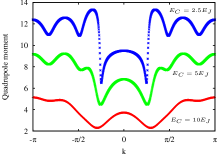
Figure 6: Quadrupole moment of the charge-charge correlator $\left\langle\psi_{k}\right|n_{r}n_{r^{\prime}}\left|\psi_{k}\right\rangle$ for $E_{C}=10E_{J}$, $5E_{J}$, and $2.5E_{J}$. For $|k|<\pi/4$ the Lorentz contraction can be observed.

We acknowledge numerous discussions with A. Ustinov, R. Schäfer, H. Rotzinger, and B. Malomed as well as the participants of the SCOPE 2009 meeting in Karlsruhe. We thank I. Martin for pointing Ref. BTB99 to us.

References

- (1) E. Ben-Jacob, K. Mullen, and M. Amman, Phys. Lett. A 135, 390 (1989).
- (2) D. V. Averin and K. K. Likharev, in Mesoscopic Phenomena in Solids, Vol. 30 of Modern Problems in Condensed Matter Sciences, edited by B. L. Altshuler, P. A. Lee, and R. A. Webb, (North-Holland, Amsterdam, 1991), Chap. 6, pp. 173 - 272.
- (3) A. Altland, L. I. Glazman, and A. Kamenev, Phys. Rev. Lett. 92, 026801 (2004).
- (4) Z. Hermon, E. Ben-Jacob, and G. Schön, Phys. Rev. B 54, 1234 (1996).
- (5) D. B. Haviland and P. Delsing, Phys. Rev. B 54, R6857 (1996).
- (6) D. B. Haviland, K. Andersson, and P. Ågren, J. Low Temp. Phys. 118, 733 (2000).
- (7) P. Ågren, K. Andersson, and D. B. Haviland, J. Low Temp. Phys. 124, 291 (2001).
- (8) A. B. Zorin, Phys. Rev. Lett. 96, 167001 (2006).
- (9) C. Hutter, A. Shnirman, Y. Makhlin, and G. Schön, Europhys. Lett. 74, 1088 (2006).
- (10) R. Fazio and G. Schön, Phys. Rev. B 43, 5307 (1991).
- (11) M. V. Fistul, V. M. Vinokur, and T. I. Baturina, Phys. Rev. Lett. 100, 086805 (2008).
- (12) S. V. Syzranov, K. B. Efetov, and B. L. Altshuler, Phys. Rev. Lett. 103, 127001 (2009).
- (13) J. Bonca, S. A. Trugman, and I. Batistic, Phys. Rev. B 60, 1633 (1999).