Violation of non-interacting $\cal V$-representability of the exact solutions of the Schrödinger equation for a two-electron quantum dot in a homogeneous magnetic field

Abstract

We have shown by using the exact solutions for the two-electron system in a parabolic confinement and a homogeneous magnetic field Taut-2einB ; Taut-3einB that both exact densities (charge- and the paramagnetic current density) can be non-interacting $\cal V$-representable (NIVR) only in a few special cases, or equivalently, that an exact Kohn-Sham (KS) system does not always exist. All those states at non-zero $B$ can be NIVR, which are continuously connected to the singlet or triplet ground states at $B=0$. In more detail, for singlets (total orbital angular momentum $M_{L}$ is even) both densities can be NIVR if the vorticity $\mbox{\boldmath$\gamma$}({\bf r})=\mbox{\boldmath$\nabla$}\times\Big{(}{\bf j}^{p}({\bf r})/n({\bf r})\Big{)}$ of the exact solution vanishes. For $M_{L}=0$ this is trivially guaranteed because the paramagnetic current density vanishes. The vorticity based on the exact solutions for the higher $|M_{L}|$ does not vanish, in particular for small r. In the limit $r\rightarrow 0$ this can even be shown analytically. For triplets ($M_{L}$ is odd) and if we assume circular symmetry for the KS system (the same symmetry as the real system) then only the exact states with $|M_{L}|=1$ can be NIVR with KS states having angular momenta $m_{1}=0$ and $|m_{2}|=1$. Without specification of the symmetry of the KS system the condition for NIVR is that the small-r-exponents of the KS states are 0 and 1.

I Introduction

Semi-relativistic Current-Density Functional Theory (CDFT) Vignale-Rasolt1 ; Vignale-Rasolt2 has become one on the standard tools for the calculation of electronic ground state (GS) properties in magnetic fields. Apart from the practical issue of finding an accurate and manageable energy functional, the basic fact of non-interacting $\cal V$-representability (NIVR) of the exact electron density $n({\bf r})$ and the paramagnetic current density $j^{p}({\bf r})$ is a prerequisite for the existence of a Kohn-Sham scheme. In a first step, we are investigating if both exact densities derived from the correlated two-particle state can be represented by the same set of one-particle orbitals

$$\varphi_{k}({\bf r})=R_{k}({\bf r})\;e^{i\zeta_{k}({\bf r})}$$ (1)

in the form (atomic units $\hbar=m=e=1$ are used throughout)

$$n({\bf r}) = \sum_{k}^{occ}\varphi_{k}^{*}({\bf r})\;\varphi_{k}({\bf r})=\sum_{k}^{occ}R_{k}^{2}({\bf r})$$ (2)

$${\bf j}^{p}({\bf r}) = \frac{1}{2i}\sum_{k}^{occ}\Big{[}\varphi_{k}^{*}({\bf r})\;\mbox{\boldmath$\nabla$}\varphi_{k}({\bf r})-\varphi_{k}({\bf r})\;\mbox{\boldmath$\nabla$}\varphi_{k}^{*}({\bf r})\Big{]}=\sum_{k}^{occ}R_{k}^{2}({\bf r})\;\mbox{\boldmath$\nabla$}\zeta_{k}({\bf r})$$ (3)

where the modulus $R_{k}({\bf r})\geq 0$ and the phase $\zeta_{k}({\bf r})$ of the Kohn-Sham wave-functions (KS-WF) are real functions. If the KS-WFs are well defined, then the effective potentials ${\cal V}^{eff}=(v^{eff}\;\mbox{and}\;{\bf A}^{eff})$ could be obtained from the KS equations as exercised in Ref.Wensauer-Roessler1 . In this paper we are only discussing if and when KS-WFs exist. Unlike in Density Functional Theory (DFT), NIVR in CDFT as defined above is neither guaranteed for nor restricted to GSs.

For vanishing magnetic field, DFT applies, which rests on some unique mappings. If $\Psi$ describes a many-body GS-WF and $n({\bf r})$ and $v^{ext}({\bf r})$ the corresponding density and external potential (modulo a constant), then of course $\Psi\stackrel{{\scriptstyle\cal D}}{{\rightarrow}}n({\bf r})$ is unique, but also $\Psi\stackrel{{\scriptstyle\cal C}}{{\rightarrow}}v^{ext}({\bf r})$ , if infinitely high potential walls are excluded. Hohenberg and Kohn HK proved that the mapping between $\Psi$ and $n({\bf r})$ is even one-to-one, and hence $n({\bf r})\;\stackrel{{\scriptstyle{\cal CD}^{-1}}}{{\longrightarrow}}v^{ext}({\bf r})$ is also unique

$$v^{ext}({\bf r})\;\;\stackrel{{\scriptstyle\cal C}}{{\leftarrow}}\;\Psi\;\;\begin{array}[]{c}{\scriptstyle\cal D}\\[-5.69054pt] \rightleftharpoons\\[-5.69054pt] {\scriptstyle{\cal D}^{-1}}\end{array}\;\;n({\bf r})$$ (4)

The situation of (4) holds for both the interacting and the non-interacting cases. For a NIVR density $n({\bf r})$, the mapping ${\cal CD}^{-1}$ for the non-interacting case yields the (effective) KS potential of the interacting system. It has been shown (e.g. in Levy ) that not every mathematically well behaved density $n({\bf r})$ is GS density to some potential $v^{ext}({\bf r})$. Therefore, DFT has been based on functionals which are also defined for non-$v$-representable densities. Nevertheless, a KS potential (derivative of the density functional) can only exist for NIVR densities.

In the presence of a magnetic field and for (semi-relativistic) Current Density Functional Theory (CDFT), the generalization of ${\cal D}^{-1}$ for the ground state still exists, but, Vignale and Rasolt Vignale-Rasolt1 ; Vignale-Rasolt2 just presupposed the existence of the generalization of $\cal C$ Capelle-Vignale1 implying that NIVR and the existence of a KS scheme has not been proven. Capelle and Vignale Capelle-Vignale1 , on the other hand, have shown that there can be several external potentials ${\cal V}^{ext}$ which provide the same wave functions and densities

$$\begin{array}[]{c}{\cal V}^{ext}_{1}({\bf r})\\ {\cal V}^{ext}_{2}({\bf r})\\ \cdots\end{array}\;\;\begin{array}[]{c}\searrow\\ \rightarrow\\ \nearrow\end{array}\;\;{\bf\Psi}\rightleftharpoons{\cal N}({\bf r})$$ (5)

where ${\cal V}^{ext}({\bf r})$ and ${\cal N}({\bf r})$ represent both external potentials ($v^{ext}({\bf r})$ and $\bf A^{ext}({\bf r})$) and both densities ($n({\bf r})$ and ${\bf j}^{p}({\bf r})$), respectively. Hence, $\cal C$ cannot exist anymore as a unique mapping. For Spin Density Functional Theory (SDFT) the same problem was first pointed out by von Barth and Hedin Barth-Hedin , and later analyzed in detail in Eschrig-Pickett1 ; Capelle-Vignale2 . For our model system the l.h.s. of (5) is obvious from the fact that the exact densities ${\cal N}({\bf r})$ are determined by the effective frequency

$${\widetilde{\omega}}=\sqrt{\omega_{0}^{2}+(\omega_{c}/2)^{2}}$$ (6)

alone and not by the external confinement frequency $\omega_{0}$ and the cyclotron frequency $\omega_{c}=B/c$ independently (see Sect.II). In other words, all combinations of $\omega_{0}$ and $\omega_{c}$, which provide the same $\widetilde{\omega}$, provide the same densities. This fact rules the existence of the mapping $\cal C$ out, but does neither prove nor rule out NIVR or the existence of a KS system.

Wensauer and Rössler Wensauer-Roessler1 used the scaling property of our quantum dot model system

$$H(\omega_{0},\omega_{c})=H(\omega_{0}\rightarrow{\widetilde{\omega}},\omega_{c}\rightarrow 0)+\frac{\omega_{c}}{2}\,L_{z}\;\;,$$ (7)

where $L_{z}$ is the total orbital angular momentum, in order to apply the consequences from the Hohenberg-Kohn theorem to non-zero fields. Indeed, (7) means that the Hamiltonian for a non-zero magnetic field $H(\omega_{0},\omega_{c})$ has the same eigen-functions as the Hamiltonian for zero magnetic field and the effective confinement frequency ${\widetilde{\omega}}$. Only the eigenvalues are shifted by $(\omega_{c}/2)M_{L}$, where $M_{L}$ is the total orbital angular momentum. The point is, however, that this does not mean that the GS densities ${\cal N}({\bf r})$ for all $\omega_{c}$ (for fixed $\omega_{0}$) are NIVR. Instead, this conclusion applies only to those cases, where the corresponding reference state at zero $\omega_{c}$ is a ground state. This are the states with $M_{L}=0$, which are special insofar, as the paramagnetic current vanishes even for non-zero magnetic field. Their argument does not say anything about NIVR of the other cases.

In the present paper we investigate, under which conditions the exact GS densities ${\cal N}({\bf r})$ of our model system can be represented by KS orbitals. For making the conclusions gauge independent, we also matched the gauge independent vorticity

$$\mbox{\boldmath$\gamma$}({\bf r})=\mbox{\boldmath$\nabla$}\times\frac{{\bf j}^{p}({\bf r})}{n({\bf r})}$$ (8)

instead of the paramagnetic current density ${\bf j}^{p}({\bf r})$. We will show that for a typical quantum dot model (two electrons in a parabolic confinement and a magnetic field) the exact GS densities are not generally NIVR. This is not a sophistry or subtleness, but the violation of NIVR is massive. This suffices to disprove the assumption of general NIVR and the general existence of a KS system for the GSs. On this background, all semi-relativistic CDFT calculations and functionals have to be considered with caution. On the other hand, this does not mean that all results are utterly wrong. However, this fact undermines the credibility of semi-relativistic CDFT as a tool for making forecasts.

II Specification of the model and exact densities

II.1 Model Hamiltonian

We consider a two-dimensional two-electron system (with Coulomb interaction between the electrons) in a harmonic scalar potential $v^{ext}(r)=(1/2)\;\omega_{0}^{2}\;r^{2}$ and a magnetic field perpendicular to the plane ${\bf B}=B\;{\bf e}_{z}$ represented by the vector potential (in symmetric gauge) ${\bf A}^{ext}({\bf r})=(1/2)\;{\bf B}\times{\bf r}=(1/2)\;B\;r\;{\bf e}_{\alpha}$. We introduced cylinder coordinates $(r,\alpha,z)$ with the cylinder axis perpendicular to the plane. The Hamiltonian reads

$$H=\sum\limits^{2}_{i=1}\biggl{\{}{1\over 2}\biggl{(}{\bf p}_{i}+{1\over c}{\bf A}^{ext}({\bf r}_{i})\biggl{)}^{2}+{1\over 2}\;\omega_{0}^{2}\;r_{i}^{2}\biggl{\}}+{1\over|{\bf r}_{2}-{\bf r}_{1}|}$$ (9)

This is a widely used effective Hamiltonian model for a two-electron quantum dot. The interaction of the spins with the magnetic field $H_{spin}=g^{*}\;\sum\limits_{i=1}^{3}\;{\bf s}_{i}\;\cdot{\bf B}$ is omitted (by chosing $g^{*}=0$) for two reasons. First, in semi-relativistic effective Hamiltonian theory $g^{*}$ is a material dependent parameter well below the vacuum value $g=2$. Therefore, the limiting case of vanishing $g^{*}$ ought to be covered by an exact theory. Second, the Zeeman term would make the Hamiltonian spin dependent and would necessitate a description of the system by the spin density $n_{s}({\bf r})$ (instead of the total density $n({\bf r}$)) and the paramagnetic current density ${\bf j}^{p}({\bf r})$ Vignale-Rasolt1 . The introduction of the spin density in SDFT produces its own problems Eschrig-Pickett1 ; Eschrig-Pickett2 ; Capelle-Vignale2 even for vanishing magnetic field, which we do not want to let interfere with the problems produced by the magnetic field.

II.2 Exact solutions of the Schrödinger equation

The Schrödinger equation with the Hamiltonian (9) can be solved not only by reduction to the numerical solution of an (ordinary) radial Schrödinger equation Merkt , but even analytically for a discrete, but infinite set of effective frequencies $\widetilde{\omega}$ Taut-2einB ; Taut-3einB . If we introduce relative and center of mass coordinate

$${\bf r}={\bf r}_{2}-{\bf r}_{1}~{}~{}~{}~{}~{};~{}~{}~{}~{}~{}{\bf R}={1\over 2}({\bf r}_{1}+{\bf r}_{2})$$ (10)

the Hamiltonian (9) decouples exactly.

$$H=2\;H_{r}+{1\over 2}\;H_{R}+H_{spin}$$ (11)

The Hamiltonian for the c.m. motion agrees with the Hamiltonian of a non-interacting quasi particle

$$H_{R}={1\over 2}\biggl{[}{\bf P}+{1\over c}{\bf A}_{R}\biggr{]}^{2}+{1\over 2}\omega_{R}^{2}\;R^{2}$$ (12)

and only the relative Hamiltonian contains the electron-electron interaction

$$H_{r}={1\over 2}\biggl{[}{\bf p}+{1\over c}{\bf A}_{r}\biggr{]}^{2}+{1\over 2}\omega_{r}^{2}\;r^{2}+\frac{1}{2r}\;\;,$$ (13)

where we introduced rescaled parameters $\omega_{R}=2\omega_{0}$, ${\bf A}_{R}=2{\bf A}({\bf R})$, $\omega_{r}={1\over 2}\omega_{0}$, ${\bf A}_{r}={1\over 2}{\bf A}({\bf r})$ (the index ’$r$’ and ’$R$’ refers to the relative and c.m. coordinate systems, respectively). The decoupling of $H$ allows the ansatz

$$\Phi=\xi({\bf R})\;\varphi({\bf r})\;\chi(s_{1},s_{2})$$ (14)

where $\chi(s_{1},s_{2})$ are the singlet or triplet spin eigen-functions.

The eigen-functions of the c.m. Hamiltonian (12) have the form

$$\xi={e^{iM\cal{A}}\over\sqrt{2\pi}}~{}~{}{U_{M}(R)\over R^{1/2}}=\frac{e^{iM\cal{A}}}{\sqrt{2\pi}}~{}~{}R_{M}(R)~{}~{}~{}~{}~{};~{}~{}~{}~{}~{}M=0,\pm 1,\pm 2,\ldots$$ (15)

where the polar coordinates of the c.m. vector are denoted by $(R,\cal{A})$ and the radial functions $U_{M}(R)$ and $R_{M}(R)$ can be found in standard textbooks.

With the following ansatz for the relative motion

$$\varphi={e^{im\alpha}\over\sqrt{2\pi}}~{}~{}{u_{m}(r)\over r^{1/2}}~{}~{}~{}~{}~{};~{}~{}~{}~{}~{}m=0,\pm 1,\pm 2,\ldots$$ (16)

the Schrödinger equation $H_{r}\,\varphi({\bf r})=\epsilon_{r}\,\varphi({\bf r})$ gives rise to a radial Schrödinger equation for $u(r)$

$$\biggl{\{}-{1\over 2}~{}{d^{2}\over dr^{2}}+{1\over 2}\biggl{(}m^{2}-{1\over 4}\biggr{)}{1\over r^{2}}+{1\over 2}\;\widetilde{\omega}_{r}^{2}\;r^{2}+\frac{1}{2r}\biggl{\}}u(r)=\widetilde{\epsilon}_{r}\;u(r)$$ (17)

where the polar coordinates for the relative vector are denoted by $(r,\alpha)$, $\widetilde{\omega}_{r}={1\over 2}\widetilde{\omega}$, $\widetilde{\epsilon}_{r}=\epsilon_{r}-{1\over 4}\,m\,\omega_{c}$, and $\omega_{c}={B\over c}$. The solutions are subject to the normalization condition $\int\limits^{\infty}_{o}dr|u(r)|^{2}=1$. The Pauli principle demands that (because of the particle exchange symmetry of the spin eigen-functions) in the singlet and triplet state, the relative angular momentum $m$ has to be even or odd, respectively. There is no constraint for the c.m. angular momentum $M$ following from Pauli principle. Because of the orthogonality of the coordinate transformation, the above described solutions are eigen-functions of the total orbital angular momentum with the eigenvalue $M_{L}=M+m$.

Fig.1 shows that the modulus of the orbital angular momentum of the ground state grows stepwise with increasing magnetic field. This implies that the spin state oscillates between singlet and triplet Merkt2 . (Quenching of the singlet state for higher magnetic fields due to a Zeeman term is not included in our model.) States with c.m. excitations are not included in the figure, because they are never ground states.

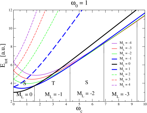
Figure 1: (color online) Total energy for fixed confinement frequency $\omega_{0}=1$ versus cyclotron frequency $\omega_{c}$ (i.e. magnetic field). The c.m. system is always in the ground state with $M=0$. The relative angular momentum $m$ is varied. The vertical lines show where the total orbital angular momentum $M_{L}=M+m$ of the ground state changes. S and T indicates whether the ground state is singlet or triplet. Thick lines indicate states which can be NIVR.

II.3 Exact densities

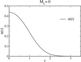
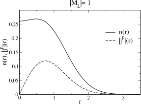
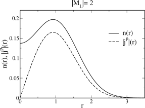
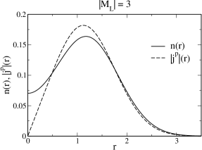
Figure 2: Exact densities and paramagnetic current densities (both in a.u.) for $\tilde{\omega}=1$ and the orbital angular momenta given in the titles of the figures. The sign of $j^{p}(r)$ agrees with the sign of $M_{L}$.

With (15) and (16), we obtain for the total density

$$n({\bf r})=2\int d{\bf r^{\prime}}\;|\Phi({\bf r},{\bf r^{\prime}})|^{2}$$ (18)

the general expression

$$n(r)=\frac{1}{2\pi^{2}}\int_{0}^{2\pi}d\alpha\int_{0}^{\infty}dr^{\prime}\;\bigg{[}R_{M}\Big{(}\sqrt{r^{2}+\frac{1}{4}r^{\prime 2}+rr^{\prime}cos\alpha}\Big{)}\bigg{]}^{2}\;\Big{[}u_{m}(r^{\prime})\Big{]}^{2}$$ (19)

Because we are interested in the ground state only, we can safely use the c.m. state for $M=0$: $R_{0}(R)=2\sqrt{\widetilde{\omega}}\;exp(-\widetilde{\omega}R^{2})$ which allows to do one integration analytically leaving us with

$$n(r)=\frac{4\widetilde{\omega}}{\pi}e^{-2\widetilde{\omega}\,r^{2}}\int_{0}^{\infty}dr^{\prime}\;e^{-(\widetilde{\omega}/2)r^{\prime 2}}\;I_{0}(2\widetilde{\omega}rr^{\prime})\Big{[}u_{m}(r^{\prime})\Big{]}^{2}$$ (20)

where $I_{n}(x)$ are the modified Bessel functions.

The general expression for the paramagnetic current density

$${\bf j}^{p}({\bf r})=-i\int d{\bf r^{\prime}}\;\Big{[}\Phi^{*}({\bf r},{\bf r^{\prime}})\mbox{\boldmath$\nabla$}\Phi({\bf r},{\bf r^{\prime}})-\Phi({\bf r},{\bf r^{\prime}})\mbox{\boldmath$\nabla$}\Phi^{*}({\bf r},{\bf r^{\prime}})\Big{]}$$ (21)

is somewhat complicated. Therefore we give here only the formula for $M=0$

$${\bf j}^{p}({\bf r})={\bf e}_{\alpha}\;m\;\frac{4\widetilde{\omega}}{\pi}e^{-2\widetilde{\omega}\,r^{2}}\int_{0}^{\infty}dr^{\prime}\;e^{-(\widetilde{\omega}/2)r^{\prime 2}}\;\frac{I_{1}(2\widetilde{\omega}rr^{\prime})}{r^{\prime}}\Big{[}u_{m}(r^{\prime})\Big{]}^{2}={\bf e}_{\alpha}\;j^{p}(r)$$ (22)

As to be expected, the paramagnetic current density points in azimuthal direction ${\bf e}_{\alpha}$, and the scalar $j^{p}(r)$ depends only on the distance $r$ from the center and not from the azimuthal angle .

Although both formulas (20) and (22) rely on the functions $u_{m}(r)$, which are solutions of (17), the analytical behavior for $r\rightarrow 0$ can be expressed in terms of two positive definite integrals

$$A_{0} = \int_{0}^{\infty}dr\;e^{-(\widetilde{\omega}/2)r^{2}}\;\Big{[}u_{m}(r)\Big{]}^{2}$$ (23)

$$A_{2} = \int_{0}^{\infty}dr\;r^{2}\;e^{-(\widetilde{\omega}/2)r^{2}}\;\Big{[}u_{m}(r)\Big{]}^{2}$$ (24)

After power series expansion of $I_{n}(x)$, we obtain

$$n(r) \rightarrow \frac{4\,\widetilde{\omega}}{\pi}e^{-2\,\widetilde{\omega}\,r^{2}}\Big{[}A_{0}+A_{2}\;\widetilde{\omega}^{2}\;r^{2}+\cdots\Big{]}$$ (25)

$$j^{p}(r) \rightarrow m\frac{4\,\widetilde{\omega}^{2}}{\pi}e^{-2\,\widetilde{\omega}\,r^{2}}\;r\Big{[}A_{0}+\frac{1}{2}A_{2}\;\widetilde{\omega}^{2}\;r^{2}+\cdots\Big{]}$$ (26)

For the origin this means that $n(0)=4\,\widetilde{\omega}\,A_{0}/\pi$ is always finite and $j_{p}(0)=0$ always vanishes. On the other hand, the derivative of the density at the origin $\frac{d\,n}{dr}(0)=0$ vanishes, but of the paramagnetic current density $\frac{d\,j_{p}}{dr}(0)=m(4\,\widetilde{\omega}^{2}/\pi)A_{0}$ is finite, unless $m=0$. Besides, there is a relation which does not rely on the radial functions at all

$$\frac{d\,j_{p}}{dr}(0)=m\;\widetilde{\omega}\;n(0)$$ (27)

The exact vorticity, which has the form $\mbox{\boldmath$\gamma$}({\bf r})={\bf e}_{z}\;\gamma(r)$, reads in this limit

$$\gamma(r)\rightarrow m\,2\;\widetilde{\omega}\;\Big{(}1-\widetilde{\omega}^{2}\;\frac{A_{2}}{A_{0}}\;r^{2}+\cdots\Big{)}$$ (28)

As will be seen below, the limit $r\rightarrow 0$ is decisive for our proof. The overall behavior of the densities is shown in Fig.2.

III Determine Kohn-Sham orbitals from exact density and paramagnetic current density

Our consideration is in a sense complementary to the approach in Wensauer-Roessler1 , where the triplet GS with $M_{L}=-1$ was considered. We are going to point out that this is the only triplet GS for which can be NIVR.

III.1 Singlet state:

In the KS system we assume that both electrons occupy the same orbital state of the form $\varphi({\bf r})=R({\bf r})\;e^{i\zeta({\bf r})}$ with different spins. We do not presuppose that this is an eigenstate of the orbital angular momentum, because there is no theorem which proves that orbital angular momentum is conserved in the KS system, if it is conserved in the real system. Now we demand that both densities ($n,{\bf j}^{p}$) in the KS and in the real system agree.

$$n_{KS}({\bf r})=2\;[R({\bf r})]^{2}\stackrel{{\scriptstyle!}}{{=}}n_{exact}(r)$$ (29)

$${\bf j}^{p}_{KS}({\bf r})=2\;[R({\bf r})]^{2}\;\mbox{\boldmath$\nabla$}\zeta({\bf r})\stackrel{{\scriptstyle!}}{{=}}j^{p}_{exact}(r)\;{\bf e}_{\alpha}$$ (30)

Equation (29) shows that the real part depends only on $r$ and reads

$$R(r)=\sqrt{\frac{1}{2}\;n_{exact}(r)}$$ (31)

Inserting the gradient in polar coordinates

$$\mbox{\boldmath$\nabla$}\zeta(r,\alpha)={\bf e}_{r}\;\frac{\partial\zeta}{\partial r}+{\bf e}_{\alpha}\;\frac{1}{r}\frac{\partial\zeta}{\partial\alpha}$$ (32)

into (30) and using (29) provides two equations for $\zeta(r,\alpha)$:

$$\frac{\partial\zeta(r,\alpha)}{\partial r}\stackrel{{\scriptstyle!}}{{=}}0\;\;\rightarrow\;\;\zeta=\zeta(\alpha)$$ (33)

$$\frac{\partial\zeta(\alpha)}{\partial\alpha}\stackrel{{\scriptstyle!}}{{=}}r\frac{j^{p}_{exact}(r)}{n_{exact}(r)}\equiv\mu_{exact}(r)\;\;\rightarrow\;\;\mu_{exact}(r)=const.$$ (34)

If a function of $\alpha$ has to agree with a function of $r$ (left equation of (34)), then both sides have to be a constant. Consequently, for NIVR the function $\mu_{exact}(r)$ has to be constant.

Before investigating this issue further, we introduce the vorticity (8) of the exact system. By using the special form of the $curl$ of a vector field $\bf v$, which points in ${\bf e}_{\alpha}$ direction and the modulus of which depends only on $r$,

$$\mbox{\boldmath$\nabla$}\times v(r)\,{\bf e}_{\alpha}=\frac{1}{r}\frac{d}{dr}\bigg{(}r\,v(r)\bigg{)}{\bf e}_{z}$$ (35)

we see that the vorticity of the exact solutions has the general form

$$\mbox{\boldmath$\gamma$}_{exact}({\bf r})=\frac{1}{r}\frac{d}{dr}\;\bigg{(}r\frac{j^{p}_{exact}(r)}{n_{exact}(r)}\bigg{)}\;{\bf e}_{z}\equiv\gamma_{exact}(r)\;{\bf e}_{z}$$ (36)

where ${\bf e}_{z}$ is the unit vector perpendicular to the 2D system, and from (34) it follows

$$\gamma_{exact}(r)=\frac{1}{r}\frac{d}{dr}\;\mu_{exact}(r)\stackrel{{\scriptstyle!}}{{=}}0$$ (37)

This means that for NIVR the exact vorticity $\gamma_{exact}(r)$ has to vanish.

The pure fact of violation of NIRV (without showing the quantitative extent in $r$-space) can already be seen analytically in the limit for small $r$ given in (28), which provides $\gamma_{exact}(0)=2\,{\widetilde{\omega}}\,M_{L}$. This value can be considered as a simple qualitative measure for the degree of violation. The numerical curves in Figs. 3 and 4 show that the violation of NIVR in an extented small-$r$-region is massive. There is only one singlet state, where NIVR is trivially guaranteed for all $r$. This is $M_{L}=0$, where the paramagnetic current and consequently $\mu_{exact}(r)$ and $\gamma_{exact}(r)$ vanish exactly. (As a side product we observe that $\mu_{exact}(r)$ converges for large $r$ to a constant, which agrees with the (total) orbital angular momentum $M_{L}$ of the exact state.)

Next we are investigating the vorticity of the KS system. From (8) and (29,30) it follows that the vorticity of one general KS state vanishes automatically

$$\mbox{\boldmath$\gamma$}_{KS}({\bf r})=\mbox{\boldmath$\nabla$}\times\mbox{\boldmath$\nabla$}\;\zeta({\bf r})=0$$ (38)

irrespective of its special form. If two electrons occupy the same orbital state then the density and paramagnetic current density have to be multiplied by the factor of 2 and the vorticity of the whole KS system vanishes automatically.

One could object that the above described procedure is not gauge invariant, because ${\bf j}^{p}({\bf r})$ is gauge dependent. If we replace (30) by equating the gauge invariant vorticities of both systems and consider that the vorticity of the (singlet state in the) KS system vanishes

$$\mbox{\boldmath$\gamma$}_{exact}({\bf r})\stackrel{{\scriptstyle!}}{{=}}\mbox{\boldmath$\gamma$}_{KS}({\bf r})=0$$ (39)

it is obvious that the exact vorticity has to vanish, what agrees with the result of the former approach. However, in order to be absolutely correct we have to consider the following subtlety. Observe that the canonical orbital angular momentum $\sum_{k}{\bf r}_{k}\times{\bf p}_{k}$ is gauge dependent and it is only conserved in the symmetric gauge (see Sect.IIA), which we used in out exact solutions. Therefore, we should characterize the only singlet state, which can be NIVR, in the following way: it is that state, which has $M_{L}=0$ in the symmetric gauge. This statement covers all gauges.

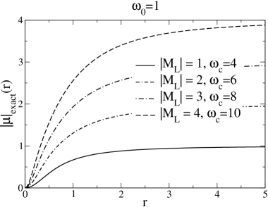
Figure 3: $\mu_{exact}(r)$ (in a.u.) for $\omega_{0}=1$ and typical cyclotron frequencies $\omega_{c}$, where the state with negative $M_{L}$ is the ground state (see Fig.1). The sign of $\mu_{exact}(r)$ agrees with the sign of $M_{L}$.

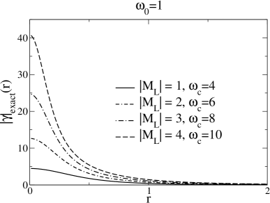
Figure 4: Vorticities (in a.u.) for the same external fields as Fig.3. The sign of $\gamma_{exact}(r)$ agrees with the sign of $M_{L}$.

III.2 Triplet state:

In a first step of sophistication we assume that the KS system is circular and the KS states are eigen-functions of the orbital angular momentum $\varphi_{k}({\bf r})=e^{im_{k}\alpha}R_{k}(r)$. (Do not mix up the relative angular momentum $m$ in in Sect.2 and the one-particle angular momentum $m_{k}$ in this section, which are both denoted by ’$m$’.) Therefore, we investigate, whether the exact system (which is circular and conserves total orbital angular momentum) can be replaced by a circular KS system with the same total angular momentum. This assumption is common practice in numerical self-consistent CDFT calculations and allows us to obtain the results in Ref.Wensauer-Roessler1 as a special case. Equating both densities $(n,{\bf j}^{p})$ provides the following set of equations

$$n_{KS}(r)=[R_{1}(r)]^{2}+[R_{2}(r)]^{2}\stackrel{{\scriptstyle!}}{{=}}n_{exact}(r)$$ (40)

$$j^{p}_{KS}(r)=m_{1}\frac{[R_{1}(r)]^{2}}{r}+m_{2}\frac{[R_{2}(r)]^{2}}{r}\stackrel{{\scriptstyle!}}{{=}}j^{p}_{exact}(r)$$ (41)

Now we investigate the limit for small $r$. In the Appendix it is shown that for the special case of a circular KS system $R_{k}(r)\rightarrow c_{k}\;r^{|m_{k}|}$. Equations (25) and (26) can be written as $n_{exact}(r)\rightarrow n_{0}+n_{2}\;r^{2}$ and $\j^{p}_{exact}(r)\rightarrow j_{0}\;M_{L}\;r$. Then (40) and (41) read in the limit $r\rightarrow 0$ for the essential lowest terms

$$c_{1}^{2}\;r^{2|m_{1}|}+c_{2}^{2}\;r^{2|m_{2}|}=n_{0}+n_{2}\;r^{2}$$ (42)

$$c_{1}^{2}\;m_{1}\;r^{2|m_{1}|-1}+c_{2}^{2}\;m_{2}\;r^{2|m_{2}|-1}=j_{0}\;M_{L}\;r$$ (43)

(42) can be fulfilled only if one of the angular momenta vanishes and the modulus of the other one is unity, say $m_{1}=0$ and $|m_{2}|=1$. This choice satisfies also (43). Consequently, only the exact states with $|M_{L}|=|m_{1}+m_{2}|=1$ can be NIVR by a circular KS system, whereby only the state with $M_{L}=-1$ can be the ground state (see Fig.1). In this case we obtain from (40) and (41) explicit formulae for the radial parts

$$[R_{2}(r)]^{2}=-r\;j^{p}_{exact}(r)$$ (44)

$$[R_{1}(r)]^{2}=n_{exact}(r)-[R_{2}(r)]^{2}$$ (45)

agreeing with Ref.Wensauer-Roessler1 .

In a second step, we abandon the constraint for circular symmetry of the KS system, because it cannot be taken for granted. Additionally, we equate the gauge invariant vorticities instead of the gauge-dependent paramagnetic current densities of the exact and the KS system. The analytical properties of the KS functions for $r\rightarrow 0$ in this general case are discussed in Appendix A. The gauge constants $m_{\cal G}$ can be neglected here because they cancel in gauge invariant quantities like $n({\bf r})$ and $\mbox{\boldmath$\gamma$}({\bf r})$ anyway. If we substitute $R_{k}(r)\rightarrow c_{k}\;r^{\widetilde{m}_{k}}$ in both KS densities (40) and (41), and insert both densities into the the vorticity of the KS system

$$\mbox{\boldmath$\gamma$}_{KS}({\bf r})=\mbox{\boldmath$\nabla$}\times\frac{{\bf j}^{p}_{KS}(r)}{n_{KS}(r)}\;{\bf e}_{\alpha}=\frac{1}{r}\frac{d}{dr}\,\bigg{(}r\,\frac{j^{p}_{KS}(r)}{n_{KS}(r)}\bigg{)}\;{\bf e}_{z}\equiv\gamma_{KS}(r)\;{\bf e}_{z}$$ (46)

we obtain

$$\gamma_{KS}(r)\rightarrow\frac{2\,c_{1}^{2}\;c_{2}^{2}\;(\widetilde{m}_{1}-\widetilde{m}_{2})^{2}\;r^{2(\widetilde{m}_{1}+\widetilde{m}_{2}-1)}}{[c_{1}^{2}\;r^{2\widetilde{m}_{1}}+c_{2}^{2}\;r^{2\widetilde{m}_{2}}]^{2}}$$ (47)

The lowest-power term of the exact vorticity (28) can be written as

$$\gamma_{exact}(r)\rightarrow\gamma_{0}\ M_{L}$$ (48)

Consequently, the two constraints from equating $n(r)$ and $\gamma(r)$ read

$$c_{1}^{2}\;r^{2\widetilde{m}_{1}}+c_{2}^{2}\;r^{2\widetilde{m}_{2}}=n_{0}+n_{2}\;r^{2}$$ (49)

$$\frac{2\,c_{1}^{2}\;c_{2}^{2}\;(\widetilde{m}_{1}-\widetilde{m}_{2})^{2}\;r^{2(\widetilde{m}_{1}+\widetilde{m}_{2}-1)}}{(n_{0}+n_{2}\;r^{2})^{2}}=\gamma_{0}\;M_{L}$$ (50)

whereby in the denominator of the second constraint the first constraint has been used. Although (50) and (43) differ, the conclusion from (42,43) and (49,50) are very similar. (49,50) can be fulfilled only if the small-r-exponents of the KS states are $0$ and $1$. The same conclusion can be drawn from equating the density and the paramagnetic current density for KS systems of arbitrary symmetry.

IV Summary and conclusions

We used the exact solutions of the Schrödinger equation of a two-dimensional model system for the investigation of NIVR. Qualitative conclusions can be drawn already on the basis of analytical results for the power expansion for $r\rightarrow 0$ of the densities ${\cal N}({\bf r})$.

For singlet states ($M_{L}=even$) there is a simple and straightforward proof without any assumptions that only the state with vanishing total orbital angular momentum $M_{L}=0$ can be NIVR. This state is the ground state for small magnetic fields (see Fig.1) and it does not produce a paramagnetic current.

For triplet states ($M_{L}=odd$) a fully satisfactory statement can be made only under the assumption, that the KS system has the same circular symmetry as the real system and consequently conserves orbital angular momentum. Then only the exact states with $|M_{L}|=1$ are NIVR by KS states with angular momenta $m_{1}=0$ and $|m_{2}|=1$.
If we allow KS systems with arbitrary symmetry, we can show that NIVR allows only KS states with small-r-exponents (see Appendix) of $0$ and $1$. However, we cannot say which exact states can or cannot be represented by symmetry-broken KS systems. In other words, we know that the exact states with $|M_{L}|=1$ can be represented by circular KS systems, and that all other states cannot be represented by circular KS systems. This statement is valuable despite its limitations, because the assumption of circular symmetry in self-consistent calculations is common practice.

At the end we want to discuss the connection between NIVR and the property of being a ground state. The singlet states belonging to the full black line ($M_{L}=0$) in Fig.1 can be NIVR, no matter whether they are ground states for the given $\omega_{0}$ and $\omega_{c}$ or not. All other states with even $M_{L}$ cannot, even if they are ground states. The full blue line ($M_{L}=-1$), which is the ground state in the second $\omega_{c}$-region in Fig.1, can be NIVR everywhere. Even the states belonging to the broken blue line ($M_{L}=+1$) are NIVR, although they are never the ground state. All other states with odd $M_{L}$ are not NIVR by a circular KS system. Consequently, all those states at non-zero $B$ can be NIVR, which are continuously connected to states at $B=0$, which are the ground states for a given spin state at $B=0$, no matter if they are the ground states at non-zero $B$ or not. The last statement sounds similar to the scaling property in Ref.Wensauer-Roessler1 , but it is not identical (see Introduction).

Appendix A General Kohn-Sham wave function for $\bf r\rightarrow 0$ and gauge dependence

We are going to show that (apart from a gauge-invariant normalization factor) any KS wave function in the limit $r\rightarrow 0$ has the form

$$\varphi_{KS}(r,\alpha)\rightarrow r^{\widetilde{m}}e^{i(\widetilde{m}+m_{\cal G})\alpha}$$ (51)

where the small-r-exponent $\widetilde{m}\geq 0$ is a gauge-invariant integer, but the integer $m_{\cal G}$ depends on the gauge. If the canonical angular momentum $l_{z}=(1/i)\partial/\partial\alpha$ is conserved, then $\widetilde{m}+m_{\cal G}$ is the canonical angular momentum $m$ of the KS state. Otherwise it is just a state and gauge-dependent integer. The limiting behavior of the density $n\rightarrow r^{2\widetilde{m}}$ is gauge-invariant, as expected, but the paramagnetic current density ${\bf j}^{p}\rightarrow(\widetilde{m}+m_{\cal G})\;r^{2\widetilde{m}-1}\,{\bf e}_{\alpha}$ depends on the gauge. Even if the canonical angular momentum is conserved, the exponent determining the radial WF (and the density) for small $r$ and the canonical angular momentum should not be mixed up.

The KS Hamiltonian has the general form

$$H_{KS}=\frac{1}{2}\biggl{[}\frac{1}{i}\mbox{\boldmath$\nabla$}+{1\over c}{\bf A}({\bf r})\biggr{]}^{2}+V({\bf r})$$ (52)

The concrete form of the effective potentials in this equation and their connection to the XC-energy functional can be found in Vignale-Rasolt2 . Now we apply a gauge transformation with $\chi=-c\,m_{\cal G}\,\alpha$ which changes the vector potential as follows

$${\bf A}\rightarrow{\bf A}^{\prime}={\bf A}+(\mbox{\boldmath$\nabla$}\chi)={\bf A}-c\;m_{\cal G}\,\frac{1}{r}\,{\bf e}_{\alpha}$$ (53)

This gauge transformation is equivalent to introducing a flux line with $m_{\cal G}$ flux quanta at the center. After rearranging terms and writing the Laplace operator in polar coordinates we obtain

$$H^{\prime} = -\frac{1}{2}r^{-1/2}\frac{\partial^{2}}{\partial r^{2}}r^{1/2}+\frac{1}{2\,r^{2}}\biggl{[}\bigg{(}\frac{1}{i}\frac{\partial}{\partial\alpha}-m_{\cal G}\bigg{)}^{2}-\frac{1}{4}\biggr{]}$$ (54)

$$+ \frac{1}{c}m_{\cal G}\,\frac{\bf A}{r}\cdot{\bf e}_{\alpha}+\frac{1}{2\,c}\frac{1}{i}(\mbox{\boldmath$\nabla$}\cdot{\bf A})+\frac{1}{c\,i}{\bf A}\cdot\mbox{\boldmath$\nabla$}+\frac{1}{2\,c^{2}}{\bf A}^{2}+V$$

Because in our model all external potentials are continuous, it is natural to assume that so is $V$ and $\bf A$. (Actually we have only to assume that $V$ diverges weaker than $1/r^{2}$ and $\bf A$ weaker than $1/r$.) Then the eigenfunction in the limit $r\rightarrow 0$ is defined by the first line in (54), which is independent of the specific form of $V$ and $\bf A$. With the ansatz

$$\varphi^{\prime}=\frac{u(r)}{r^{1/2}}\;w(\alpha)$$

and after multiplication with $r^{2}\,[1/u(r)w(\alpha)]\,r^{1/2}$ the variables in the Schrödinger equation $H^{\prime}\,\varphi^{\prime}=\epsilon\;\varphi^{\prime}$ can be separated providing

$$\frac{1}{u(r)}\biggl{[}-\frac{1}{2}r^{2}\frac{\partial^{2}}{\partial r^{2}}-r^{2}\epsilon\biggr{]}u(r)=\frac{1}{2}\frac{1}{w(\alpha)}\biggl{[}-\bigg{(}\frac{1}{i}\frac{\partial}{\partial\alpha}-m_{\cal G}\bigg{)}^{2}+\frac{1}{4}\biggr{]}w(\alpha)$$ (55)

This equation can only be fulfilled if both sides are constant. Using the technique of separation of variables, we can easily show that (51) is the solution, whereby the term with $r^{2}\,\epsilon$ on the l.h.s. can be neglected because we are interested in the limit $r\rightarrow 0$.

Acknowledgement

This work was supported by the German Research Foundation (DFG) in the Priority Program SPP 1145. We are indebted to K.Capelle and for valuable discussions and critically reading and improving the manuscript.

References

-
(1)
M. Taut, J. Phys. A27, 1045 (1994) and
J.Phys.A27, 4723 (1994) (erratum)
Additionally, in formula (8) the factor has to be replaced by , in formula (10) in the term containing a factor is missing, and on the r.h.s. of (19a) and (20a) must be replaced by .
For the technique for obtaining exact solutions see also: M.Taut, Phys.Rev.A48, 3561 (1993) -
(2)
M. Taut; J. Phys.: Condens. Matter 12, 3689 (2000)
misprints: in formula (21) the counter of the second term reads ,
in formula (73), has to be read as ,
and 4 lines before, in the definition of , has to be replaced by .
see also: M. Taut; Proceedings of the EP2DS Meeting, Ottawa 1999;
Physica E 6, 479 (2000) - (3) G.Vignale, M.Rasolt, Phys. Rev. B 37, 10685 (1988)
- (4) G.Vignale, M.Rasolt,Advances in Quantum Chemistry Vol.21, 235 (1990)
- (5) P.Hohenberg, W.Kohn, Phys. Rev. 136B, 864 (1964)
-
(6)
M.Levy, Phys.Rev.A 26, 1200 (1982)
H.English, R.English, Physica 121A, 253 (1983) - (7) K.Capelle, G.Vignale, Phys. Rev. B 65, 113106 (2002)
- (8) H.Eschrig, W.E.Pickett, Solid State Commun. 118, 123 (2001)
- (9) K.Capelle, G.Vignale, Phys. Rev. Lett. 86, 5546 (2001)
- (10) H.Eschrig, W.E.Pickett, J. Phys.: Condens. Matter 19, 315203 (2007)
- (11) U.von Barth, L.Hedin, J. Phys. C 5, 1629 (1972)
- (12) A.Wensauer, U.Rössler, Phys. Rev. B 69, 155301 and 155302 (2004)
- (13) U.Merkt, J.Huser and M.Wagner, Phys. Rev. B 43, 7320 (1991)
- (14) M.Wagner, U.Merkt and A.V.Chaplik, Phys. Rev. B 45, 1951 (1992)