Nonlinear Schrödinger Equation with Spatio-Temporal Perturbations

Abstract

We investigate the dynamics of solitons of the cubic Nonlinear Schrödinger Equation (NLSE) with the following perturbations: non-parametric spatio-temporal driving of the form $f(x,t)=a\,\exp[i\,K(t)\,x]$, damping, and a linear term which serves to stabilize the driven soliton. Using the time evolution of norm, momentum and energy, or, alternatively, a Lagrangian approach, we develop a Collective-Coordinate-Theory which yields a set of ODEs for our four collective coordinates. These ODEs are solved analytically and numerically for the case of a constant, spatially periodic force $f(x)$. The soliton position exhibits oscillations around a mean trajectory with constant velocity. This means that the soliton performs, on the average, a unidirectional motion although the spatial average of the force vanishes. The amplitude of the oscillations is much smaller than the period of $f(x)$. In order to find out for which regions the above solutions are stable, we calculate the time evolution of the soliton momentum $P(t)$ and soliton velocity $V(t)$: This is a parameter representation of a curve $P(V)$ which is visited by the soliton while time evolves. Our conjecture is that the soliton becomes unstable, if this curve has a branch with negative slope. This conjecture is fully confirmed by our simulations for the perturbed NLSE. Moreover, this curve also yields a good estimate for the soliton lifetime: the soliton lives longer, the shorter the branch with negative slope is.

I Introduction

The Nonlinear Schrödinger Equation (NLSE) is one of the paradigms of soliton physics, because it represents a completely integrable system and has very many applications in practically all fields of physics, which are listed and discussed in several review articles kivmal ; malo ; fadd . For applications it is important to study the perturbed NLSE

$$iu_{t}+u_{xx}+2|u|^{2}u=R[u(x,t);\,x,t].$$ (1)

Many different kinds of perturbations $R$ have been considered and in particular the dynamics of a single soliton under these perturbations was investigated kivmal ; malo .

In this paper we consider the following combination of perturbations

$$R=f(x,t)-i\beta u(x,t)-\delta u(x,t)$$ (2)

with the real parameters $\beta$ and $\delta$ and the non-parametric spatio-temporal driving force

$$f(x,t)=ae^{iK(t)\cdot x},$$ (3)

which yields several interesting effects, as we will see. The literature so far has mostly dealt with parametric driving kivmal ; malo ; bbk ; bbb ; scharf ; igor1 ; potabk . Non-parametric (external) driving was studied without space dependence, e. g., $f=\epsilon\exp(i\omega t)$ kaup ; bs ; bz , and with a periodic space dependence, e.g., $f=\epsilon\exp[i(kx-\omega t)]$ cohen ; vyas . Moreover, $f=\epsilon\exp[ig(x,t)-i\omega t]$, where $g$ is a function of $x-vt$, was considered, but no localized solutions were discussed vyas .

Our driving term in (3) was already used in the discrete form $f_{n}(t)=a\exp[in\phi(t)]$. Here the integer $n$ denotes a lattice site in a nonlinear optical waveguide array which is modeled by a Discrete Nonlinear Schrödinger Equation (DNLSE) gorbach . $\phi(t)$ is the incident angle of a laser beam. In order to obtain a ratchet effect, a biharmonic $\phi(t)$ was used which breaks a temporal symmetry.

In this paper we work with an arbitrary function $K(t)$ in the driving term (3) and develop a Collective Coordinate (CC) Theory for the soliton dynamics which results in a set of nonlinear coupled ODEs for the CCs (Sections II and III). In order to obtain analytical and numerical solutions we then consider the case of temporally constant, spatially periodic driving $f(x)=a$ exp $(iKx)$ with constant $K$ (Section IV). Although the spatial average of $f(x)$ vanishes, there is transport: the soliton performs a unidirectional motion on the average, in contrast to the case of the driving $R=V(x)u(x,t)$ with a periodic potential $V(x)$ in which the soliton performs an oscillatory motion around a minimum of $V(x)$ scharf . Solutions of the CC-Eqs. for the case of a harmonic or biharmonic time dependence of $K(t)$ will be presented in a second paper.

The second term, $-i\beta u(x,t)$ with $\beta>0$, in the perturbation (2) is a damping term which allows us to obtain a balance between the energy input from the driving and the dissipation. Other more complicated damping terms have been considered in mal93 ; komi0203 .

The third term, $-\delta u(x,t)$, in Eq. (2) will turn out to be decisive for the stability of the driven soliton. For $\delta\ \geq 0$ the soliton radiates phonons (i.e., linear excitations) and eventually vanishes, or even breaks up into several solitons. For $\delta<0$ the situation is more complicated and will be discussed below.

Section V presents a stable and an unstable stationary solution for the case without damping. For the region around the stable solution the CC-theory yields solutions in which all CCs exhibit oscillations with the same intrinsic frequency $\Omega$. However, tests by simulations, i.e. numerical solutions of the perturbed NLSE, reveal that the oscillatory solutions are stable only for certain regions of the initial conditions. These regions become broader when $\delta$ is more negative (Section VI).

We conjecture that the stability of any of these oscillatory solutions can be predicted by our CC-theory by calculating the curve $P(V)$, where $P(t)$ and $V(t)$ are the momentum and the velocity of the soliton, respectively. This means that every point on this curve is visited during one period of the oscillatory solution. The conjecture is that the soliton will become unstable in a simulation, if the curve $P(V)$ has a branch with negative slope, and this is confirmed by our simulations (Section VI). Interestingly, the curve $P(V)$ not only predicts whether the soliton is unstable, but it also allows us to estimate the soliton lifetime: This time is longer, the shorter the branch with negative slope is (Section VI).

The stability criteria for NLS-equations in the literature cannot be applied to our oscillatory solutions: The criterion of Vakhitov and Kolokolov vk ; w was established for stationary solutions, and the criterion of Barashenkov igor1 ; igor2 for solitons travelling with constant velocity. In igor1 ; igor2 the slope of a curve $\tilde{P}(\tilde{V})$, different from ours, is considered and decides about the stability. However, here each soliton solution is represented by one point on this curve, i.e. the curve represents a family of solutions with different velocities.

Finally we show in Section VII that the kinetic and canonical soliton momenta are identical, and we analytically calculate the soliton and phonon dispersion curves.

II Time evolution of norm, momentum, and energy

Multiplication of the perturbed NLSE (1) by $u^{*}$ and subtraction of the complex conjugate NLSE multiplied by $u$ yields

$$\frac{\partial\varrho}{\partial t}+\frac{\partial j}{\partial x}=i(R^{*}u-Ru^{*})$$ (4)

with the density and current density

$$\varrho=|u|^{2}\,,\,j=i(u^{*}_{x}u-u^{*}u_{x}).$$ (5)

By integration of Eq.(4) over $x$, assuming decaying boundary conditions, we obtain the time evolution of the norm,

$$N=\int^{+\infty}_{-\infty}dx|u|^{2}\,,$$ (6)

which is

$$\dot{N} = i\int^{+\infty}_{-\infty}dx(R^{*}u-Ru^{*})$$

$$= -2\beta N+i\int^{+\infty}_{-\infty}dx(f^{*}u-fu^{*})\,,$$ (7)

where the dot denotes the time-derivative and the terms with $\delta$ have dropped out.

Multiplication of Eq. (1) by $u_{x}^{*}$, addition of the complex conjugate equation multiplied by $u_{x}$, and integration over $x$ yields the time evolution of the momentum

$$\dot{P}=\int^{+\infty}_{-\infty}dx(R^{*}u_{x}+Ru_{x}^{*})$$ (8)

where $P$ is defined as

$$P=\frac{i}{2}\int^{+\infty}_{-\infty}dx(uu^{*}_{x}-u^{*}u_{x})\,.$$ (9)

Multiplication of Eq. (1) by $u^{*}_{t}$, addition of the complex conjugate equation multiplied by $u_{t}$, and integration yield the time evolution of the energy

$$\dot{E}=-\int^{+\infty}_{-\infty}dx(R^{*}u_{t}+Ru_{t}^{*})\,,$$ (10)

where

$$E=\int^{+\infty}_{-\infty}dx[|u_{x}|^{2}-|u|^{4}]\,.$$ (11)

Interestingly, for $\beta=0$ and time independent force, i. e. $R=f(x)-\delta u$, the r.h.s. of Eq. (10) can be written as a time derivative

$$\dot{E}=-\frac{\partial}{\partial t}\int^{+\infty}_{-\infty}dx[f^{*}u+fu^{*}-\delta|u|^{2}]\,.$$ (12)

Thus the perturbed NLSE (1) without damping possesses a conserved quantity for arbitrary $f(x)$

$$E^{tot}=\int^{+\infty}_{-\infty}dx[|u_{x}|^{2}-|u|^{4}-\delta|u|^{2}+f^{*}u+fu^{*}]\,.$$ (13)

$f(x)$ can be interpreted as a constant (external) force, in contrast to the case of the driving $R=V(x)u$, where $V(x)$ can be understood as a potential (in which the solitons move). In this case the conserved quantity is scharf (see also prlbishop )

$$E_{para}^{tot}=\int^{+\infty}_{-\infty}dx[|u_{x}|^{2}-|u|^{4}+V(x)|u|^{2}]\,.$$ (14)

In Sections IV and V we will show that a soliton under a constant periodic force $f(x)=a\exp(iKx)$ performs, on the average, a unidirectional motion, although the average of $f$ vanishes.

When we include the damping $(\beta>0)$, the time evolution of the total energy is

$$\dot{E}^{tot}=-\beta\int^{+\infty}_{-\infty}dx[2|u_{x}|^{2}-4|u|^{4}-2\delta|u|^{2}+f^{*}u+fu^{*}]\,.$$ (15)

III Collective Coordinate Theory

The 1-soliton solution of the unperturbed NLSE reads kivmal

$$u(x,t)=2i\eta\,\mathrm{sech}[2\eta(x-\zeta)]e^{-i(2\xi x+\phi)}$$ (16)

with the real parameters $\eta>0$ and $\xi$, the soliton position

$$\zeta(t)=\zeta_{0}-4\xi t\,,$$ (17)

and the phase of the internal oscillation

$$\phi(t)=\phi_{0}+4(\xi^{2}-\eta^{2})t\,.$$ (18)

The soliton has amplitude $2\eta$, width $1/(2\eta)$, velocity $V=-4\xi$ and phase velocity of the carrier wave $V_{ph}=-2\xi+2\eta^{2}/\xi$ .

Including the term with $\delta$ on the r.h.s. of Eq. (1), only the phase is changed:

$$\phi(t)=\phi_{0}+[4(\xi^{2}-\eta^{2})-\delta]t\,.$$ (19)

For this reason the term with $\delta$ need not be treated as a perturbation and will be counted among the unperturbed parts of the NLSE in the following

$$iu_{t}+u_{xx}+2|u|^{2}+\delta u=f(x,t)-i\beta u\,.$$ (20)

Therefore we now define the energy as

$$E=\int^{+\infty}_{-\infty}dx[|u_{x}|^{2}-|u|^{4}-\delta|u|^{2}]\,,$$ (21)

which is conserved for the unperturbed NLSE. Using Eq. (16) we obtain the soliton energy

$$E^{sol}=16\eta\xi^{2}-\frac{16}{3}\,\eta^{3}-4\delta\eta\,.$$ (22)

The definitions (6) and (9) need not be changed, because all terms with $\delta$ drop out on the r.h.s. of Eq. (7) and (8). The norm and the momentum of the soliton are, respectively,

$$N=4\eta\,;\,P=-8\eta\xi\,.$$ (23)

Writing $P=MV$, the soliton mass is related to the norm by $M=N/2$.

From the Inverse Scattering Theory (IST) it is well known kivmal that a perturbation theory results in a time dependence of $\eta$ and $\xi$ and in a change of the simple time dependence of $\zeta$ and $\phi$ in Eqs. (17) and (18). Therefore we take Eq. (16) as an ansatz with the four Collective Coordinates (CCs) $\eta(t),\xi(t),\zeta(t)$ and $\phi(t)$ (a similar ansatz has been used for optical solitons chaos ; komi04 ) and insert it into Eqs. (7), (8) and (10), using $f(x,t)=a\exp[iK(t)\cdot x]$ from Eq. (3).

Eq. (7) yields

$$\dot{\eta}=-2\beta\eta-a\frac{\pi}{2}\mathrm{sech}A\cdot\cos B,$$ (24)

with

$$A(t) = \frac{\pi}{4}[K(t)+2\xi(t)]/\eta(t),$$ (25)

$$B(t) = \phi(t)+[K(t)+2\xi(t)]\zeta(t)\,.$$ (26)

Two of the three terms which result on the r.h.s. of (8) cancel with the term $-8\dot{\eta}\xi$ on the l.h.s.. The remaining terms are

$$\dot{\xi}=aA\,\mathrm{sech}A\cdot\cos B\,.$$ (27)

Finally, Eq. (10) gives $8\eta\dot{\xi}\{...\}-4\dot{\eta}\{...\}=0$ with two different curly brackets. This equation can be fulfilled by setting both curly brackets to zero, which yields

$$\dot{\zeta} = -4\xi+\frac{a\pi^{2}}{8\eta^{2}}\mathrm{sech}A\cdot\tanh A\cdot\sin B,$$ (28)

$$\dot{\phi}+2\zeta\dot{\xi} = 4(\xi^{2}-\eta^{2})-\delta+\frac{a\pi A}{2\eta}\mathrm{sech}A\cdot\tanh A\cdot\sin B\,.$$ (29)

We can alternatively use the Lagrangian method which will also be useful for section VII. Our perturbed NLSE is equivalent to an Euler-Lagrange-Equation, generalized by a dissipative term,

$$\frac{d}{dt}\,\frac{\partial\mathcal{L}}{\partial u_{t}^{*}}+\frac{d}{dx}\,\frac{\partial\mathcal{L}}{\partial u_{x}^{*}}-\frac{\partial\mathcal{L}}{\partial u^{*}}=\frac{\partial\mathcal{F}}{\partial u_{t}^{*}},$$ (30)

with the Lagrangian density

$$\mathcal{L}=\frac{i}{2}(u_{t}u^{*}-u_{t}^{*}u)-|u_{x}|^{2}+|u|^{4}+\delta|u|^{2}-fu^{*}-f^{*}u,$$ (31)

and the dissipation function

$$\mathcal{F}=i\beta(uu_{t}^{*}-u^{*}u_{t})\,.$$ (32)

Inserting our CC-ansatz and integrating over the system we obtain the CC-Lagrangian

$$L=4\eta\dot{\phi}+8\eta\zeta\dot{\xi}-16\eta\xi^{2}+\frac{16}{3}\,\eta^{3}+4\delta\eta-2\pi a\,\mathrm{sech}A\cdot\sin B$$ (33)

and the CC-dissipation function

$$F=-\beta(8\eta\dot{\phi}+16\eta\zeta\dot{\xi})\,.$$ (34)

The CC-equations are then obtained by the four generalized Lagrange equations

$$\frac{d}{dt}\,\frac{\partial L}{\partial\dot{\psi}}-\frac{\partial L}{\partial\psi}=\frac{\partial F}{\partial\dot{\psi}},$$ (35)

where $\psi$ stands for the four CCs $\eta,\xi,\zeta$ and $\phi$. The resulting four ODEs are identical with the Eqs. (24), (27), (28) and (29).

Finally we evaluate Eq. (13), yielding

$$E^{tot}=16\eta\xi^{2}-\frac{16}{3}\eta^{3}-4\delta\eta+2\pi a\,\mathrm{sech}A\cdot\sin B\,.$$ (36)

Here the first three terms are the soliton energy (22), while the last term stems from the perturbations. We note that $E^{tot}$ is conserved only in the case of no damping $(\beta=0)$ and time independent force $f(x)=a\exp(iKx)$ with constant $K$, see below Eq. (12).

IV Constant, spatially periodic force

We consider this case because it exhibits some surprising, counter-intuitive features: E. g., the soliton position performs oscillations on a length scale that is very different from the spatial period $L$ of the force.

We take a constant $K$ in Eq. (3), i. e. $f(x)=a\exp(iKx)$, and consider only small values of $|K|$ such that the period $L=2\pi/|K|$ is much larger than the soliton width. We first consider the case with damping ($\beta>0$) for which we can expect “steady-state solutions” (see below Eq. (40)) for times much larger than a transient time $\tau$ on the order of $1/\beta$.

The transformation $u(x,t)=\Psi(X,t)\,\exp(iKx)$ into a moving frame $X=x-V_{f}t$ with $V_{f}=2\,K$ leads to the autonomous equation

$$i\Psi_{t}+\Psi_{XX}+2|\Psi|^{2}\Psi=a+(K^{2}-\delta)\Psi-i\beta\Psi,$$ (37)

with the non-parametric constant driving term $a$. Apart from the factor $K^{2}-\delta:=c^{2}$, which can be eliminated by scaling time by $c^{2}$, space by $c>0$, and $\Psi$ by $1/c$, Eq. (37) is the same as an autonomous equation, which was obtained from the NLSE (1) with $R=\epsilon\exp(i\omega t)-i\beta u$ by the substitution $u=\Psi(x,t)\exp(i\omega t)$, setting $\omega=1$ bs ; bz . However, these investigations differ from ours in several respects: In Ref. bs static soliton solutions of Eq. (37) were obtained numerically, then an existence and stability chart was constructed on the $(a,\beta)$ plane. In Ref. bz a singular perturbation expansion was performed at the soliton’s existence threshold. In contrast, we study moving solitons by solving our CC-equations, and test the results by simulations, i.e. by numerically solving the NLSE (1). Besides the steady-state solutions for $\beta>0$ (this section), for the case $\beta=0$ we study stationary solutions and oscillatory solutions, which have a more complicated time dependence (Section V).

The CC-equations from the previous section yield steady-state solutions, in which the driving is compensated by the damping, using the ansatz $\zeta=\zeta_{0}+V_{f}t$ with $V_{f}=2K$ and constant $\eta$, $\xi$, and $\phi$:

$$u_{f}^{\pm}(x,t)=2i\eta_{f}\mathrm{sech}\{2\eta_{f}[x-\zeta(t)]\}\mathrm{e}^{i(Kx-\phi_{f}^{\pm})},$$ (38)

with

$$\eta_{f} = \sqrt{K^{2}-\delta}/2,$$ (39)

$$\phi_{f}^{\pm} = \pm\frac{\pi}{2}+\,\arcsin\,\frac{4\beta\eta_{f}}{\pi a}.$$ (40)

We denote this as steady-state solutions, because $\phi$ is constant, in contrast to stationary solutions, where $\phi$ has a linear time dependence (Section V). These solitons have an internal structure due to the factor $\exp(iKx)$, but no internal oscillations since $\phi_{f}^{\pm}$ is constant. In the moving frame these solitons correspond to the above mentioned static solutions of Eq. (37) in Ref. bs .

We have numerically solved the CC-equations for many sets of initial conditions (IC) $\eta_{0},\zeta_{0},\xi_{0}$ and $\phi_{0}$. There is a basin of attraction around the solution (38) with $\phi_{f}^{+}$. The solitons always evolve to this solution, except when the values of $\eta_{0},\xi_{0}$ and $\phi_{0}$ are too far from those of this steady-state solution and when the damping $\beta$ is too large. An example for this is the parameter set $a=0.05$, $K=0.01$, $\delta=-3$, $\beta\geq\beta_{c}\approx 0.003$ with the IC $\eta_{0}=1$, $\xi_{0}=\zeta_{0}=\phi_{0}=0$. Here the soliton vanishes, i.e. its amplitude and energy go to zero while its width goes to infinity. In order to achieve a convergence to the stable steady-state solution one can either reduce $\beta$ below the critical value $\beta_{c}$ (which depends on the other parameters and the IC), or go closer to $\eta_{f}=0.8660$ by reducing $\eta_{0}$ by $0.1$, for instance, or go closer to $\phi_{f}^{+}$ by choosing $\phi_{0}=\pi/2$.

In this context it is interesting to consider the total energy (36) and its time derivative in which the CC-equations can be inserted. Using MATHEMATICA mathe we obtain

$$\dot{E}^{tot}(t)=-\beta\{8\eta[4(\xi^{2}-\eta^{2})-\delta]+4\pi A\,\mathrm{sech}A\cdot\tanh A\cdot\sin B\}\,.$$ (41)

This is indeed zero for the steady-state solution because $\xi_{f}=-K/2$ and thus $A\equiv 0$. On the path to that solution, Eq. (41) alternately exhibits both signs. I. e., the total energy performs oscillations which become smaller and smaller while approaching the final value $E^{tot}_{f}$.

According to Eq. (39), $\delta<K^{2}$. As we choose $|K|\ll 1$ (see above), $\delta$ is either positive but very small, or $\delta$ is negative. This results from the CC-theory; in section VII we will show that the driven soliton can be stable only for $\delta<0$, by taking into account the phonon modes.

The quality of the CC-theory must be tested by simulations. The soliton shape agrees very well (Fig. 1), but in the simulations the soliton resides on a small constant background because the perturbation $f(x)=a\exp(iKx)$ does not vanish far away from the soliton. This background is

$$u_{bg}=-\frac{a}{\omega_{K}}\,\mathrm{e}^{iKx},$$ (42)

with $\omega_{K}=K^{2}-\delta-i\beta$; see also the last term in Eq. (77). Plotting the real and imaginary parts of $u$, the spatial period $L=2\pi/|K|$ is observed. The norm density $|u|^{2}$ forms a shelf on which the soliton moves; the shelf height is quantitatively confirmed. The dynamics of the soliton is practically not affected by the background: the time evolution of the soliton position is identical in the CC-theory and the simulations (Fig. 2, right panel); only the soliton amplitude differs a little (left panel).

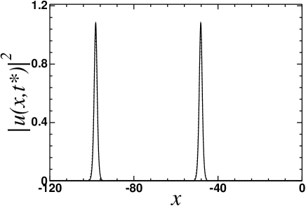
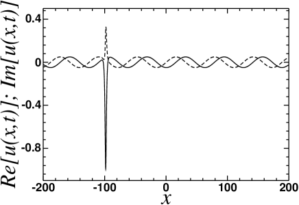
Figure 1: Left panel: Soliton moving to the left for $t^{*}=250,500$. Simulations of NLSE (solid lines) and numerical solutions of CC-equations (dotted lines). Right panel: Real (solid line) and imaginary (dashed line) parts of $u(x,t)$ for $t=500$. Parameters: $K=-0.1$, $a=0.05$, $\delta=-1$, $\beta=0.05$, with IC $\xi_{0}=0$, $\zeta_{0}=0$, $\phi_{0}=1.69$ and $\eta_{0}=0.5$.

All CCs exhibit decreasing oscillations with an intrinsic frequency $\Omega$ which will be discussed in the next section. However, oscillations are not visible in the soliton position $\zeta(t)$ in Fig. 2 because the linear term dominates the time evolution. By reducing the damping $\beta$ and by choosing a smaller time scale one can see the oscillations also in $\zeta(t)$, see Fig. 3.

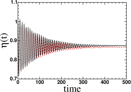
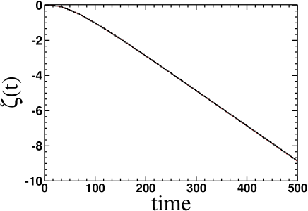
Figure 2: (Color online). The amplitude and position of the soliton obtained from a simulation of the NLSE (red dashed lines) and from the numerical solution of the CC equations (solid lines). Parameters: $K=-0.01$, $a=0.05$, $\delta=-3$, $\beta=0.01$, with IC $\xi_{0}=0$, $\zeta_{0}=0$, $\phi_{0}=\pi/2$ and $\eta_{0}=1$.

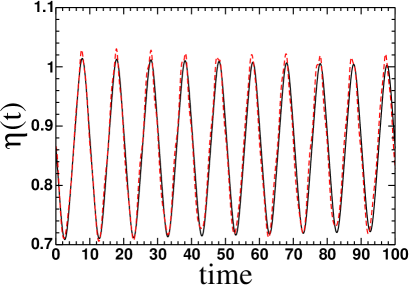
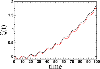
Figure 3: (Color online). The amplitude and position of the soliton obtained from a simulation of the NLSE (red dashed lines) and from the numerical solution of the CC equations (solid lines). Parameters: $K=0.1$, $a=0.05$, $\delta=-3$, $\beta=0.001$, with IC $\xi_{0}=0$, $\zeta_{0}=0$, $\phi_{0}=0$ and $\eta_{0}=\sqrt{K^{2}-\delta}/2$.

In any case, the soliton performs, on the average, a unidirectional motion although the spatial average of the periodic force $f(x)=a\,\exp(iKx)$ is zero. Thus, this is a ratchet-like system in which the translational symmetry is broken by the inhomogeneity $f(x)$ in the NLS-equation.

The period $L=2\pi/|K|$ of the inhomogeneity $f(x)$ is not reflected in the soliton dynamics, because our Eqs. (1)-(3) could be reduced to the autonomous Eq. (37). For early times $(t\leq\tau=O(1/\beta))$ the soliton performs the above mentioned oscillations. However, the amplitude of these oscillations is much smaller than $L$ (e.g., $L=62.8$ for $K=0.1)$. When the strength $a$ of the inhomogeneity is strongly increased $(a=1$, for instance), $\zeta(t)$ exhibits a staircase structure. The height of the steps is larger than the amplitude of the above oscillations, but still much smaller than $L$. However, such values of $a$ represent a strong perturbation for which the CC-theory can no longer be valid. Indeed, in the simulations the soliton soon becomes unstable.

V Oscillatory solutions

In order to study in more detail the intrinsic oscillations in the CCs (see previous section), we consider the case without damping $(\beta=0)$. Here oscillatory solutions are possible because the total energy (36) is conserved, see Eq. (41). This means that in Eq. (36) oscillations of the soliton energy, Eq. (22), are compensated by the oscillations of the term $2\pi a\,\mathrm{sech}A(t)\cdot\sin B(t)$ stemming from the perturbations. This is confirmed by inserting numerical solutions of the CC-equations into Eq. (36).

In order to obtain analytical solutions our approach is to look first for stationary solutions and then to consider small oscillations around them. For the stationary solutions we make the ansatz $\zeta=\zeta_{s}+V_{s}t,\eta=\eta_{s},\xi=\xi_{s}$ and $\phi=\phi_{s}-\alpha_{s}t$. The CC-equations (24), (27), (28), (29) yield

$$0 = -\frac{a\pi}{2}\,\mathrm{sech}A_{s}\cdot\cos B,$$ (43)

$$0 = aA_{s}\,\mathrm{sech}A_{s}\cdot\cos B,$$ (44)

$$V_{s} = -4\xi_{s}+\frac{a\pi^{2}}{8\eta^{2}_{s}}\,\mathrm{sech}A_{s}\cdot\tanh A_{s}\cdot\sin B,$$ (45)

$$-\alpha_{s} = 4(\xi_{s}^{2}-\eta^{2}_{s})-\delta+\frac{a\pi A_{s}}{2\eta_{s}}\,\mathrm{sech}A_{s}\cdot\tanh A_{s}\cdot\sin B,$$ (46)

with

$$A_{s} = \frac{\pi}{4}(K+2\xi_{s})/\eta_{s},$$ (47)

$$B(t) = \phi_{s}+(K+2\xi_{s})\zeta_{s}+[(K+2\xi_{s})V_{s}-\alpha_{s}]t\,.$$ (48)

Eq. (43) must be fulfilled for arbitrary $t$, thus $\cos B\equiv 0$, which leads to

$$\alpha_{s} = (K+2\xi_{s})V_{s},$$ (49)

$$\phi_{s}+(K+2\xi_{s})\zeta_{s} = \pm\frac{\pi}{2},$$ (50)

$$\sin B = \pm 1,$$ (51)

respectively. We distinguish two different cases: In case I, $\alpha_{s}=0$ and we obtain the steady-state solutions of Section IV. In the co-moving frame these solutions correspond to two exact static solutions of (37) for zero damping bs ; igor3 ; igor4 . Here one solution is stable below a critical driving strength, whereas the other one is always unstable.

In case II, $\alpha_{s}\neq 0$, which means that we obtain stationary solutions. Here we can restrict ourselves to the case $\zeta_{s}=\xi_{s}=0$, because other values yield qualitatively similar results. Using Eqs. (45), (46), (47) and (49) one transcendental equation for $\eta_{s}$ remains:

$$4\eta_{s}^{2}=-\delta\pm\frac{\pi^{2}aK}{4\eta_{s}^{2}}\mathrm{sech}A_{s}\cdot\tanh A_{s}.$$ (52)

For the parameter set $a=0.05$, $K=0.1$ and $\delta=-3$ we get $\eta_{s}=0.866239$ for $\phi_{s}=\pi/2$ and $0.865811$ for $\phi_{s}=-\pi/2$. The numerical solution of the CC-equations for these two cases reveals that in the former case we have a stable stationary solution, whereas in the latter case the solution is unstable.

For the region around the stable stationary solution we expect that all CCs exhibit oscillations and we assume that these oscillations are harmonic if the amplitudes are sufficiently small. We choose $\phi_{0}=\pi/2$ and make the ansatz

$$\zeta(t) = \bar{V}t-a_{\zeta}\,\sin(\Omega t),$$ (53)

$$\eta(t) = \eta_{0}+a_{\eta}\,[1-\cos(\Omega t)],$$ (54)

$$\xi(t) = -a_{\xi}\,[1-\cos(\Omega t)],$$ (55)

$$\phi(t) = \phi_{0}-\alpha t+a_{\phi}\sin(\Omega t).$$ (56)

This ansatz takes into account that the soliton first starts its oscillatory motion (i.e., $\zeta-\bar{V}t$ is linear in $t$ for small $t$), and then the soliton shape changes (i.e., $\eta$ is quadratic for small $t$).

Since we have considered the stationary solution that belongs to $\xi_{s}=\zeta_{s}=0$, we can neglect $\xi$ compared to $K$ and obtain for $B$ in Eq. (26):

$$B=\phi_{0}+(a_{\phi}-Ka_{\zeta})\sin(\Omega t)+(K\bar{v}-\alpha)t.$$ (57)

$Ka_{\zeta}$ is one order smaller than $a_{\phi}$, because $|K|\ll 1$, and we get

$$B=\phi_{0}+a_{\phi}\,\sin(\Omega t)+(K\bar{V}-\alpha)t.$$ (58)

Here we can distinguish two limiting cases: In case 1, the linear terms cancel and we have a pure oscillatory behavior. In case 2, the linear term dominates the oscillatory term which can then be neglected. Indeed, taking the second derivative of $\phi$ with respect to time and using (24), (27), (28) and (29) one obtains $\ddot{\phi}=c_{1}\sin(B)+c_{2}\sin(2\,B)+c_{3}\cos(B)+c_{4}\cos(2\,B)+c_{5}$, where $c_{i}$ with $i=1,2,...,5$ are functions of the CCs. Considering the above approximations, and in addition when the terms of order of $aK\bar{V}(4\eta_{0}^{2}+\delta)\,t$ are negligible, one realizes that $c_{1}$, $c_{2}$, $c_{4}$ and $c_{5}$ are small compared with $c_{3}=\Omega^{2}$,

$$\Omega^{2}\approx 4\pi a\eta_{0},$$ (59)

and hence, the Eq. for $\phi(t)$ reads

$$\ddot{\phi}-\Omega^{2}\cos(\phi)=0.$$ (60)

Integrating this equation once we obtain

$$\dot{\phi}=\pm\Omega\sqrt{2}\,\sqrt{\sin(\phi)+C},$$ (61)

where $C=\dot{\phi}^{2}_{0}/(2\,\Omega^{2})-\sin(\phi_{0})\approx((4\eta_{0}^{2}+\delta)^{2})/(8\pi a\eta_{0})-1$. Then, if $C\gg 1$, the constant term dominates and so $\phi(t)$ goes linearly, i.e. $\phi(t)=\pi/2\pm(4\,\eta_{0}^{2}+\delta)\,t$. Notice that $C\gg 1$ implies $(4\eta_{0}^{2}+\delta)^{2}\gg 16\pi a\eta_{0}$, which can be solved for $\eta_{0}$, yielding for $a=0.05$, $\delta=-3$ and $\phi_{0}=\pi/2$, $\eta_{0}\ll 0.655$ or $\eta_{0}\gg 1.077$. This is confirmed by numerical solutions of the CC-equations which exhibit an oscillatory behavior of $\phi(t)$ for $\eta_{0}\in[0.65;1.07]$, and a linear behavior (plus small oscillations) outside of this interval.

Finally we remark that in case II both $V_{s}$ in the stationary solutions and $\bar{V}$ in the oscillatory solutions differ from the value $2K$ in case I. A transformation to a frame moving with $V\neq 2K$ would not simplify the NLSE because terms with $\Psi_{X}$ would appear in Eq. (37).

VI Stability of oscillatory solutions

Our simulations reveal that the driven undamped soliton is stable only for a part of the set of solutions obtained by the CC-theory. Naturally we would like to predict, by using the CC-theory, which solutions are unstable and to understand what causes the instability. (The latter point will be discussed in the next section).

For the NLSE with a general local nonlinearity, but without driving and damping, the Vakhitov-Kolokolov stability criterion vk ; w states that solitons are stable if $dN/d\Lambda>0$. Here $N$ is the norm and $\Lambda$ the so-called spectral parameter in stationary solutions of the form $u(x,t)=\Psi(x)\exp(i\Lambda t)$. However, our oscillatory solutions, Eqs. (53)-(56) inserted into Eq. (16), have a more complicated time dependence than stationary solutions; therefore the criterion cannot be applied here.

The same holds for the stability criteria of Barashenkov igor1 ; igor2 which were established for solitons travelling with constant velocity. But here we can get some motivation for how to proceed in our case: Barashenkov showed that dark solitons of the NLSE with generalized nonlinearity are stable if $d\tilde{P}/d\tilde{V}<0$ (here the tildes are used to distinguish from our $P$ and $V$) igor2 . This proof was carried over to (bright and dark) solitons of the undamped parametrically driven NLSE igor1 . Here the point $d\tilde{P}/d\tilde{V}=0$ separates a stable from an unstable branch of the curve $\tilde{P}(\tilde{V})$, but it depends on the type of the solution on which side the stable branch is. For the following it is important to note that this curve $\tilde{P}(\tilde{V})$ represents a family of solutions with different velocities, i.e. each solution is represented by one point on the curve.

We make the conjecture that our oscillatory solutions are dynamically unstable, if our curve $P(V)$ has a branch with negative slope, i.e.

$$\frac{dP}{dV}<0,$$ (62)

for a finite interval of $V$. This curve is obtained from its parameter representation $P(t)$, $V(t)$, where $P(t)=-8\eta\xi$ is the soliton momentum Eq. (23) and the soliton velocity $V(t)=\dot{\zeta}$ is obtained by the r.h.s. of Eq. (28). Each oscillatory solution is represented by its own curve $P(V)$. This curve has a finite length, because $P(t)$ and $V(t)$ are periodic and remain finite, ($\zeta(t)$ and $\phi(t)$, which contain terms linear in $t$, do not appear in $P(t)$, and in $V(t)$ they appear only via $\sin B$, see Eq. (28)). Plotting the “stability curve” $P(V)$ we can inmediately see whether there is a branch with negative slope.

For the parameter set $a=0.05$, $K=0.1$, $\beta=0$ and $\delta=-1$ and IC $\zeta_{0}=\xi_{0}=0$ and $\phi_{0}=\pi/2$, we find a small “stability interval” $0.48\leq\eta_{0}\leq 0.52$, i.e. an interval of initial conditions for which the solutions are stable. As expected, this interval is situated around the value $\eta_{s}=0.501874$ from the stable stationary solution (52). There is another stable regime for $\eta_{0}\geq 0.76$. When we go far away from the IC for the stationary solution by choosing $\phi_{0}=0$, instead of $\phi_{0}=\pi/2$, the stability interval around $\eta_{s}$ vanishes. The upper stability regime exists now for $\eta_{0}\geq 0.69$.

When $|\delta|$ is increased, e.g. by choosing $\delta=-3$, the stability interval around $\eta_{s}=0.866239$ is much larger than in the case $\delta=-1$; for $\phi_{0}=\pi/2$ it is $0.7\leq\eta_{0}\leq 1.03$. The upper stability region is above $\eta_{0}=1.08$. Considering again $\phi_{0}=0$, the stability interval around $\eta_{s}$ only shrinks to $0.76\leq\eta_{0}\leq 0.97$, but does not vanish because it was much larger than in the case $\delta=-1$. The upper stable region is above $\eta_{0}=1.02$. Thus the conclusion is that an increase of $|\delta|$ widens the regions with stable soliton solutions. All the stability regions given above are confirmed by simulations for the perturbed NLSE, with an error of less than $1\,\%$.

At some of the boundaries of the above stability intervals there is a drastic change in the shape of the solutions of the CC-equations and the stability curve. E.g., if we choose $\eta_{0}=0.75$ (Fig. 4), which is just below the stability regime $\eta_{0}\geq 0.76$ (see above), we obtain very anharmonic oscillations in all CCs and the stability curve has a long branch with negative slope (Fig. 5). The simulations indeed show that the soliton becomes unstable very quickly and vanishes (Fig. 4). However, a slight change of $\eta_{0}$ to the value $0.76$ produces a stability curve that has only one branch with a positive slope (Fig. 5). Here the soliton is indeed stable in the simulations (Fig. 6).

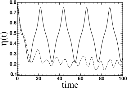
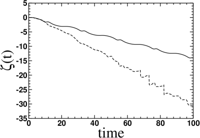
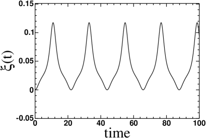
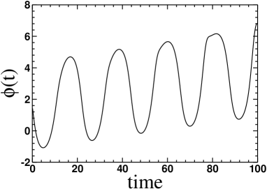
Figure 4: The evolution of $\eta$, $\zeta$, $\xi$ and $\phi$ obtained from a simulation of the NLSE (dashed lines) and from the numerical solutions of the CC equations (solid lines). Parameters: $K=0.1$, $a=0.05$, $\delta=-1$, $\beta=0$, with IC $\xi_{0}=0$, $\zeta_{0}=0$, $\phi_{0}=\pi/2$ and $\eta_{0}=0.75$.

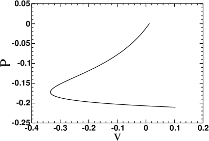
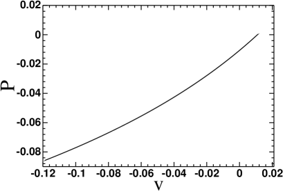
Figure 5: “Stability curve” $P$ versus $V$. Left panel: $\eta_{0}=0.75$. Right panel $\eta_{0}=0.76$. Other parameters as in Fig. 4.

At the boundaries of other stability intervals the change of the shape of the solutions is less dramatic. E.g., for the case $\delta=-1$ and $\eta_{0}=0.46$ the oscillations in the CCs are small and harmonic. The stability curve has only a very short branch with negative slope which is visited in the time evolution only for very short time intervals (Fig. 7). Here the soliton is indeed stable for a relatively long time (Fig. 8). This soliton lifetime is increasingly reduced when $\eta_{0}$ is reduced by which the negative slope branch in $P(V)$ becomes longer. Thus this curve predicts not only whether the soliton is stable, but also gives an estimate for its lifetime when it is unstable.

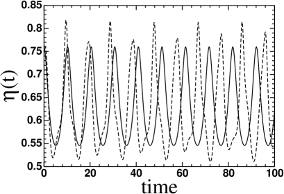
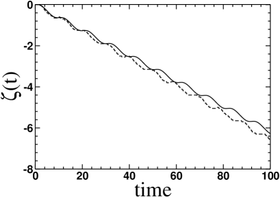
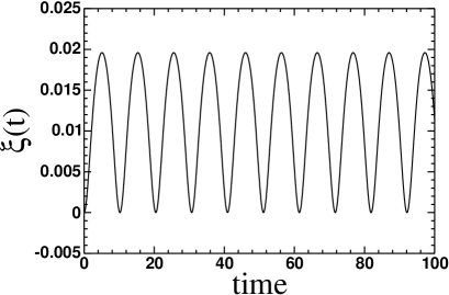
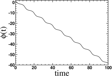
Figure 6: The evolution of $\eta$, $\zeta$, $\xi$ and $\phi$ obtained from a simulation of the NLSE (dashed lines) and from the numerical solutions of the CC equations (solid lines). Parameters: $K=0.1$, $a=0.05$, $\delta=-1$, $\beta=0$, with IC $\xi_{0}=0$, $\zeta_{0}=0$, $\phi_{0}=\pi/2$ and $\eta_{0}=0.76$. The simulations were carried forward to a final time $t_{f}=1000$.

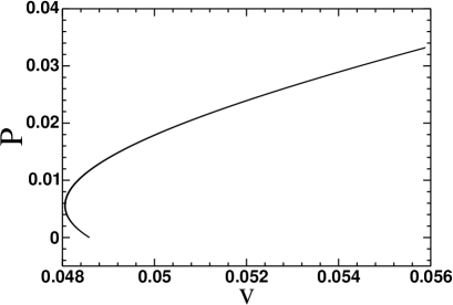
Figure 7: “Stability curve” close to the boundary of an unstable regime. Parameters: $K=0.1$, $a=0.05$, $\delta=-1$, $\beta=0$, with IC $\xi_{0}=0$, $\zeta_{0}=0$, $\phi_{0}=\pi/2$ and $\eta_{0}=0.46$.

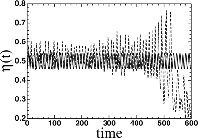
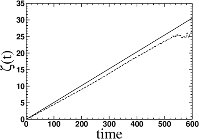
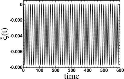
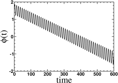
Figure 8: The evolution of $\eta$, $\zeta$, $\xi$ and $\phi$ obtained from a simulation of the NLSE (dashed lines) and from the numerical solutions of the CC equations (solid lines). Parameters as in Fig. 7.

VII Soliton and phonon dispersion curves

For the soliton dispersion curve $E^{sol}(P)$ we need the canonical momentum $P$ of the soliton. $P$ must fulfill the Hamilton equation

$$\dot{\zeta}=\frac{\partial H}{\partial P},$$ (63)

where $\zeta$ is the soliton position. We start from the CC-Lagrangian Eq. (33) and obtain

$$\frac{\partial L}{\partial\dot{\phi}}=4\eta=N,$$ (64)

as the angular momentum of the internal oscillation of the soliton, and

$$\frac{\partial L}{\partial\dot{\xi}}=8\eta\zeta=2N\zeta:=X,$$ (65)

as the variable which is canonically conjugate to $\xi$. Using a Legendre transformation we obtain the Hamilton function

$$H = X\dot{\xi}+N\dot{\phi}-L,$$ (66)

$$H(X,\xi;N,\phi) = 4N\xi^{2}-\frac{1}{12}N^{3}-\delta N+2\pi a\,\mathrm{sech}A\cdot\sin B,$$ (67)

with

$$A=2\pi\,\frac{K+2\xi}{2N},\qquad B=\phi+\frac{K+2\xi}{2N}\,X.$$ (68)

We now make an ansatz for a canonical transformation to the following new set of variables:

$$P = -2N\xi,\quad\zeta=\frac{1}{2\,N}\,X$$ (69)

$$\tilde{N} = N,\quad\tilde{\phi}=\phi+g(N,\xi,X).$$ (70)

This means that $P$ is identical to the kinetic momentum in Eq. (23), $\tilde{N}$ is chosen to be equal to $N$ and $g$ still has to be determined such that the four fundamental Poisson brackets are fulfilled. This yields $g=\xi X/N$. The new Hamiltonian reads

$$H(P,\zeta;N,\tilde{\phi})=\frac{1}{N}P^{2}-\frac{1}{12}N^{3}-\delta N+2\pi a\,\mathrm{sech}A\cdot\sin B,$$ (71)

with

$$A=\frac{\pi}{N}\,\left(K-\frac{P}{N}\right),\qquad B=\tilde{\phi}+K\zeta.$$ (72)

The first two terms in Eq. (71) agree with literature results on the unperturbed NLSE fadd . We have checked that the four Hamiltonian Eqs. which result from Eq.  (71) are indeed equivalent to the four CC-equations in section III for the case without damping. The above results hold for the force $f(x,t)$ in Eq. (3) with arbitrary $K(t)$. In the following we return to the case of constant $K$ in order to calculate analytically the stability and dispersion curves wherever it is possible.

Let us consider the stability intervals around the stationary solutions as given in Section VI. Except for the close vicinity to the boundaries of the stability intervals, the oscillations in the CCs are nearly harmonic and can be well approximated by the Eqs. (53) to (56). Inserting into $P=-8\,\eta\,\xi$, neglecting the 2nd harmonic, and using $V=\dot{\zeta}$, one can easily see that $P(V)$ is a straight line with slope

$$\frac{dP}{dV}=\frac{8\,\eta_{0}a_{\xi}}{\Omega\,a_{\zeta}}>0,$$ (73)

because for $\eta_{0}<\eta_{s}$ both $a_{\xi}$ and $a_{\zeta}$ are positive and for $\eta_{0}>\eta_{s}$ both are negative. The latter also holds for the upper stability intervals $\eta_{0}\geq 0.76$ for $\delta=-1$ and $\eta_{0}\geq 1.08$ for $\delta=-3$. Near or at the boundaries of the stability intervals, the oscillations in the CCs are very anharmonic and therefore the calculation leading to Eq. (73) is not possible. $P(V)$ is a curved line which can be calculated using the numerical solution of the CC-equations.

We now turn to the soliton dispersion curve $E^{sol}(P)$. Both $P=-8\,\eta\,\xi$ and $E^{sol}$ in Eq. (22) consist of powers of $\eta$ and $\xi$. For simplicity we write Eqs. (54) and (55) as $\eta=\bar{\eta}-a_{\eta}\,\cos(\Omega\,t)$ and $\xi=\bar{\xi}+a_{\xi}\,\cos(\Omega\,t)$, where $\bar{\xi}$ is negligible. We concentrate on the leading terms in $\cos(\Omega\,t)$ and distinguish two cases: In case I, both, $E^{sol}(t)$ and $P(t)$ have a leading term with $\cos(\Omega\,t)$; in this case the dispersion curve $E^{sol}(P)$ is linear in the first approximation. In case II, the $1^{st}$-order terms in $E^{sol}(t)$ cancel if $\bar{\eta}=\frac{1}{2}\,\sqrt{-\delta}$, but cannot cancel in $P(t)$. In the next order

$$E^{sol}(t)=E_{max}-\Delta E\,\cos^{2}(\Omega\,t),$$ (74)

with $\Delta\,E=16\,\bar{\eta}(a_{\eta}^{2}/3-a_{\xi}^{2})>0$ because $|a_{\xi}|\ll|a_{\eta}|$. Inserting $P=\bar{P}+8\bar{\eta}a_{\xi}\cos(\Omega\,t)$ yields a parabolic dispersion curve

$$E^{sol}(t)=E_{max}-\Delta E\,\left(\frac{P-\bar{P}}{8\,\bar{\eta}\,a_{\xi}}\right)^{2}.$$ (75)

This turns out to be a surprisingly good approximation when comparing with the dispersion curve obtained by using numerical solutions for $\eta(t)$ and $\xi(t)$, even when the cancellation of the linear terms in $E^{sol}(t)$ is not exact. The condition $\bar{\eta}=\sqrt{-\delta}/2$ is approximately fulfilled for the regions with strong oscillatory terms in $\phi(t)$; see end of Section V.

When solitons become unstable they radiate phonons (i.e., linear excitations). Therefore we consider the perturbed linearized NLSE without damping

$$iu_{t}+u_{xx}+\delta u=a\,e^{iKx},$$ (76)

which is solved by

$$u(x,t)=c\,e^{i(kx-\omega_{k}t)}+b\,e^{i(Kx-\omega_{K}t)}-\frac{a}{\omega_{K}}\,e^{iKx}$$ (77)

with $\omega_{k}=k^{2}-\delta$, $\omega_{K}=K^{2}-\delta$. The first term in Eq. (77) represents the phonons of the unperturbed equation with the free amplitude $c$ and the dispersion curve $\omega_{k}$.

The second term in Eq. (77) with the free amplitude $b$ represents a single phonon mode whose wave number and frequency are given by the parameter $K$ in the force $f(x)=a\,e^{iKx}$. Such phonons are typically radiated at the beginning of a simulation as the initial soliton profile adapts to the system. These phonons can be observed best when they interact with the soliton after having been reflected by a boundary of the system.

Finally, the last term in Eq. (77) represents a static background with a fixed amplitude $a/\omega_{K}$. This was already discussed below Eq. (42).

VIII Conclusions

We have considered the dynamics of NLS-solitons in one spatial dimension under the influence of non-parametric spatio-temporal forces of the form $f(x,t)=a\,\exp[i\,K(t)\,x]$, plus a damping term and a linear term $\delta\,u(x,t)$ which stabilizes the driven soliton. We have developed a CC-theory which yields a set of ODEs for the four CCs (position $\zeta$, velocity $\xi$, amplitude $\eta$, and phase $\phi$).

These coupled ODEs have been solved analytically and numerically for the case of a constant, spatially periodic force $f(x)=a\,\exp[i\,K\,x]$. The soliton position exhibits oscillations around a mean trajectory $\bar{\zeta}=\bar{V}\,t$; this means that the soliton performs, on the average, a unidirectional motion although the spatial average of the force vanishes. The amplitude of the oscillations is much smaller than the spatial period $L=2\pi/|K|$ of the inhomogeneity $f(x)$. The other three CCs also exhibit oscillations with the same frequency as $\zeta(t)$.

In the case of damping, the above oscillations are damped and the solution approaches a steady-state solution with constant velocity, if the IC are close enough to those of the steady-state solution and if the damping is not too large. Otherwise the soliton vanishes, i.e. its amplitude and energy go to zero while its width goes to infinity.

In the case without damping all the above oscillations persist. These periodic solutions exist because the total energy of the perturbed system is a conserved quantity, even for arbitrary inhomogeneity $f(x)$, and independent of the CC-ansatz.

However, a comparison with simulation results for the perturbed NLSE reveals that only part of the above oscillatory solutions are stable. Our CC-theory predicts the unstable regions in the IC and the parameter $\delta$ with high accuracy, by using our conjecture that the soliton becomes unstable if the slope of the curve $P(V)$ becomes negative somewhere: here $P(t)$ and $V(t)$ are the soliton momentum and velocity, respectively. It turns out that the stability intervals become broader when the parameter $\delta$ is chosen more negative. Moreover, we have found that the curve $P(V)$ also yields a good estimate for the soliton lifetime: The soliton lives longer, the shorter the negative-slope branch is, as compared to the length of the positive-slope branch.

Other cases of the force $f(x,t)=\exp[i\,K(t)\,x]$ will be considered in a second paper: specifically single and biharmonic $K(t)$, with and without damping.

IX Acknowledgments

We thank Yuri Gaididei (Kiev) and Igor Barashenkov (Cape Town) for very useful discussions on this work. F.G.M. acknowledges the hospitality of the University of Sevilla and of the Theoretical Division and Center for Nonlinear Studies at Los Alamos Laboratory. Work at Los Alamos is supported by the USDOE. F.G.M. acknowledges financial support from IMUS and from University of Seville (Plan Propio). N.R.Q. acknowledges financial support by the Ministerio de Educación y Ciencia (MEC, Spain) through FIS2008-02380/FIS, and by the Junta de Andalucía under the projects FQM207, FQM-00481 and P06-FQM-01735.

References

- (1) Y. Kivshar and B. Malomed, Rev. Mod. Phys. 61, 763 (1989).
- (2) B. Malomed, Prog. in Optics 43, 69 (2002).
- (3) L. D. Faddeev, L. Takhtajan, Hamiltonian methods in the theory of solitons, Classics in Mathematics, Springer-Verlag, Berlin (2007).
- (4) I. V. Barashenkov, M. M. Bogdan, and V. I. Korobov, Europhys. Lett. 15, 113 (1991).
- (5) M. Bondila, I. V. Barashenkov, and M. M. Bogdan, Physica D 87, 314 (1995).
- (6) I. V. Barashenkov, E. V. Zemlyanaya, and M. Bär, Phys. Rev. E 64, 016603 (2001).
- (7) R. Scharf and A. R. Bishop, Phys. Rev. E 47, 1375 (1993).
- (8) D. Poletti, E. A. Ostrovskaya, T. J. Alexander, B. Li, Y. S. Kivshar, Physica D 238, 1338 (2009).
- (9) D. J. Kaup and A. C. Newell, Proc. R. Soc. London A 361, 413 (1978), Phys. Rev. B 18, 5162 (1978).
- (10) I. V. Barashenkov, and Yu. S. Smirnov, Phys. Rev. E 54, 5707 (1996).
- (11) I. V. Barashenkov, and E. V. Zemlyanaya, Physica D 132, 363 (1999).
- (12) G. Cohen, Phys. Rev. E 61, 874 (2000).
- (13) V. M. Vyas, T. S. Raju, C. N. Kumar, and P. K. Panigrahi, J. Phys. A 39, 9151 (2006).
- (14) A. Gorbach, S. Denisov, and S. Flach, Opt. Lett. 31, 1702 (2006).
- (15) B. Malomed, Phys. Rev. E 47, 2874 (1993).
- (16) Y. Kominis and K. Hizanidis, J. Opt. Soc. Am. B, 19, 1746 (2002); ibid, 20, 545 (2003).
- (17) N. G. Vakhitov and A. A. Kolokolov, Radiophys. Quatum Electron. 16, 783 (1975).
- (18) M. I. Weinstein, Comm. Pure Appl. Math. 39, 51 (1986).
- (19) I. V. Barashenkov, Phys. Rev. Lett. 77, 1193 (1996).
- (20) For a DNLSE with , with , complete integrability for arbitrary was proven. D. Cai, A. R. Bishop, N. Gronbech-Jensen and M. Salerno, Phys. Rev. Lett. 74, 1186 (1995).
- (21) Akira Hasegawa, Chaos 10, 475 (2000).
- (22) Y. Kominis and K. Hizanidis, J. Opt. Soc. Am. B, 21, 562 (2004).
- (23) MATHEMATICA 5.2 (Wolfram Research Inc., Champaign.
- (24) I. V. Barashenkov, T. Zhanlav, and M. M. Bogdan, in “ Nonlinear World. IV International Workshop on Nonlinear and Turbulent Processes in Physics. Kiev, 9-22 October 1989”. Editors: V. G. Bar’yakhtar et al. World Scientific, 1990, pp. 3-9.
- (25) I. V. Barashenkov, Yu. S. Smirnov, and N. V. Alexeeva, Phys. Rev. E 57, 2350 (1998).