Electron-electron interactions in graphene bilayers

Electrons most often organize into Fermi-liquid states in which electron-electron interactions play an inessential role. A well known exception is the case of one-dimensional (1D) electron systems (1DES). In 1D the electron Fermi-surface consists of points, and divergences associated with low-energy particle-hole excitations abound when electron-electron interactions are described perturbatively. In higher space dimensions, the corresponding divergences occur only when Fermi lines or surfaces satisfy idealized nesting conditions. In this article we discuss electron-electron interactions in 2D graphene bilayer systems which behave in many ways as if they were one-dimensional, because they have Fermi points instead of Fermi lines and because their particle-hole energies have a quadratic dispersion which compensates for the difference between 1D and 2D phase space. We conclude, on the basis of a perturbative RG calculation similar to that commonly employed in 1D systems, that interactions in neutral graphene bilayers can drive the system into a strong-coupling broken symmetry state with layer-pseudospin ferromagnetism and an energy gap.

Recent progress in the isolation of nearly perfect single and multilayer graphene sheetsgraphene_reviews_1 ; graphene_reviews_2 ; graphene_reviews_3 ; graphene_reviews_4 has opened up a new topic in two-dimensional electron systems (2DES) physics. There is to date little unambiguous experimental evidence that electron-electron interactions play an essential role in the graphene family of 2DES’s. However, as pointed out by Min et al.min_prb_2008 graphene bilayers near neutrality should be particularly susceptible to interaction effects because of their peculiar massive-chiralmccann band Hamiltonian, which has an energy-splitting between valence and conduction bands that vanishes at ${\bm{k}}={\bm{0}}$ and grows quadratically with $k=|{\bm{k}}|$:

$${\cal H}_{B}=-\sum_{{\bm{k}}\sigma^{\prime}\sigma}\frac{\hbar^{2}k^{2}}{2m^{*}}c^{\dagger}_{{\bm{k}}\sigma^{\prime}}\big{[}\cos(J\phi_{\bm{k}})\tau^{x}_{\sigma^{\prime}\sigma}+\sin(J\phi_{\bm{k}})\tau^{y}_{\sigma^{\prime}\sigma}\big{]}c_{{\bm{k}}\sigma}.$$ (1)

In Eq. (1) the $\tau^{i}$s are Pauli matrices and the Greek labels refer to the two bilayer graphene sublattice sites, one in each layer, which do not have a neighbor in the opposite graphene layer. (See Fig. 1.) The other two sublattice site energies are repelled from the Fermi level by interlayer hopping and irrelevant at low energies. It is frequently useful to view quantum two-level layer degree of freedom as a pseudospin. The $J=2$ pseudospin chirality of bilayer graphene contrasts with the $J=1$ chiralitygraphene_reviews_1 ; chirality_correlations of single-layer graphene and is a consequence of the two-step process in which electrons hop between low-energy sites via the high-energy sites. The massive-chiral band-structure model applies at energies smaller than the interlayer hopping scalegraphene_reviews_4 $\gamma_{1}\sim 0.3~{}{\rm eV}$ but larger than the trigonal-warping scalegraphene_reviews_4 $\gamma_{3}\gamma_{1}/\gamma_{0}\sim 0.03~{}{\rm eV}$ below which direct hopping between low-energy sites plays an essential role. The body of this paper concerns the role of interactions in the massive-chiral model; we return at the end to explain the important role played by trigonal warping.

Figure 1: Bilayer graphene lattice structure and electronic structure. The massive chiral fermion model describes the low-energy sites in a AB-stacked graphene bilayer, those atom sites (top layer $B$ sites and bottom layer $A^{\prime}$ sites) which do not have a neighbor in the opposite layer. The conduction and valence bands touch at the Brillouin-zone corner wavevectors, taken as zero-momentum in continuum model theories, and separate quadratically with increasing wavevector. In a 1DES left and right going electrons cross the Fermi energy at a single point. In this figure the momentum of right-going (left-going) electrons is plotted relative to $+k_{F}$ ($-k_{F}$) where $k_{F}$ is the Fermi wavevector.

Similarities and differences between graphene bilayers and 1DES are most easily explained by temporarily neglecting the spin, and in the case of graphene also the additional valley degree of freedom. As illustrated in Fig. 1 in both cases the Fermi sea is point-like and there is a gap between occupied and empty free-particle states which grows with wavevector, linearly in the 1DES case. These circumstances are known to support a mean-field broken symmetry state in which phase coherence is established between conduction and valence band states for arbitrarily weak repulsive interactions. In the case of 1DES, the broken symmetry state corresponds physically to a charge density-wave (CDW) state, while in the case of bilayer graphenemin_prb_2008 it corresponds to state in which charge is spontaneously transferred between layers. This mean-field theory prediction is famously incorrect in the 1DES case, and the origin of the failure can be elegantly identifiedGiamarchi ; RGShankar using a perturbative renormalization group (PRG) approach. We show below that when applied to bilayer graphene, the same considerations lead to a different conclusion.

The reliability of the mean-field theory predictionmin_prb_2008 of a weak-interaction instability in bilayer graphene can be systematically assessed using PRGRGShankar . We outline the main steps in the application of this analysis to bilayer graphene in the main text, pointing out essential differences compared to the 1DES case. Details are provided in the supplementary material. We assume short-range interactions between electrons in the same ($S$) and different ($D$) layers.

The PRG analysis centers on the four point scattering function defined in terms of Feynman diagrams in Fig. 2. Since the Pauli exclusion principle implies that (in the spinless valleyless case) no pair of electrons can share the same 2D position unless they are in opposite layers, intralayer interactions cannot influence the particles; there is therefore only one type of interaction generated by the RG flow, interactions between electrons in opposite layers with the renormalized coupling parameter $\Gamma_{D}$. The direct and exchange first order processes in Fig. 2 have the values $V_{D}$ and $0$ respectively where $V_{D}$ is the bare coupling parameter.

The PRG analysis determines how $V_{D}$ is renormalized in a RG procedure in which fast (high energy) degrees of freedom are integrated out and the fermion fields of the slow (low energy) degrees of freedom are rescaled to leave the free-particle action invariant. The effective interaction $\Gamma_{D}$ is altered by coupling between low and high energy degrees of freedom. At one loop level this interaction is describedRGShankar by the three higher order diagrams labeled ZS, ZS’, and BCS in Fig. 2. The internal loops in these diagrams are summed over the high-energy labels. In the case of 1DES the ZS loop vanishes and the ZS’ and BCS diagrams cancel, implying that the interaction strengths do not flow to large values and that neither the CDW repulsive interaction nor the BCS attractive interaction instabilities predicted by mean-field theory survive the quantum fluctuations they neglect. The key message of this paper is summarized by two observations about the properties of these one-loop diagrams in the bilayer graphene case; i) the particle-particle (BCS) and particle-hole (ZS, ZS’) loops have the same logarithmic divergences as in the 1DES case in spite of the larger space dimension and ii) the ZS loop, which vanishes in the 1DES case, is finite in the bilayer graphene case and the BCS loop vanishes instead. Both of these changes are due to a layer pseudospin triplet contribution to the single-particle Green’s function as we explain below. The net result is that interactions flow to strong coupling even more strongly than in the mean-field approximation. The following paragraphs outline key steps in the calculations which support these conclusions.

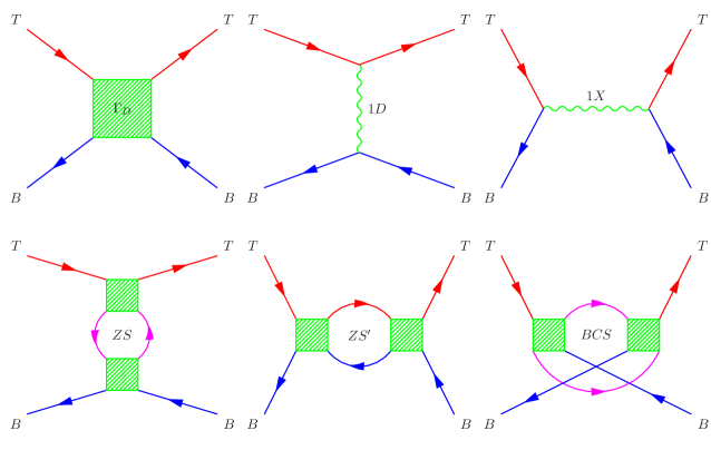
Figure 2: Four-point scattering function for bilayer graphene. The 1st diagram is the renormalized interaction while the 2nd and 3rd ones are the direct and exchange bare interactions, respectively. The following diagrams are the one-loop diagrams labelled ZS, ZS’ and BCS. The external and internal Green’s function labels refer to layer in the case of graphene and to chirality in the case of 1DES.

An elementary calculation shows that the single-particle Matsubara Green’s function corresponding to the Hamiltonian in Eq. (1) is

$${\mathscr{G}}({\bm{k}},i\omega_{n})=\left(\begin{array}[]{cc}{\mathscr{G}}_{\rm s}({\bm{k}},i\omega_{n})&-{\mathscr{G}}_{\rm t}({\bm{k}},i\omega_{n})e^{-iJ\phi_{\bm{k}}}\\ -{\mathscr{G}}_{\rm t}({\bm{k}},i\omega_{n})e^{iJ\phi_{\bm{k}}}&{\mathscr{G}}_{\rm s}({\bm{k}},i\omega_{n})\\ \end{array}\right)$$ (4)

where

$${\mathscr{G}}_{{\rm s},{\rm t}}({\bm{k}},i\omega_{n})\equiv{1\over 2}\left({1\over i\omega_{n}-\omega_{{\bm{k}}}}\pm{1\over i\omega_{n}+\omega_{\bm{k}}}\right),$$ (5)

and $\hbar\omega_{\bm{k}}=\xi_{\bm{k}}=\hbar k^{2}/2m^{*}$. The pseudospin-singlet component of the Green’s function ${\mathscr{G}}_{\rm s}$, which is diagonal in layer index, changes sign under frequency inversion whereas the triplet component ${\mathscr{G}}_{\rm t}$, which is off-diagonal, is invariant.

The loop diagrams are evaluated by summing the product of two Green’s functions (corresponding to the two arms of the Feynman diagram loops) over momentum and frequency. The frequency sums are standard and yield ($\beta=(k_{\rm B}T)^{-1}$)

$${1\over\beta\hbar^{2}}\sum_{\omega_{n}}{\mathscr{G}}_{{\rm s},{\rm t}}^{2}(i\omega_{n})=\mp{\tanh(\beta\xi_{\bm{k}}/2)\over 4\xi_{\bm{k}}}\mathop{\longrightarrow}\limits_{T\to 0}\mp{1\over 4\xi_{\bm{k}}}$$

$${1\over\beta\hbar^{2}}\sum_{\omega_{n}}{\mathscr{G}}_{\rm s}(i\omega_{n}){\mathscr{G}}_{\rm t}(i\omega_{n})\mathop{\longrightarrow}\limits_{T\to 0}0$$ (6)

where ${\bm{k}}$ is the momentum label shared by the Green’s functions. Note that the singlet-triplet product sum vanishes in the low-temperature limit in which we are interested. Each loop diagram is multiplied by appropriate interaction constants (discussed below) and then integrated over high energy momentum labels up to the massive chiral fermion model’s ultraviolet cutoff $\Lambda$:

$$\int_{\Lambda/s<k<\Lambda}\frac{d^{2}{\bm{k}}}{(2\pi)^{2}}\;\frac{\tanh(\beta\xi_{\bm{k}}/2)}{4\xi_{\bm{k}}}\;\mathop{\longrightarrow}\limits_{T\to 0}\;\frac{1}{2}{\nu_{0}}\,\ln(s)\,.$$ (7)

where $\nu_{0}=m^{*}/2\pi\hbar^{2}$ is the graphene bilayer density-of-states. Because $\omega_{\bm{k}}\propto k^{2}$, this integral grows logarithmically when the high-energy cut-off is scaled down by a factor of $s$ in the RG transformation, exactly like 1DES. This rather surprising property of bilayer graphene is directly related to its unusual band structure with Fermi points rather than Fermi lines and quadratic rather than linear dispersion.

The key differences between bilayer graphene and the 1DES appear upon identifying the coupling factors which are attached to the loop diagrams. The external legs in the scattering function Feynman diagrams (Fig. 2) are labeled by layer index ($T=$ top layer and $B=$ bottom layer) in bilayer graphene. The corresponding labels for the 1DES are chirality ($R=$ right-going and $L=$ left going); we call these interaction labels when we refer to the two cases generically. Since only opposite layer interactions are relevant, all scattering functions have two incoming particles with opposite layer labels and two outgoing particles with opposite layer labels. In the ZS loop, at the upper vertex the incoming and outgoing $T$ particles induce a $B$ particle-hole pair in the loop while the incoming and outgoing $B$ particles at the lower vertex induce a $T$ particle-hole pair. Since the particle-hole pairs must annihilate each other, there is a contribution only if the single-particle Green’s function is off-diagonal in interaction labels. This loop can be thought of as screening $V_{D}$; the sign of the screening contribution is opposite to normal, enhancing the bare interlayer interaction, because the polarization loop involves layer pseudospin triplet propagation. (See Eq. (Electron-electron interactions in graphene bilayers).) This contribution is absent in the 1DES case because propagation is always diagonal in interaction labels. The ZS’ channel corresponds to repeated interaction between a $T$ particle and a $B$ hole. This loop diagram involves only particle-propagation that is diagonal in interaction labels and its evaluation in the graphene bilayer case therefore closely follows the 1DES calculation. This is the channel responsible for the 1DES mean-field CDW instability in which coherence is established between $R$ and $L$ particles. In both graphene bilayer and 1DES cases it has the effect of enhancing repulsive interactions. The BCS loop corresponds to repeated interaction between the two incoming particles. In the 1DES case the contribution from this loop which enhances attractive interactions, cancels the ZS’ contribution, leading to marginal interactions and Luttinger liquid behavior. In the graphene bilayer case however, there is an additional contribution to the BCS loop contribution in which the incoming $T$ and $B$ particles both change interaction labels before the second interaction. This contribution is possible because of the triplet component of the particle propagation and, in light of Eq. (Electron-electron interactions in graphene bilayers), gives a BCS loop contribution with a sign opposite to the conventional one. Summing both terms, it follows that the BCS loop contribution is absent in the graphene bilayer case. These results are summarized in Table 1 and imply that at one loop level

$$\Gamma_{D}\simeq\frac{V_{D}}{1-V_{D}\nu_{0}\ln(s)}.$$ (8)

The interaction strength diverges when $V_{D}\,\nu_{0}=1/\ln(s)$, at half the mean-field theory critical interaction strength. Taking guidance from the mean-field theorymin_prb_2008 , the strong coupling state is likely a pseudospin ferromagnet which has an energy gap and spontaneous charge transfer between layers.

Table 1: Summary of contrasting the contributions (in units of the related density-of-states) of the three one-loop diagrams in 1DES and graphene bilayer cases

diagrams	ZS	ZS’	BCS	one-loop
1DES	$0$	$u^{2}\,\ln(s)$	$-u^{2}\,\ln(s)$	0
graphene bilayer	$\frac{1}{2}\,\Gamma_{D}^{2}\,\ln(s)$	$\frac{1}{2}\,\Gamma_{D}^{2}\,\ln(s)$	$0$	$\Gamma_{D}^{2}\,\ln(s)$

A number of real-world complications which have to be recognized in assessing the experimental implications of these results. First of all, electrons in real graphene bilayers carry spin and valley as well as layer pseudospin degrees of freedom. This substantially complicates the PRG analysis since many different types of interactions are generated by the RG flow. When one spin degree of freedom is considered three types of interactions have to be recognized, $\Gamma_{S}$, $\Gamma_{D}$, and $\Gamma_{X}$. $\Gamma_{S}$ couples electrons with the same flavor and $\Gamma_{D}$ electrons with different flavors, while $\Gamma_{X}$ is the exchange counterpart of $\Gamma_{D}$. The bare value of the exchange part of $\Gamma_{D}$ (the direct part of $\Gamma_{X}$) is of course zero since the Coulomb interaction is flavor independent, but higher order contributions are nonzero if triplet electron propagation is allowed. Correspondingly, when both spin and valley degrees of freedom are acknowledged the interaction parameters are $\Gamma_{SSD}$, $\Gamma_{SDS}$, $\Gamma_{SDD}$, $\Gamma_{DSS}$, $\Gamma_{DSD}$, $\Gamma_{DDS}$, $\Gamma_{DDD}$, $\Gamma_{XSD}$, $\Gamma_{XDS}$, and $\Gamma_{XDD}$ (see supplementary material) . The labels refer from left to right to sublattice pseudospin, real spin, and valley degrees of freedom. $\Gamma_{SSS}$ is absent due to Pauli exclusion principle while $\Gamma_{XSS}$ is just $-\Gamma_{DSS}$ due to the fermionic antisymmetry between outgoing particles. The one loop flow of these ten interaction parameters is described in the supplementary material. We find that the renormalized interactions diverge near $V_{D}\,\nu_{0}\simeq 0.6/\ln(s)$. The instability tendency is therefore somewhat enhanced by the spin and the valley degrees of freedom.

Next we must recognize that the massive chiral fermion model applies only between trigonal-warping and interlayer hopping energy scales. Appropriate values for $\ln(s)$ in the RG flows are therefore at most around $2.3$ (see supplementary material) in bilayer graphene, compared to the unlimited values of the chiral-fermion model. When combined with estimates of the bare interaction strengths (see supplementary material), this limit on interaction flow suggests that spontaneous gaps are likely in suspended bilayer graphene samples, and much less likely for graphene bilayers on substrates.

Gaps do appear in bilayer graphene even when electron-electron interactions are neglected, provided that an external potential difference $V$ is applied between the layers. The potential adds a single-particle term $-V\tau^{z}/2$ to the single-particle Hamiltonian, breaks inversion symmetry, and transfers chargeohta_science_2006 ; castro_prl_2007 ; SPBilayer_1 ; SPBilayer_2 between layers. This interesting property is in fact the basis of one strategy currently being explored in the effort to make useful electronic devicesoostinga_naturemat_2008 ; jens_MM_2009 out of graphene 2DES’s. Even if gaps do not appear spontaneously in real bilayer graphene samples, it is clear from the present work that interesting many-body physics beyond that captured by commonly used electronic-structure-theory approximations (LDA or GGA approximations for example), must play at least a quantitative role in determining gap grown with $V$. As graphene bilayer sample quality improves, we expect that it will be possible to explore this physics experimentally with ARPES, tunneling, and transport probes.

- (1) Ando, T. Theory of electronic states and transport in carbon nanotubes. J. Phys. Soc. Jpn. 74, 777-817 (2005).
- (2) Geim, A. K. & Novoselov, K. S. The rise of graphene. Nature Mater. 6, 183 (2007).
- (3) Geim, A. K. & MacDonald, A. H. Graphene: Exploring carbon flatland. Phys. Today 60(8), 35(2007).
- (4) Castro Neto, A. H., Guinea, F., Peres, N. M. R., Novoselov, K. S. & Geim, A. K. The electronic properties of graphene. Rev. Mod. Phys. 81, 109 (2009).
- (5) Min, H., Borghi, G., Polini, M. & MacDonald, A. H. Pseudospin magnetism in graphene. Phys. Rev. B. 77, 041407(R) (2008).
- (6) McCann, E. & Fal’ko, V. I. Landau-level degeneracy and quantum hall effect in a graphite bilayer. Phys. Rev. Lett. 96, 086805 (2006).
- (7) Barlas, Y., Pereg-Barnea, T., Polini, M., Asgari, R. & MacDonald, A. H. Chirality and correlations in graphene. Phys. Rev. Lett. 98, 236601 (2007).
- (8) Shankar, R. Renormalization-group approach to interacting fermions. Rev. Mod. Phys. 66, 129 (1994).
- (9) Giamarchi, T. Quantum Physics in One Dimension (Clarendon Press, Oxford, 2003).
- (10) Ohta, T., Bostwick, A., Seyller, T., Horn, K. & Rotenberg, E. Controlling the electronic structure of bilayer graphene. Science 313, 951 (2006).
- (11) Castro, E. V. et al., Biased bilayer graphene: semiconductor with a gap tunable by the electric field effect. Phys. Rev. Lett. 99, 216802 (2007).
- (12) McCann, E. Asymmetry gap in the electronic band structure of bilayer graphene. Phys. Rev. B, 74, 1403 (2006).
- (13) Min, H., Sahu, B., Banerjee, S.K. & MacDonald, A. H. Ab initio theory of gate induced gaps in graphene bilayers. Phys. Rev. B 75, 155115 (2007).
- (14) Oostinga, J. B., Heersche, H. B., Liu, X., Morpurgo, A. F. & Vandersypen, L. M. K. Gate-induced insulating state in bilayer graphene devices. Nature Mater. 7, 151 (2008).
- (15) Martin, J. Scanning single electron transistor microscopy on graphene. Bull. Am. Phys. Soc. 54 (1), 191 (2009).