Parallel Opportunistic Routing in Wireless Networks

Abstract

We study benefits of opportunistic routing in a large wireless ad hoc network by examining how the power, delay, and total throughput scale as the number of source–destination pairs increases up to the operating maximum. Our opportunistic routing is novel in a sense that it is massively parallel, i.e., it is performed by many nodes simultaneously to maximize the opportunistic gain while controlling the inter-user interference. The scaling behavior of conventional multi-hop transmission that does not employ opportunistic routing is also examined for comparison. Our results indicate that our opportunistic routing can exhibit a net improvement in overall power–delay trade-off over the conventional routing by providing up to a logarithmic boost in the scaling law. Such a gain is possible since the receivers can tolerate more interference due to the increased received signal power provided by the multi-user diversity gain, which means that having more simultaneous transmissions is possible.

I Introduction

In [1], Gupta and Kumar introduced and studied the throughput scaling in large wireless ad hoc networks. They showed that a total throughput scaling of $\Theta(\sqrt{n/\operatorname{log}n})$ [bps/Hz] can be obtained by using a multi-hop strategy when $n$ source-destination (S–D) pairs are randomly distributed in a unit area. Multi-hop schemes were then further developed and analyzed in the literature [3, 4, 5, 6, 7, 8, 9, 10] while their throughput per S–D pair scales far less than $\Theta(1)$. Recent studies [11, 12] have shown that we can actually achieve $\Theta(n^{1-\epsilon})$ scaling for an arbitrarily small $\epsilon>0$, i.e., an arbitrarily linear scaling of the total throughput, by using a hierarchical cooperation strategy, thereby achieving the best result we can hope for.

Besides the studies to improve the throughput up to the linear scaling, an important factor that we need to consider in practical wireless networks is the presence of multi-path fading. The effect of fading on the scaling laws was studied in [13, 6, 7, 3, 14], where it is shown that achievable scaling laws do not change fundamentally if all nodes are assumed to have their own traffic demands (i.e., there are $n$ S–D pairs) [13, 6, 7] or the effect of fading is averaged out [13, 6, 3], while it is found in [14] that the presence of fading can reduce the achievable throughput up to $\operatorname{log}n$. However, fading can be beneficial by utilizing the multi-user diversity (MUD) gain provided by the randomness of fading in multi-user environments, e.g., opportunistic scheduling [15], opportunistic beamforming [16], and random beamforming [17] in broadcast channels. Scenarios exploiting the opportunistic gain also studied in cooperative networks by applying an opportunistic two-hop relaying protocol [18] and in cognitive radio networks with opportunistic scheduling [19]. In [20, 21], strategies for improving the throughput scaling over non-faded environments were shown in wireless network models that do not incorporate geometric path loss. In [22], it was shown how fading improves the throughput using opportunistic routing when a single active S–D pair exists in a wireless ad hoc network.

In this paper, we analyze the benefits of fading by utilizing opportunistic routing in multi-hop transmissions when there are multiple randomly located S–D pairs in a large wireless ad hoc network. Our routing protocol describes how multiple nodes perform opportunistic routing simultaneously in a massive scale. To our knowledge, such an attempt for the network model has never been conducted in the literature. Since the throughput scaling of a multi-hop protocol is far less than linear, it is natural to assume that only a subset of S–D pairs are active at a time and active S–D pairs are chosen in a round robin fashion. In this paper, we consider a general scenario where the the number of active S–D pairs scales as a function of $n$. We are interested in improving the number of simultaneously supportable S–D pairs to maintain a constant throughput per S–D pair by using opportunistic routing.

In most network applications, power and delay are also key performance measures along with the throughput. The trade-off among these measures has been examined in terms of scaling laws in some papers [23, 8, 9, 10]. In this paper, we analyze a power–delay–throughput trade-off of both opportunistic routing and regular multi-hop routing as the number of S–D pairs increases up to the operating maximum, while per-node transmission rate is set to a constant. We first show the existence of a fundamental trade-off between the total transmission power consumed by all hops per S–D pair, the average number of hops per S–D pair, i.e., delay, and the number of active S–D pairs, which is proportional to the total throughput since we assume per-node transmission rate is a constant. It is investigated whether power can be reduced at the expense of increased delay for both routing scenarios, but a net improvement in overall power–delay trade-off can be obtained with opportunistic routing. The improvement comes from the MUD gain over the conventional multi-hop routing. This increases the average received signal power, which in turn makes it possible to have more simultaneous transmissions since more interference is tolerated while per-node transmission rate is maintained. More specifically, we show that such an MUD gain leads to a logarithmic performance improvement.

The rest of this paper is organized as follows. Section II describes our system and channel models. In Section III, our protocols with and without opportunistic routing are described. In Section IV, the power–delay–throughput trade-off for these protocols is analyzed and compared. Finally, Section V summarizes the paper with some concluding remarks.

II System and Channel Models

We consider a two-dimensional wireless network that consists of $n$ nodes uniformly and independently distributed on a square of unit area (i.e., dense network [1, 8, 9, 11]). We randomly pick S–D pairings such that each node is the destination of exactly one source. We assume that there are $M(n)$ randomly located S–D pairs, which can be active simultaneously, where $M(n)$ scales slower than $n$. Note that $M(n)$ sources can generate their own data traffic at the same time.

In this paper, to utilize the opportunistic gain, we adopt the physical channel model that can capture opportunism by modeling a realistic fading. The received signal $y_{k}$ at node $k\in\{1,\cdots,n\}$ at a given time instance is then given by

$$y_{k}=\sum_{i\in I}h_{ki}x_{i}+n_{k},$$

where $x_{i}\in\mathcal{C}$ is the signal transmitted by node $i$, $n_{k}$ is the circularly symmetric complex additive-white Gaussian noise with zero mean and variance $N_{0}$, and $I\subset\{1,\cdots,n\}$ is the set of simultaneously transmitting nodes. The channel gain $h_{ik}$ is given by

$$h_{ki}=\frac{g_{ki}}{r_{ki}^{\alpha/2}},$$ (1)

where $g_{ki}$ is the complex fading process between nodes $i$ and $k$, which is assumed to be Rayleigh with $E[|g_{ki}|^{2}]=1$ and independent for different $i$’s and $k$’s. Moreover, we assume the block fading model, where $g_{ki}$ is constant during one packet transmission and changes to a new independent value for the next transmission. $r_{ki}$ and $\alpha>2$ denote the distance between nodes $i$ and $k$ and the path-loss exponent, respectively. We assume that the channel state information (CSI) is available at all receivers, but not at the transmitters.

Throughout this paper $E[\cdot]$ denotes the expectation. Unless otherwise stated, all logarithms are assumed to be to the base 2.

III Routing Protocols

In this section, we describe our routing protocols with and without opportunistic routing. We simply use a multi-hop strategy in both cases using the nodes other than S–D pairs as relays. Hence, we do not assume the use of any sophisticated multi-user detection schemes at the receiver.

Next let us introduce the scaling parameters $P(n)$ and $D(n)$. The average number of hops per S–D pair is interpreted as the average delay and is denoted as $D(n)$. The parameter $P(n)$ denotes the average total transmit power used by all hops for an S–D pair. Assuming the transmit power is the same for each hop, we see that $P(n)$ is equal to $D(n)$ times the transmit power per hop. Since there is no CSI at the transmitter, we assume that each source node transmits data to its destination at a fixed target rate $R>0$ independent of $n$. A similar assumption was also made in some earlier works [1, 3, 4, 5, 6, 7, 8, 9, 10, 11, 12, 13, 14]. As in the earlier studies [15, 16, 17, 18, 19] dealing with opportunism under the block fading model, we suppose that a packet is decoded successfully if the received signal-to-interference-and-noise ratio (SINR) exceeds a pre-determined threshold $\eta>0$, which is independent of $n$, i.e., $\operatorname{log}(1+\text{SINR})\geq R=\operatorname{log}(1+\eta)$. Then, the total throughput $T(n)$ of the network would be given by $\Theta(M(n))$ if no transmission fails i.e., there is no outage. In addition, we scale all the transmit power such that the average total interference power from the set $I\subset\{1,\cdots,n\}$, consisting of simultaneously transmitting nodes, is given by $\Theta(1)$. Note that this strategy does not affect the trade-off among the orders of power $P(n)$, delay $D(n)$, and total throughput $T(n)$ (see Section IV-A for more detailed description).

III-A Opportunistic Routing

Opportunistic routing was originally introduced in [24, 25] and further developed in various network scenarios [26, 27, 28, 29]. When a packet is sent by a transmitter node, it may be possible that there are multiple receivers successfully decoding the packet. Among relaying nodes that successfully decode the transmitted packet for the current hop, the one that is closest to the destination becomes the transmitter for the next hop. Since the packet can travel farther at each hop using this opportunistic routing, the average number of hops can be reduced. Note that the existing protocol in [24, 25, 26, 27, 28, 29] was designed simply for the case where there exists a single S–D pair, and thus it did not incorporate interference between links, which is a critical problem in wireless networks.

We modify this routing to apply it to our network composed of multiple nodes performing opportunistic routing simultaneously in a massive scale. Then, we need to carefully design a routing protocol while solving the interference problem caused by simultaneously transmitting nodes. The per-hop distance of this opportunistic transmission is random. However, we can make sure that there are multiple successfully receiving nodes in a given square cell with high probability (whp) if we control the size of the cell and the distance between the transmitter and the cell. Then, one of the successfully receiving nodes can be the transmitter for the next hop. Short signaling messages [24, 25] need to be exchanged between some candidate relaying nodes and the corresponding transmit node in order to decide who will be the transmitter for the next hop. These messages are transmitted using a different time slot from that for data packets. More specifically, it is assumed that the two different messages are transmitted at even and odd time slots, respectively, which causes only a factor 2 loss in performance, thus resulting in no degradation in terms of scaling laws.

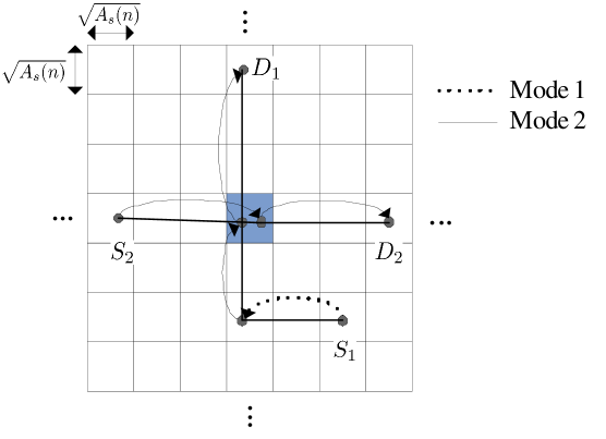
Figure 1: The S-D paths passing through the shaded cell.

As shown in Fig. 1, we divide the whole area into $1/A_{s}(n)$ square cells with per-cell area $A_{s}(n)$. Note that $A_{s}(n)=\Theta(1/D(n)^{2})$ holds since the average distance between an S–D pair is given by $\Theta(1)$. We assume XY routing, i.e., the route for an S–D pair consists of a horizontal and a vertical paths. Suppose that routing is performed first horizontally and then vertically for each S–D pair, as illustrated in Fig. 1 ($S_{i}$ and $D_{i}$ denote a source and the corresponding destination node, respectively, for $i=1,2$). Then, for each hop in the S–D path, some relay nodes that successfully decode their packets are selected opportunistically for transmission in the next hop (the relaying node selection strategy will be described later in detail). That is, the route for each S–D pair is not pre-determined. Nodes operate according to the 25-time division multiple access (TDMA) scheme. This means that the total time is divided into 25 time slots and nodes in each cell transmit 1/25-th of the time, while all transmitters in a cell transmit simultaneously. Figure 2 shows an example of simultaneously transmitting cells depicted as shaded cells.

Our routing protocol consists of two transmission modes, i.e., Modes 1 and 2, where Mode 2 is used for the last two hops to the destination and Mode 1 is used for all other hops (refer to Fig. 1 for the brief operation of two modes).

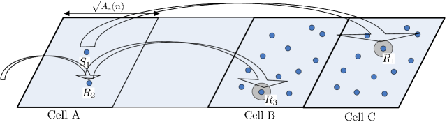
Figure 3: The opportunistic routing protocol in Mode 1.

Mode 1: We use an example in Fig. 3 to describe this mode. Transmitting nodes in Cell A transmit packets simultaneously, where one of those can be either source $S_{1}$ or relay node $R_{2}$. A relay node that successfully decodes the packet and is two (Cell B) or three (Cell C) cells apart from the transmitter horizontally (or vertically), for example $R_{1}$ or $R_{3}$ in Fig. 3, is arbitrarily chosen for the next hop. If there is no such node, then an outage occurs, i.e., none of the nodes satisfy $\text{SINR}\geq\eta$ in the cells. We do not assume any retransmission scheme in our case since we will make the outage probability negligibly small. If there are more than one candidate relay, then we choose one among them arbitrarily. Note that the MUD gain is roughly equal to the logarithm of the number of nodes in Cells B and C, which will be rigorously analyzed in the next section. We perform Mode 1 until the last two hops to the destination, and then switch to Mode 2. The reason we hop either two or three cells at a time is because 1) hopping to an immediate neighbor cell can create huge interference to a receiver node near the boundary of the two adjacent cells and 2) always hopping by two cells is not good since it partitions the cells into two groups, even and odd, and a packet can never be exchanged between the two groups.

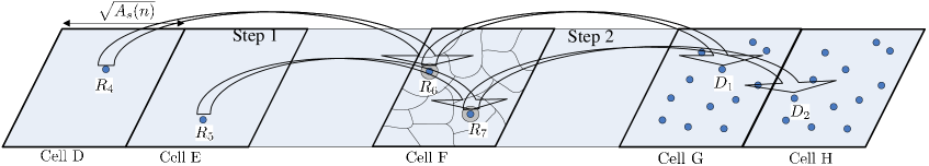
Figure 4: The opportunistic routing protocol in Mode 2.

Mode 2: For the last two hops to the destination, Mode 2 is used. If we use Mode 1 for the last hop, we cannot get any opportunistic gain since the destination is pre-determined. Hence, we use the following two-step procedure for Mode 2. We use the example in Fig. 4 to explain this mode.

• Step 1: In this step, a node in Cell D or E (e.g., $R_{4}$ or $R_{5}$ in Fig. 4) transmits its packet, whose signal reaches Cell F. This is similar to what happens in Mode 1 except that we are seeing this from Cell F’s perspective. Assuming $m$ nodes in Cell F, we arbitrarily partition Cell F into $\sqrt{m}$ sub-cells of equal size, i.e., there are roughly $\sqrt{m}$ nodes in each sub-cell. One node is then opportunistically chosen among the nodes that received the packet correctly in each sub-cell. Therefore, $\sqrt{m}$ nodes are chosen in Cell F as potential relays for the packet.

• Step 2: In Step 2, which corresponds to the last hop, the final destination in Cell G or H (e.g., $D_{1}$ or $D_{2}$ in Fig. 4) sends a probing packet, i.e., short signaling message, to see which one of the $\sqrt{m}$ selected relaying nodes in each cell will be the transmitter for the next hop whose channel link guarantees a successful packet transmission. Finally, the packet from the selected relaying node in cell F is transmitted to the final destination.

Although there are only $\sqrt{m}$ candidate nodes in each cell in Mode 2, whereas there were $m$ nodes in Mode 1, this does not affect the scaling law since the MUD gain is logarithmic in $m$ and $\operatorname{log}\sqrt{m}=\frac{1}{2}\operatorname{log}m$.

III-B Non-Opportunistic Routing

In this case, a plain multi-hop transmission [1, 8] is performed with a pre-determined path for each S–D pair consisting of a source, a destination, and a set of relaying nodes. Therefore, there is no opportunistic gain. The whole area is also divided into $1/A_{s}(n)$ cells with per-cell area $A_{s}(n)$ and one transmitter in a cell is arbitrarily chosen while transmitting at a fixed data rate $R>0$ independent of $n$. We assume the shortest path routing and the 9-TDMA scheme as in [1, 8]. However, even if interferences are carefully controlled, a transmission may fail due to fading, causing outages. In this paper, we simply assume that for the event that an outage occurs (i.e., $\operatorname{log}(1+\text{SINR})<R$) for a certain hop, such an event is not counted as outage, which will give an upper bound on the performance.

IV Power–Delay–Throughput Trade-off

Our goal in this section is to analyze the power–delay–throughput trade-offs with and without opportunistic routing. Provided that per-node transmission rate $R>0$ is given by a constant independent of $n$, we will show later that there exists a trade-off among scaling parameters $M(n)$, $P(n)$, and $D(n)$ for the two routing protocols we consider. By assuming the per-node rate of $R$, the trade-off among the four parameters $T(n)$, $M(n)$, $P(n)$, and $D(n)$ is thus essentially reduced to the trade-off among the three parameters $M(n)$, $P(n)$, and $D(n)$ such that any one of them can be changed freely, which in turn determines the other two. Note that with a constant rate $R$, the parameter $M(n)$ is proportional to the total throughput $T(n)$ since $T(n)=\Theta(M(n))$ if there is no outage. Note that different protocols will lead to different power–delay–throughput trade-offs.

If more power is available, then per-hop distance can be extended. Since the path-loss exponent $\alpha$ is greater than or equal to 2, the required power increases at least quadratically in the per-hop distance. On the other hand, the total power consumption of multi-hop is linear in the number of hops per S–D pair. Therefore, it seems advantageous to transmit to the nearest neighbor nodes if we want to minimize the total power. However, this comes at the cost of increased delay due to more hops. In the following subsections, we first show that there exists a fundamental trade-off between the total transmission power consumption per S–D pair, the average delay per S–D pair, and the total throughput, and then show that there is a net improvement in the overall power–delay tradeoff when our opportunistic routing is utilized in the network.

IV-A Opportunistic Routing

The relationship among the three parameters $M(n)$, $P(n)$, and $D(n)$ is derived under the opportunistic routing described above. More specifically, we are interested in how many S–D pairs, denoted by $M(n)$, can be active simultaneously while maintaining a constant transmission rate $R$ per S–D pair. In the following, we mainly focus on Mode 1 since Mode 2 can be similarly analyzed with a slight modification. First let $\text{SINR}_{k(m,l_{m})}^{l_{m}}$ denote the SINR value seen by receiver $k(m,l_{m})$ for the $l_{m}$-th hop of the $m$-th S–D pair, where $l_{m}\in\mathcal{H}_{m}$ and $m\in\{1,\cdots,M(n)\}$. Here, $\mathcal{H}_{m}=\{1,2,\cdots,d_{m}D(n)\}$ denotes the set of hops for the $m$-th S–D path, where $d_{m}$ is a positive parameter that scales as $O(1)$. Let $N_{c}(n)$ denote the number of nodes in each cell. Then it follows that $k(m,l_{m})\in\{1,\cdots,2N_{c}(n)\}$ since two cells are taken into account for selecting one receiver node. Note that for each hop, a receiver is either two or three cells apart from the transmitter. Then, we have

$$\text{SINR}_{k(m,l_{m})}^{l_{m}}=\frac{P_{r}^{k(m,l_{m})}}{N_{0}+P_{I}^{k(m,l_{m})}},$$ (2)

where $P_{r}^{k(m,l_{m})}$ and $P_{I}^{k(m,l_{m})}$ denote the received signal power at node $k(m,l_{m})$ from the desired transmitter $i(m,l_{m})$ for the $l_{m}$-th hop of the $m$-th S–D pair and the total interference power at node $k(m,l_{m})$ from all interfering nodes, respectively. Specifically, they are given by

$$P_{r}^{k(m,l_{m})}=|h_{k(m,l_{m})i(m,l_{m})}|^{2}\frac{P(n)}{D(n)}$$ (3)

and

$$P_{I}^{k(m,l_{m})}=\sum_{i^{\prime}\in I\setminus\{i(m,l_{m})\}}|h_{k(m,l_{m})i^{\prime}}|^{2}\frac{P(n)}{D(n)},$$ (4)

respectively. Here, $I\subset\{1,\cdots,n\}$ is the set of simultaneously transmitting nodes. Before establishing our trade-off results, we start from the following lemma, which shows lower and upper bounds on the number $N_{c}(n)$ of nodes in each cell available as potential relays.

Lemma 1

If $A_{s}(n)=\omega(\operatorname{log}n/n)$, then $N_{c}(n)$ is between $((1-\delta_{0})A_{s}(n)n,(1+\delta_{0})A_{s}(n)n)$, i.e., $\Theta(A_{s}(n)n)$, whp for a constant $0<\delta_{0}<1$ independent of $n$.

The proof of this lemma is given in [11]. In a similar manner, the number of nodes inside each sub-cell defined in Mode 2 is between $((1-\delta_{0})\sqrt{A_{s}(n)n},(1+\delta_{0})\sqrt{A_{s}(n)n})$ whp. We now turn our attention to quantifying the amount of interference in our schemes in the following two lemmas.

Lemma 2

If $D(n)=o(\sqrt{n/\operatorname{log}n})$ and $D(n)=o({\delta_{1}}^{M(n)/D(n)})$ for a sufficiently small $\delta_{1}>1$, then the number of S–D paths passing through each cell simultaneously is given by $\Theta(M(n)/D(n))$ whp.

Proof:

This proof technique is similar to that of [8], but a more general result is provided for the case where the size of each cell (or equivalently the average delay $D(n)$) can be controlled systematically and $M(n)$ scales as a function of $n$. Let $C_{m}^{\beta}$ denote an indicator function whose value is one if the path of the $m$-th S–D pair passes through a fixed cell $\beta$ and is zero otherwise where $m\in\{1,\cdots,M(n)\}$ and $\beta\in\{1,\cdots,1/A_{s}(n)\}$. The total number of paths passing through the cell $\beta$ is given by $C^{\beta}=\sum_{m=1}^{M(n)}C_{m}^{\beta}$, which is the sum of $M(n)$ independent and identically distributed (i.i.d.) Bernoulli random variables with probability

$$\Pr\left\{C_{m}^{\beta}=1\right\}=E\left[C_{m}^{\beta}\right]=\Theta(D(n)A_{s}(n)),$$

where the expectation is taken over the matching of S–D pairs as well as the node placement. This is because $M(n)$ S–D pairs are randomly located with uniform distribution on the unit square. Hence, for any constant $0<\delta_{2}\leq 2e-1$, we get the following:

$$P\{C^{\beta}>(1+\delta_{2})E[C^{\beta}]\}\leq\operatorname{exp}\left(\frac{-E\left[C^{\beta}\right]\delta_{2}^{2}}{4}\right)$$

from the Chernoff bound [31]. By computing the following expectation

$$E\left[C^{\beta}\right]=c_{0}M(n)D(n)A_{s}(n)=c_{1}\frac{M(n)}{D(n)},$$

where $c_{0}$ and $c_{1}$ are some positive constants independent of $n$, we have

$$P\{C^{\beta}\leq(1+\delta_{2})E[C^{\beta}]\}\geq 1-\operatorname{exp}\left(-\frac{c_{1}\delta_{2}^{2}}{4}\frac{M(n)}{D(n)}\right).$$

Similarly, by the Chernoff bound [31], it follows that

$$P\{C^{\beta}\geq(1-\delta_{2})E[C^{\beta}]\}\geq 1-\operatorname{exp}\left(-\frac{c_{1}\delta_{2}^{2}}{2}\frac{M(n)}{D(n)}\right),$$

thereby yielding

$$P\{(1-\delta_{2})E[C^{\beta}]\leq C^{\beta}\leq(1+\delta_{2})E[C^{\beta}]\}\geq 1-2\operatorname{exp}\left(-\frac{c_{1}\delta_{2}^{2}}{4}\frac{M(n)}{D(n)}\right).$$

Due to the fact that there are $1/A_{s}(n)$ cells in the network, by applying the union bound over $1/A_{s}(n)$ cells, it follows that the number of S–D paths passing through each cell is between $(c_{1}(1-\delta_{2})M(n)/D(n),c_{1}(1+\delta_{2})M(n)/D(n))$ with probability of at least

$$1-c_{2}D(n)^{2}\operatorname{exp}\left(-\frac{c_{1}\delta_{2}^{2}}{4}\frac{M(n)}{D(n)}\right)$$

for constant $c_{2}>0$ independent of $n$. This tends to one as $\delta_{1}^{M(n)/D(n)}/D(n)$ goes to infinity, i.e., $D(n)\delta_{1}^{-M(n)/D(n)}=o(1)$, where $\delta_{1}$ is a constant satisfying $1<\delta_{1}<e^{c_{1}\delta_{2}^{2}/8}$. This completes the proof of this lemma. ∎

Using the result of Lemma 2, we upper-bound the total interference as a function of three parameters $M(n)$, $P(n)$, and $D(n)$ in the following lemma.

Lemma 3

Suppose $D(n)=o(\sqrt{n/\operatorname{log}n})$, $D(n)=o(n^{-1}\delta_{3}^{M(n)/D(n)})$, and $\alpha>2$, where $\delta_{3}>1$ is a sufficiently small constant. When the 25-TDMA scheme is used, the total interference power $P_{I}^{k}$ at receiver node $k$ from simultaneously transmitting nodes is given by

$$O(P(n)M(n)D(n)^{\alpha-2})$$

with probability of at least

$$1-nD(n)\delta_{3}^{\frac{M(n)}{D(n)}}\operatorname{exp}\left(-c_{3}\frac{M(n)}{D(n)}\right)$$ (5)

for constant $c_{3}>0$ independent of $n$. Equation (5) tends to one as $n$ increases and the expectation $E[P_{I}^{k}]$ of $P_{I}^{k}$ is given by

$$E\left[P_{I}^{k}\right]=\Theta\left(P(n)M(n)D(n)^{\alpha-2}\right).$$

The proof of this lemma is presented in Appendix A-A. Note that $P_{I}^{k}$ depends on the path loss exponent $\alpha$.

Now to simply find a lower bound on the throughput, suppose that the threshold value $\eta$ is set to 1. Let us focus on the $m$-th S–D pair, where $m\in\{1,\cdots,M(n)\}$. Note that a packet from the $m$-th source passes through the $m$-th S–D pair’s routing path that consists of the set $\mathcal{H}_{m}=\{1,2,\cdots,d_{m}D(n)\}$ of hops. Accordingly, if the condition $\text{SINR}\geq 1(=\eta)$ is not guaranteed for at least one among $d_{m}D(n)$ hops of the path, then the data transmission for the $m$-th S–D pair will fail, causing outages. To analyze the achievable throughput, it is thus important to examine the probability that the source’s packet is successfully delivered to the final destination node while satisfying $\text{SINR}\geq 1$ for all hops $l_{m}\in\mathcal{H}_{m}$. To be concrete, let $A_{m}$ denote the event that there is no outage for the $m$-th S–D pair, the condition $\text{SINR}_{k(m,l_{m})}^{l_{m}}\geq 1$ holds for at least one receiver $k(m,l_{m})\in\{1,\cdots,2N_{c}(n)\}$ per hop for all hops $l_{m}\in\mathcal{H}_{m}$ of the $m$-th S–D pair. Since the Gaussian is the worst additive noise [32, 33], assuming it lower-bounds the capacity. Hence, by assuming full CSI at the receiver side, the total throughput $T(n)$ is then given by

$$T(n)\!\!\!\!\!\!\! \geq\sum_{m=1}^{M(n)}\Pr\left\{A_{m}\right\}$$ (6)

$$\geq\sum_{m=1}^{M(n)}\Biggl{\{}1-\sum_{l_{m}=1}^{d_{m}D(n)-2}\left(\Pr\left\{\text{SINR}_{k(m,l_{m})}^{l_{m}}<1\right\}\right)^{2(1-\delta_{0})A_{s}(n)n}$$

$$\quad-(1+\delta_{0})\sqrt{A_{s}(n)n}\left(\Pr\left\{\text{SINR}_{k(m,l_{m})}^{d_{m}D(n)-1}<1\right\}\right)^{(1-\delta_{0})\sqrt{A_{s}(n)n}}$$

$$\quad-\left(\Pr\left\{\text{SINR}_{k(m,l_{m})}^{d_{m}D(n)}<1\right\}\right)^{(1-\delta_{0})\sqrt{A_{s}(n)n}}\Biggr{\}}$$

$$\geq\sum_{m=1}^{M(n)}\Biggl{\{}1-\sum_{l_{m}=1}^{d_{m}D(n)-2}\left(\Pr\left\{\text{SINR}_{k(m,l_{m})}^{l_{m}}<1\right\}\right)^{(1-\delta_{0})\sqrt{A_{s}(n)n}}$$

$$\quad-(1+\delta_{0})\sqrt{A_{s}(n)n}\left(\Pr\left\{\text{SINR}_{k(m,l_{m})}^{d_{m}D(n)-1}<1\right\}\right)^{(1-\delta_{0})\sqrt{A_{s}(n)n}}$$

$$\quad-\left(\Pr\left\{\text{SINR}_{k(m,l_{m})}^{d_{m}D(n)}<1\right\}\right)^{(1-\delta_{0})\sqrt{A_{s}(n)n}}\Biggr{\}}.$$

Here, the first inequality comes from the fact that per-node transmission rate is given by $R=\operatorname{log}(1+\eta)=1$. The second inequality holds by applying the union bound over all hops for each S–D pair, where the set $\mathcal{H}_{m}$ of hops is specified by $l_{m}\in\{1,\cdots,d_{m}D(n)-2\}$ for Mode 1 and the last two hops to the destination (i.e., $l_{m}\in\{d_{m}D(n)-1,d_{m}D(n)\}$) for Mode 2. In order to further compute the right-hand side of (6), we need to know the distribution of the SINR, which is difficult to obtain for a general class of channel models consisting of both geometric and fading effects. Instead, in [34], asymptotic upper and lower bounds on the cumulative distribution function (cdf) of SINR were characterized.

In this paper, as mentioned earlier, we assume that the average total interference power $E\left[P_{I}^{k(m,l_{m})}\right]$ at receiver node $k(m,l_{m})$ ($l_{m}\in\mathcal{H}_{m}$ and $m\in\{1,\cdots,M(n)\}$) is $\Theta(1)$, which is the best situation we can hope for to maintain the fixed transmission rate $R>0$ for each hop. This is because if $E\left[P_{I}^{k(m,l_{m})}\right]$ is not $O(1)$, then we can scale down all transmit powers proportionally such that $E\left[P_{I}^{k(m,l_{m})}\right]=\Theta(1)$ without loss of optimality in scaling. This is because the received signal power $P_{r}^{k(m,l_{m})}$ from the desired transmitter should be $\Theta\left(E\left[P_{I}^{k(m,l_{m})}\right]\right)$ to maintain a fixed rate $R$ per S–D pair and having such higher power from both the signal and the interference is unnecessary. On the other hand, if $E\left[P_{I}^{k(m,l_{m})}\right]=o(1)$, then it follows that $\text{SINR}_{k(m,l_{m})}^{l_{m}}=\Theta\left(P_{r}^{k(m,l_{m})}\right)$. We can thus scale up all transmit powers proportionally such that $E\left[P_{I}^{k(m,l_{m})}\right]=\Theta(1)$ in order to increase the SINR value, resulting in improved per-node transmission rate. Then using Lemma 3 and the fact that $E\left[P_{I}^{k(m,l_{m})}\right]=\Theta(1)$, we obtain

$$P(n)M(n)D(n)^{\alpha-2}=\Theta(1)$$ (7)

for receiver node $k(m,l_{m})$. This assumption makes the analysis of scaling laws much simpler. As a consequence, it is possible to find the cdf of the SINR in (6) when our opportunistic routing is utilized. Let $B$ denote the event that $P_{I}^{k}=O(1)$ holds for receiver node $k$ in the network. By using (1)–(3), and the condition $D(n)=o(n^{-1}\delta_{3}^{M(n)/D(n)})$ in Lemma 3, we then have

$$\Pr\left\{\text{SINR}_{k(m,l_{m})}^{l_{m}}<1\right\}\!\!\!\!\!\!\! =\Pr\left\{\frac{|h_{k(m,l_{m})i(m,l_{m})}|^{2}P(n)/D(n)}{N_{0}+P_{I}^{k(m,l_{m})}}<1\right\}$$ (8)

$$\leq 1-\Pr\left\{\frac{|h_{k(m,l_{m})i(m,l_{m})}|^{2}P(n)/D(n)}{N_{0}+P_{I}^{k(m,l_{m})}}\geq 1\biggr{|}B\right\}\Pr\left\{B\right\}$$

$$\leq 1-\Pr\left\{\left|h_{k(m,l_{m})i(m,l_{m})}\right|^{2}\frac{P(n)}{D(n)}\geq c_{4}\right\}\Pr\left\{B\right\}$$

$$=1-\Pr\left\{\left|g_{k(m,l_{m})i(m,l_{m})}\right|^{2}\geq\frac{c_{5}}{P(n)D(n)^{\alpha-1}}\right\}\Pr\left\{B\right\}$$

$$=1-\operatorname{exp}\left(-\frac{c_{5}}{P(n)D(n)^{\alpha-1}}\right)\Pr\left\{B\right\}$$

$$\leq 1-\operatorname{exp}\left(-\frac{c_{5}}{P(n)D(n)^{\alpha-1}}\right)\left(1-nD(n)\delta_{3}^{\frac{M(n)}{D(n)}}\operatorname{exp}\left(-c_{3}\frac{M(n)}{D(n)}\right)\right)$$

$$=1-c_{6}\operatorname{exp}\left(-\frac{c_{5}}{P(n)D(n)^{\alpha-1}}\right),$$

where $c_{3}$, $c_{4}$, $c_{5}$, and $c_{6}$ denote some positive constants independent of $n$, and $\delta_{3}>1$ is a sufficiently small constant. Here, the second equality comes from the fact that per-hop distance is given by $\Theta(1/D(n))$. The third equality holds since the squared channel gain $\left|g_{k(m,l_{m})i(m,l_{m})}\right|^{2}$ follows the chi-square distribution with two degrees of freedom. The third inequality comes from (5) and (7). The last equality holds since it follows that

$$1-nD(n)\delta_{3}^{\frac{M(n)}{D(n)}}\operatorname{exp}\left(-c_{3}\frac{M(n)}{D(n)}\right)=\Theta(1)$$

under the condition $D(n)=o(n^{-1}\delta_{3}^{M(n)/D(n)})$. Note that the upper bound on the probability $\Pr\left\{\text{SINR}_{k(m,l_{m})}^{l_{m}}<1\right\}$ is identical for all hops $l_{m}\in\mathcal{H}_{m}$ since it does not depend on $l_{m}$. Now we are ready to derive the scaling laws for $P(n)$, $D(n)$, and $T(n)$ in terms of $M(n)$ by using (6), (7), and (8).

Theorem 1

Suppose that $E\left[P_{I}^{k}\right]=\Theta(1)$ for receiver node $k$ (i.e., $P(n)M(n)D(n)^{\alpha-2}=\Theta(1)$), a constant rate $R$ per S–D pair, $D(n)=o(n^{-1}\delta^{M(n)/D(n)})$, and $\alpha>2$, where $\delta>1$ is a sufficiently small constant. If $M(n)=O(n^{1/2-\epsilon})$ and $M(n)=\Omega(\operatorname{log}n)$, the opportunistic routing achieves

$$P(n)=\Theta\left(\frac{M(n)^{-\alpha+1}}{(\operatorname{log}n)^{-\alpha+2}}\right),$$ (9)

$$D(n)=\Theta\left(\frac{M(n)}{\operatorname{log}n}\right),$$ (10)

and the total throughput $T(n)=\Omega(M(n))$ whp, where $\epsilon>0$ is an arbitrarily small constant.

Proof:

By substituting (8) into (6), the total throughput $T(n)$ can be lower-bounded by

$$T(n)\!\!\!\!\!\!\! \geq\sum_{m=1}^{M(n)}\Biggl{\{}1-\left(d_{m}D(n)+(1+\delta_{0})\sqrt{A_{s}(n)n}\right)$$

$$\quad\cdot\left(1-c_{6}\operatorname{exp}\left(-\frac{c_{5}}{P(n)D(n)^{\alpha-1}}\right)\right)^{(1-\delta_{0})\sqrt{A_{s}(n)n}}\Biggr{\}}$$

$$\geq M(n)\Biggl{\{}1-\left(\bar{D}(n)+2\sqrt{A_{s}(n)n}\right)$$

$$\quad\cdot\left(1-c_{6}\operatorname{exp}\left(-\frac{c_{5}}{P(n)D(n)^{\alpha-1}}\right)\right)^{(1-\delta_{0})\sqrt{A_{s}(n)n}}\Biggr{\}},$$

where $\bar{D}(n)=\operatorname{max}\{d_{1},\cdots,d_{M(n)}\}D(n)$. To guarantee $T(n)=\Omega(M(n))$ whp with no outage for transmissions, we thus need the following equality:

$$\left(\bar{D}(n)+2\sqrt{A_{s}(n)n}\right)\left(1-c_{6}\operatorname{exp}\left(-\frac{c_{5}}{P(n)D(n)^{\alpha-1}}\right)\right)^{(1-\delta_{0})\sqrt{A_{s}(n)n}}=\epsilon_{0}$$

for an arbitrarily small $\epsilon_{0}>0$. Then, it follows that

$$\operatorname{max}\left\{D(n),\sqrt{\frac{n}{D(n)^{2}}}\right\}\left(1-c_{6}\operatorname{exp}\left(-\frac{c_{5}}{P(n)D(n)^{\alpha-1}}\right)\right)\!\!\!\!\!\!\!\!\!\! {}^{(1-\delta_{0})\sqrt{\frac{n}{D(n)^{2}}}}=\Theta(1),$$

which yields

$$\left\{\begin{array}[]{lll}P(n)D(n)^{\alpha-1}\operatorname{log}\left(\frac{\sqrt{n}}{D(n)\operatorname{log}n}\right)=\Theta(1)&\textrm{if $D(n)=o\left(n^{1/4}\right)$}\\ P(n)D(n)^{\alpha-1}\operatorname{log}\left(\frac{\sqrt{n}}{D(n)\operatorname{log}D(n)}\right)=\Theta(1)&\textrm{if $D(n)=\Omega\left(n^{1/4}\right)$.}\end{array}\right.$$ (13)

After some calculation, using (7) and (13), we obtain

$$M(n)=\Theta\left(\left(P(n)M(n)\right)^{\frac{-1}{\alpha-2}}\operatorname{log}\left(\frac{\sqrt{n}(P(n)M(n))^{\frac{1}{\alpha-2}}}{\operatorname{log}n}\right)\right)$$

and

$$M(n)=\Theta\left(D(n)\operatorname{log}\left(\frac{\sqrt{n}}{D(n)\operatorname{log}n}\right)\right).$$ (14)

From (14) and the condition $D(n)=o(n^{-1}\delta^{M(n)/D(n)})$, it follows that

$$D(n)=O\left(\frac{n^{1/2-\epsilon}}{\operatorname{log}n}\right)$$ (15)

and

$$M(n)=O\left(n^{1/2-\epsilon}\right)$$ (16)

for an arbitrarily small $\epsilon>0$, and hence, we have

$$M(n)=\Theta\left(\left(P(n)M(n)\right)^{\frac{-1}{\alpha-2}}\operatorname{log}n\right)$$

and

$$M(n)=\Theta\left(D(n)\operatorname{log}n\right)$$

under the constraints (15) and (16), finally resulting in (9) and (10). Let $\delta=\operatornamewithlimits{min}\{\delta_{1},\delta_{3}\}$, where $\delta_{1}$ and $\delta_{3}$ are shown in Lemmas 2 and 3, respectively. If we choose a constant $\delta_{4}\geq 3/(2\operatorname{log}\delta)$ independent of $n$ satisfying

$$\frac{M(n)}{D(n)}=\delta_{4}\operatorname{log}n,$$

then it is seen that the condition $D(n)=o(n^{-1}\delta^{M(n)/D(n)})$ always holds from (10). We also have $M(n)=\Omega(\operatorname{log}n)$ due to $D(n)=\Omega(1)$. This completes the proof of this theorem. ∎

Note that the logarithmic terms in (9) and (10) are due to the MUD gain of the opportunistic routing. The operating regimes correspond to the case where the number $M(n)$ of simultaneously active S–D pairs scales between $\operatorname{log}n$ and $n^{1/2-\epsilon}$. Furthermore, we see that $P(n)$ monotonically decreases with respect to $M(n)$ while $D(n)$ scales almost linearly. We finally remark that using (9) and (10) yields the relationship

$$P(n)=\Theta\left(\frac{D(n)^{-\alpha+1}}{\operatorname{log}n}\right)$$ (17)

between the two scaling parameters $P(n)$ and $D(n)$.

IV-B Non-Opportunistic Routing

In this subsection, the scaling result of non-opportunistic routing is shown for comparison. As addressed before, the total interference power $P_{I}^{k}$ at receiver node $k$ needs to be $O(1)$, and it thus follows that $P(n)M(n)D(n)^{\alpha-2}=\Theta(1)$ due to Lemma 3 and (7). In this case, we investigate how the delay $D(n)$ and the power $P(n)$ scale when there are $M(n)$ simultaneously active S–D pairs, while maintaining a constant $R>0$, as in Section IV-A. The power–delay–throughput trade-off is derived in the following theorem.

Theorem 2

Suppose that $P_{I}^{k}=\Theta(1)$ for each receiver node $k$ (i.e., $P(n)M(n)D(n)^{\alpha-2}=\Theta(1)$), a constant rate $R$ per S–D pair, and $\alpha>2$. If $M(n)=O(n^{1/2-\epsilon})$ and $M(n)=\Omega(\operatorname{log}n)$ for an arbitrarily small $\epsilon>0$, then the non-opportunistic routing achieves

$$P(n)=\Theta(M(n)^{-\alpha+1}),$$ (18)

$$D(n)=\Theta(M(n)),$$ (19)

and the total throughput $T(n)=\Theta(M(n))$.

The proof of this lemma almost follows the same line as that of Theorem 1. Note that there is no logarithmic term in the two equations shown above. We also remark that using (18) and (19) results in the relationship

$$P(n)=\Theta(D(n)^{-\alpha+1})$$ (20)

between $P(n)$ and $D(n)$.

IV-C Performance Comparison

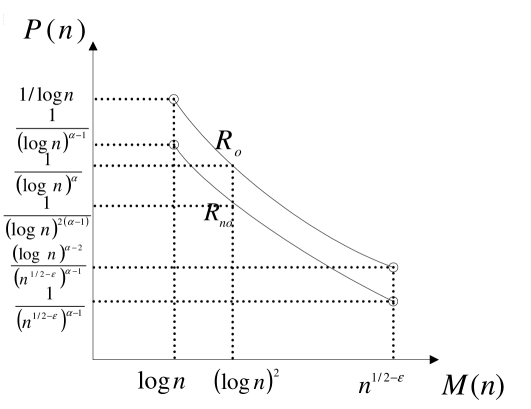
Figure 5: The power scaling with respect to $M(n)$.

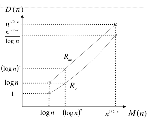
Figure 6: The delay scaling with respect to $M(n)$.

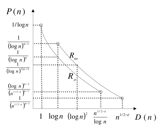
Figure 7: The power–delay trade-off.

Now we show that the opportunistic routing exhibits a net improvement in overall power–delay trade-off over the conventional non-opportunistic routing. Figures 5 and 6 show how the power $P(n)$ and the delay $D(n)$ scale with respect to the number $M(n)$ of simultaneously active S–D pairs, corresponding to the total throughput $T(n)$. $R_{o}$ and $R_{no}$ denote the scaling curves with and without opportunistic routing, respectively. We only take into account the range of $M(n)$ between $\operatorname{log}n$ and $n^{1/2-\epsilon}$ for an arbitrarily small $\epsilon>0$, which is the operating regimes in our work, due to various constraints we assume in the model. Hence, the MUD gain may not be guaranteed if $M(n)$ scales faster than $n^{1/2-\epsilon}$ for a vanishingly small $\epsilon>0$ (e.g., it is shown in [7] that when $M(n)=\Theta(\sqrt{n})$, the benefit of fading cannot be exploited in terms of scaling laws). We observe that $P(n)$ decreases while $D(n)$ increases as we have more active S–D pairs in both schemes. This is because we assume a fixed transmission rate $R>0$ independent of $n$, which implies that for receiver $k(m,l_{m})$ ($l_{m}\in\mathcal{H}_{m}$ and $m\in\{1,\cdots,M(n)\}$), $P_{r}^{k(m,l_{m})}$ and $P_{I}^{k(m,l_{m})}$ need to be $\Omega(1)$ and $O(1)$, respectively, as mentioned earlier. Then, to maintain the interference level $P_{I}^{k(m,l_{m})}$ at $O(1)$ as $M(n)$ increases, more hops per S–D pair are needed, i.e., per-hop distance is reduced. Hence, from the above argument, we may conclude that the power is reduced at the expense of the increased delay, and therefore, there is a fundamental trade-off between the two scaling parameters $P(n)$ and $D(n)$. Furthermore, it is seen that utilizing the opportunistic routing increases the power compared to the non-opportunistic routing case, but it can reduce the delay significantly. Thus, it is not clear whether our opportunistic routing is beneficial or not from Figs. 5 and 6. However, if we plot the power $P(n)$ versus the delay $D(n)$ as in Fig. 7, then it can be clearly seen that opportunistic routing ($R_{o}$) exhibits a better overall power–delay trade-off than that of non-opportunistic routing scheme ($R_{no}$), while providing a logarithmic boost in the scaling law. For example, when opportunistic routing is used, if the delay $D(n)$ is given by $\operatorname{log}n$, then the power $P(n)$ is reduced by $\operatorname{log}n$. In this case, it is further seen from Fig. 6 that the number $M(n)$ of simultaneously supportable S–D pairs is improved by $\operatorname{log}n$, i.e., logarithmic boost on the total throughput $T(n)$. This gain comes from the fact that the received signal power increases due to the MUD gain based on the use of opportunistic routing, which allows more simultaneous transmissions since more interference can be tolerated.

V Conclusion

The scaling behavior of ad hoc networks using opportunistic routing protocol in the presence of fading has been characterized. Specifically, it was shown how the power, delay, and total throughput scale as the number of S–D pairs increases, while maintaining a constant per-node transmission rate. We proved that for the range of simultaneously active S–D pairs between $\operatorname{log}n$ and $n^{1/2-\epsilon}$ for an arbitrarily small $\epsilon>0$, the opportunistic routing exhibits a net improvement in overall power–delay trade-off over the conventional scheme employing non-opportunistic routing, while providing up to a $\operatorname{log}n$ boost in the scaling law due to the MUD gain.

Appendix A appendix

A-A Proof of Lemma 3

There are $8l$ interfering cells in the $l$-th layer of 25-TDMA (refer to Fig. 2). Let $P_{I,(l)}^{k}$ denote the total interference power at a fixed receiver node $k$ from simultaneously transmitting nodes in the $l$-th layer, where $l\in\{1,\cdots,\bar{l}D(n)\}$ for some constant $\bar{l}>0$ independent of $n$. Note that the distance between a receiving node and an interfering node in the $l$-th layer is between $((5l-4)\sqrt{A_{s}(n)},8(5l-4)\sqrt{A_{s}(n)})$. Suppose that the Euclidean distance among the links above is given by $8(5l-4)\sqrt{A_{s}(n)}$, thereby providing a lower bound for $E\left[P_{I,(l)}^{k}\right]$. By Lemma 2, the number of simultaneous transmitters in each cell is given by $\Theta(M(n)/D(n))$ whp. Thus, from (1) and (4), the expectation $E[P_{I}^{(l)}]$ is lower-bounded by

$$E\left[P_{I,(l)}^{k}\right]\!\!\!\!\!\!\! \geq\frac{c_{7}(8l)P(n)/D(n)}{\left(8(5l-4)\sqrt{A_{s}(n)}\right)^{\alpha}}\frac{M(n)}{D(n)}E\left[|g_{ki}|^{2}\right]$$

$$\geq\frac{c_{7}}{8^{\alpha-1}(5l-4)^{\alpha-1}}\frac{P(n)/D(n)}{(\sqrt{A_{s}(n)})^{\alpha}}\frac{M(n)}{D(n)}$$

$$=\frac{c_{8}P(n)M(n)D(n)^{\alpha-2}}{(5l-4)^{\alpha-1}}$$

for any nodes $i$ and $k$, where $c_{7}$ and $c_{8}$ are some positive constants independent of $n$. Similarly by taking $(5l-4)\sqrt{A_{s}(n)}$ for the Euclidean distance between a receiver and simultaneously transmitting nodes in the $l$-th layer, we obtain

$$E\left[P_{I,(l)}^{k}\right]\!\!\!\!\!\!\! \leq\frac{c_{9}P(n)M(n)D(n)^{\alpha-2}}{(5l-4)^{\alpha-1}}$$

for constant $c_{9}>0$ independent of $n$, which results in

$$E\left[P_{I,(l)}^{k}\right]=\Theta\left(\frac{P(n)M(n)D(n)^{\alpha-2}}{(5l-4)^{\alpha-1}}\right).$$

Moreover, let $P_{I,(0)}^{k}$ be the total interference power from other transmitting nodes in the cell including a desired transmitter (see the shaded cell located in the center in Fig. 2). Then as above, we have $E\left[P_{I,(0)}^{k}\right]=\Theta(P(n)M(n)D(n)^{\alpha-2})$, and hence, it follows that $E\left[P_{I}^{k}\right]=\Theta(P(n)M(n)D(n)^{\alpha-2})$ since $\sum_{l}1/(5l-4)^{\alpha-1}$ is bounded by a certain constant for $\alpha>2$.

Now we focus on computing $\Pr\left\{P_{I,(l)}^{k}>(1+\delta_{5})E\left[P_{I,(l)}^{k}\right]\right\}$ by using the Chernoff bound, where $\delta_{5}>0$ is a constant independent of $n$. From the fact that $r_{ki}=\Theta(r_{ki^{\prime}})$ for all transmitting nodes $i$ and $i^{\prime}$ in the same layer and receiving node $k$, we have

$$\Pr\left\{P_{I,(l)}^{k}>(1+\delta_{5})E\left[P_{I,(l)}^{k}\right]\right\}$$

$$=\Pr\left\{\sum_{i\in I_{l}}\frac{|g_{ki}|^{2}}{r_{ki}^{\alpha}}>(1+\delta_{5})E\left[\sum_{i\in I_{l}}\frac{|g_{ki}|^{2}}{r_{ki}^{\alpha}}\right]\right\}$$

$$\leq\Pr\left\{\sum_{i\in I_{l}}\frac{|g_{ki}|^{2}}{\left(5l-4)\sqrt{A_{s}(n)}\right)^{\alpha}}>(1+\delta_{5})E\left[\sum_{i\in I_{l}}\frac{|g_{ki}|^{2}}{r_{ki}^{\alpha}}\right]\right\}$$

$$=\Pr\left\{\sum_{i\in I_{l}}|g_{ki}|^{2}>c_{10}(8l)(1+\delta_{5})\frac{M(n)}{D(n)}\right\}$$ (21)

for constant $c_{10}>0$ independent of $n$. Here, $I_{l}$ is the set of simultaneously interfering nodes in the $l$-th layer. Since the Chernoff bound for the sum of i.i.d. chi-square random variables $|g_{ki}|^{2}$ with two degrees of freedom is given by [35], for a certain constant $0<\epsilon_{1}<\delta_{5}-\operatorname{log}(1+\delta_{5})$, (21) can be upper-bounded by

$$\Pr\left\{P_{I,(l)}^{k}>(1+\delta_{5})E\left[P_{I,(l)}^{k}\right]\right\}\!\!\!\!\!\!\! \leq(1+\delta_{5})^{c_{10}(8l)\frac{M(n)}{D(n)}}\operatorname{exp}\left(-c_{10}(8l)\frac{M(n)}{D(n)}(\delta_{5}-\epsilon_{1})\right)$$

$$\leq(1+\delta_{5})^{8c_{10}\frac{M(n)}{D(n)}}\operatorname{exp}\left(-8c_{10}\frac{M(n)}{D(n)}(\delta_{5}-\epsilon_{1})\right),$$

which tends to zero as $M(n)/D(n)=\omega(1)$. We remark that the event $P_{I,(l)}^{k}>(1+\delta_{5})E\left[P_{I,(l)}^{k}\right]$ for all $l\in\{0,\cdots,\bar{l}D(n)\}$ is a sufficient condition for the event $P_{I}^{k}\leq(1+\delta_{5})E[P_{I}^{k}]$. Thus, by the union bound over all layers (including the cell with a desired transmitter), we have the following inequality:

$$\Pr\bigl{\{}\!\!\!\!\!\!\!\!\! P_{I,(l)}^{k}\leq(1+\delta_{5})E\left[P_{I,(l)}^{k}\right]\text{~{}~{}for all $l\in\{0,\cdots,\bar{l}D(n)\}$}\bigr{\}}$$

$$\geq 1-\sum_{l=0}^{\bar{l}D(n)}\Pr\left\{P_{I,(l)}^{k}>(1+\delta_{5})E\left[P_{I,(l)}^{k}\right]\right\}$$

$$=1-(1+\bar{l}D(n))(1+\delta_{5})^{8c_{10}\frac{M(n)}{D(n)}}$$

$$\quad\cdot\operatorname{exp}\left(-8c_{10}\frac{M(n)}{D(n)}(\delta_{5}-\epsilon_{1})\right),$$

where the first inequality holds since there exist $\bar{l}D(n)$ layers, for some $\bar{l}>0$ independent of $n$. Finally, using the union bound over $n$ nodes in the network yields that the total interference power $P_{I}^{k}$ at receiver node $k$ is given by $O(E[P_{I}^{k}])$ ($=O(P(n)M(n)D(n)^{\alpha-2})$) with probability of at least

$$1-2\bar{l}nD(n)(1+\delta_{5})^{8c_{10}\frac{M(n)}{D(n)}}\operatorname{exp}\left(-8c_{10}\frac{M(n)}{D(n)}(\delta_{5}-\epsilon_{1})\right),$$

which tends to one as $nD(n)\delta_{2}^{-M(n)/D(n)}=o(1)$ for a certain constant

$$1<\delta_{2}<\left(\frac{e^{\delta_{5}-\epsilon_{1}}}{1+\delta_{5}}\right)^{8c_{10}}.$$

This completes the proof of this lemma.

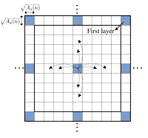
Figure 2: Grouping of interfering cells in the 25-TDMA scheme. The first layer represents the outer eight shaded cells.

References

- [1] P. Gupta and P. R. Kumar, “The capacity of wireless networks,” IEEE Trans. Inf. Theory, vol. 46, pp. 388–404, Mar. 2000.
- [2] D. E. Knuth, “Big Omicron and big Omega and big Theta,” ACM SIGACT News, vol. 8, pp. 18–24, Apr.-June 1976.
- [3] P. Gupta and P. R. Kumar, “Towards an information theory of large networks: an achievable rate region,” IEEE Trans. Inf. Theory, vol. 49, pp. 1877–1894, Aug. 2003.
- [4] O. Dousse, M. Franceschetti, and P. Thiran, “On the throughput scaling of wireless relay networks,” IEEE Trans. Inf. Theory, vol. 52, pp. 2756–2761, June 2006.
- [5] M. Franceschetti, O. Dousse, D. N. C. Tse, and P. Thiran, “Closing the gap in the capacity of wireless networks via percolation theory,” IEEE Trans. Inf. Theory, vol. 53, pp. 1009–1018, Mar. 2007.
- [6] F. Xue, L.-L. Xie, and P. R. Kumar, “The transport capacity of wireless networks over fading channels,” IEEE Trans. Inf. Theory, vol. 51, pp. 834–847, Mar. 2005.
- [7] Y. Nebat, R. L. Cruz, and S. Bhardwaj, “The capacity of wireless networks in nonergodic random fading,” IEEE Trans. Inf. Theory, vol. 55, pp. 2478–2493, June 2009.
- [8] A. El Gamal, J. Mammen, B. Prabhakar, and D. Shah, “Optimal throughput-delay scaling in wireless networks-Part I: The fluid model,” IEEE Trans. Inf. Theory, vol. 52, pp. 2568–2592, June 2006.
- [9] ——, “Optimal throughput-delay scaling in wireless networks-Part II: Constant-size packets,” IEEE Trans. Inf. Theory, vol. 52, pp. 5111–5116, Nov. 2006.
- [10] A. El Gamal and J. Mammen, “Optimal hopping in ad hoc wireless networks,” in Proc. IEEE INFOCOM, Barcelona, Spain, Apr. 2006, pp. 1–10.
- [11] A. Özgür, O. Lévêque, and D. N. C. Tse, “Hierarchical cooperation achieves optimal capacity scaling in ad hoc networks,” IEEE Trans. Inf. Theory, vol. 53, pp. 3549–3572, Oct. 2007.
- [12] U. Niesen, P. Gupta, and D. Shah, “On capacity scaling in arbitrary wireless networks,” IEEE Trans. Inf. Theory, vol. 55, pp. 3959–3982, Sept. 2009.
- [13] A. Jovicic, P. Viswanath, and S. R. Kulkarni, “Upper bounds to transport capacity of wireless networks,” IEEE Trans. Inf. Theory, vol. 50, pp. 2555–2565, Nov. 2004.
- [14] S. Toumpis and A. J. Goldsmith, “Large wireless networks under fading, mobility, and delay constraints,” in Proc. IEEE INFOCOM, Hong Kong, China, Mar. 2004, pp. 609–619.
- [15] R. Knopp and P. Humblet, “Information capacity and power control in single cell multiuser communications,” in Proc. IEEE Int. Conf. Communications (ICC), Seattle, WA, June 1995, pp. 331–335.
- [16] P. Viswanath, D. N. C. Tse, and R. Laroia, “Opportunistic beamforming using dumb antennas,” IEEE Trans. Inf. Theory, vol. 48, pp. 1277–1294, June 2002.
- [17] M. Sharif and B. Hassibi, “On the capacity of MIMO broadcast channels with partial side information,” IEEE Trans. Inf. Theory, vol. 51, pp. 506–522, Feb. 2005.
- [18] S. Cui, A. M. Haimovich, O. Somekh, and H. V. Poor, “Opportunistic relaying in wireless networks,” IEEE Trans. Inf. Theory, vol. 55, pp. 5121–5137, Nov. 2009.
- [19] C. Shen and M. P. Fitz, “Opportunistic spatial orthogonalization and its application to fading cognitive radio networks,” preprint, [Online]. Available: http://arxiv.org/abs/0904.4283.
- [20] R. Gowaikar, B. Hochwald, and B. Hassibi, “Communication over a wireless network with random connections,” IEEE Trans. Inf. Theory, vol. 52, pp. 2857–2871, July 2006.
- [21] M. Ebrahimi, M. A. Maddah-Ali, and A. K. Khandani, “Throughput scaling laws for wireless networks with fading channels,” IEEE Trans. Inf. Theory, vol. 53, pp. 4250–4254, Nov. 2007.
- [22] S.-Y. Chung, “On the transport capacity of wireless ad-hoc networks,” in Proc. Int. Symp. Inform. Theory and its Applications (ISITA), Seoul, Korea, Oct./Nov. 2006, pp. 546–550.
- [23] M. J. Neely and E. Modiano, “Capacity and delay tradeoffs for ad hoc mobile networks,” IEEE Trans. Inf. Theory, vol. 51, pp. 1917–1937, June 2005.
- [24] S. Biswas and R. Morris, “Opportunistic routing in multi-hop wireless networks,” in Proc. ACM HotNets Workshop, Boston, MA, Nov. 2003, pp. 69–74.
- [25] M. Zorzi and R. R. Rao, “Geographic random forwarding (GeRaF) for ad hoc and sensor networks: multihop performance,” IEEE Trans. Mobile Comput., vol. 2, pp. 337–348, Oct.-Dec. 2003.
- [26] R. C. Shah, S. Wietholter, A. Wolisz, and J. M. Rabaey, “Modeling and analysis of opportunistic routing in low traffic scenarios,,” in Proc. The Third International Symposium on Modeling and Optimization in Mobile, Ad Hoc, and Wireless Networks (WiOpt), Trentino, Italy, Apr. 2005, pp. 294–304.
- [27] Z. Zhong and S. Nelakuditi, “On the efficacy of opportunistic routing,” in Proc. IEEE Communications Society Conference on Sensor, Mesh and Ad Hoc Communications and Networks (SECON), San Diego, CA, June 2007, pp. 441–450.
- [28] K. Zeng, W. Lou, and H. Zhai, “On end-to-end throughput of opportunistic routing in multirate and multihop wireless networks,” in Proc. IEEE INFOCOM, Pheonix, AZ, Apr. 2008, pp. 1490–1498.
- [29] A. Bhorkar, M. Naghshvar, T. Javidi, and B. Rao, “An adaptive opportunistic routing scheme for wireless ad-hoc networks,” in Proc. IEEE Int. Symp. Inform. Theory (ISIT), Seoul, Korea, June/July 2009.
- [30] X. Ma, M. T. Sun, G. Zhao, and X. Liu, “Improving geographical routing for wireless networks with an efficient path pruning algorithm,” IEEE Trans. Veh. Technol., vol. 57, pp. 2474–2488, July 2008.
- [31] R. Motwani and P. Raghavan, Randomized Algorithms. Cambridge, U.K.: Cambridge Univ. Press, 1995.
- [32] M. Médard, “The effect upon channel capacity in wireless communications of perfect and imperfect knowledge of the channel,” IEEE Trans. Inf. Theory, vol. 46, pp. 933–946, May 2000.
- [33] S. N. Diggavi and T. M. Cover, “The worst additive noise under a covariance constraint,” IEEE Trans. Inf. Theory, vol. 47, pp. 3072–3081, Nov. 2001.
- [34] S. Weber, J. G. Andrews, and N. Jindal, “The effect of fading, channel inversion, and threshold scheduling on ad hoc networks,” IEEE Trans. Inf. Theory, vol. 53, pp. 4127–4149, Nov. 2007.
- [35] A. Shwartz and A. Weiss, Large Deviations for Performance Analysis. London, U.K.: Champman & Hall, 1995.