QCD Sum Rules for the X(3872) as a mixed molecule-charmoniun state

Abstract

We use QCD sum rules to test the nature of the meson $X(3872)$, assumed to be a mixture between charmonium and exotic molecular $[c\bar{q}][q\bar{c}]$ states with $J^{PC}=1^{++}$. We find that there is only a small range for the values of the mixing angle, $\theta$, that can provide simultaneously good agreement with the experimental value of the mass and the decay width, and this range is $5^{0}\leq\theta\leq 13^{0}$. In this range we get $m_{X}=(3.77\pm 0.18)$ GeV and $\Gamma(X\to J/\psi\pi^{+}\pi^{-})=(9.3\pm 6.9)$ MeV, which are compatible, within the errors, with the experimental values. We, therefore, conclude that the $X(3872)$ is approximately 97% a charmonium state with 3% admixture of $\sim$88% $D^{0}D^{*0}$ molecule and $\sim$12% $D^{+}D^{*-}$ molecule.

I Introduction

Among the new hadronic states discovered in the last few years, the $X(3872)$ is one of the most interesting. It has been first observed by the Belle collaboration in the decay $B^{+}\!\rightarrow\!X(3872)K^{+}\rightarrow\!J/\psi\pi^{+}\pi^{-}K^{+}$ belle1 . This observation was later confirmed by CDF, D0 and BaBar Xexpts . The current world average mass is $m_{X}=(3871.4\pm 0.6)\mbox{ MeV}$ which is at the threshold for the production of the charmed meson pair ${D^{0}}{\bar{D}}^{0\ast}$. This state is extremely narrow, with a width smaller than 2.3 MeV at 90% confiedence level. Both Belle and Babar collaborations reported the radiative decay mode $X(3872)\to\gamma J/\psi$ belleE ; babar2 , which determines $C=+$. Further studies from Belle and CDF that combine angular information and kinematic properties of the $\pi^{+}\pi^{-}$ pair, strongly favor the quantum numbers $J^{PC}=1^{++}$ or $2^{-+}$ belleE ; cdf2 ; cdf3 .

In constituent quark models bg the masses of the possible charmonium states with $J^{PC}=1^{++}$ quantum numbers are: $2~{}^{3}P_{1}(3990)$ and $3~{}^{3}P_{1}(4290)$, which are much bigger than the observed mass. In view of this large mass discrepancy the attempts to understand the $X$ meson as a conventional quark-antiquark states were abandoned. The next possibility explored was to treat this state as a multiquark state, composed by $c$, $\overline{c}$ and a light quark antiquark pair. Another experimental finding in favor of this conjecture is the the fact that the decay rates of the processes $X(3872)\to J/\psi\,\pi^{+}\pi^{-}\pi^{0}$ and $X(3872)\rightarrow\!J/\psi\pi^{+}\pi^{-}$ are comparable belleE :

$${X\to J/\psi\,\pi^{+}\pi^{-}\pi^{0}\over X\to\!J/\psi\pi^{+}\pi^{-}}=1.0\pm 0.4\pm 0.3.$$ (1)

This ratio indicates a strong isospin and G parity violation, which is incompatible with a $c\bar{c}$ structure for $X(3872)$.

In a multiquark approach we can avoid the isospin violation problem. The next natural question is: is the $X$ made by four quarks in a bag or by a meson-meson molecule?

The observation of the above mentioned decays, plus the coincidence between the $X$ mass and the $D^{*0}D^{0}$ threshold: $M(D^{*0}D^{0})=(3871.81\pm 0.36)\mbox{ MeV}$ cleo , inspired the proposal that the $X(3872)$ could be a molecular $(D^{*0}\bar{D}^{0}-\bar{D}^{*0}D^{0})$ bound state with small binding energy close ; swanson . The $D^{*0}\bar{D}^{0}$ molecule is not an isospin eigenstate and the rate in Eq.(1) could be explained in a very natural way in this model.

Maiani and collaborators maiani suggested that $X(3872)$ is a tetraquark. They have considered diquark-antidiquark states with $J^{PC}=1^{++}$ and symmetric spin distribution:

$$X_{q}=[cq]_{S=1}[\bar{c}\bar{q}]_{S=0}+[cq]_{S=0}[\bar{c}\bar{q}]_{S=1}.$$ (2)

The isospin states with $I=0,~{}1$ are given by:

$$X(I=0)={X_{u}+X_{d}\over\sqrt{2}},\;\;\;\;X(I=1)={X_{u}-X_{d}\over\sqrt{2}}.$$ (3)

In maiani the authors argue that the physical states are closer to mass eigenstates and are no longer isospin eigenstates. The most general states are then:

$$X_{l}=\cos{\theta}X_{u}+\sin{\theta}X_{d},\;\;\;\;X_{h}=\cos{\theta}X_{d}-\sin{\theta}X_{u},$$ (4)

and both can decay into $2\pi$ and $3\pi$. Imposing the rate in Eq.(1), they obtain $\theta\sim 20^{0}$. They also argue that if $X_{l}$ dominates $B^{+}$ decays, then $X_{h}$ dominates the $B^{0}$ decays and vice-versa. Therefore, the $X$ particle in $B^{+}$ and $B^{0}$ decays would be different with maiani ; polosa $M(X_{h})-M(X_{l})=(8\pm 3)\mbox{ MeV}$. There are indeed reports from Belle belleB0 and Babar babarB0 Collaborations on the observation of the $B^{0}\to K^{0}~{}X$ decay. However, these reports (not completely consistent with each other) point to a mass difference much smaller than the predicited $\simeq 8\mbox{ MeV}$.

All the conclusions in ref. maiani were obtained in the context of a quark model. Given the uncertainties inherent to hadron spectroscopy, it is interesting to confront these theoretical results with QCD sum rules (QCDSR) calculations. This was partly done in x3872 where, using the same tetraquark structure proposed in ref. maiani , the mass difference $M(X_{h})-M(X_{l})$ was computed and found to be in agreement with the BaBar measurement ($M(X_{h})-M(X_{l})=(3.3\pm 0.7)\mbox{ MeV}$). The same calculation x3872 has obtained $m_{X}=(3.92\pm 0.13)\mbox{ GeV}$. In QCDSR we can also use a current with the features of the mesonic molecule of the type $(D^{*0}\bar{D}^{0}-\bar{D}^{*0}D^{0})$. With such a current the calculation reported in lnw obtained the mass $m_{X}=(3.87\pm 0.07)\mbox{ GeV}$ in a better agreement with the experimental mass. Therefore, from a QCDSR point of view, the $X(3872)$ seems to be better described with a $D^{*}D$ molecular current than with a diquark-antidiquark current. We feel though that the subject deserves further investigation.

In this work we use again the QCDSR approach to the $X$ structure including a new possibility: the mixing between two and four-quark states. This will be implemented folowing the prescription suggested in oka24 for the light sector. The mixing is done at the level of the currents and will be extended to the charm sector. In a different context (not in QCDSR), a similar mixing was suggested already some time ago by Suzuki suzuki . Physically, this corresponds to a fluctuation of the $c\overline{c}$ state where a gluon is emitted and subsequently splits into a light quark-antiquark pair, which lives for some time and behaves like a molecule-like state. As it will be seen, in order to be consistent with $X$ decay data, we must consider a second mixing between: $(c\overline{c})\,+\,(D^{*0}\bar{D}^{0}-\bar{D}^{*0}D^{0})$ and $(c\overline{c})\,+\,(D^{*+}\bar{D}^{-}-\bar{D}^{*-}D^{+})$.

With all these ingredients we perform a calculation of the mass of the $X(3872)$ and its decay width into $2\pi$ and $3\pi$.

II The mixed two-quark / four quark operator

There are some experimental data on the $X(3872)$ meson that seem to indicate the existence of a $c\bar{c}$ component in its structure. In ref. suzuki it was shown that, because of the very loose binding of the molecule, the production rates of a pure $X(3872)$ molecule should be at least one order of magnitude smaller than what is seen experimentally. Also, the recent observation, reported by BaBar babar09 , of the decay $X(3872)\to\psi(2S)\gamma$ at a rate:

$${{\cal B}(X\to\psi(2S)\,\gamma)\over{\cal B}(X\to\psi\gamma)}=3.4\pm 1.4,$$ (5)

is much bigger than the molecular prediction  swan1 :

$${\Gamma(X\to\psi(2S)\,\gamma)\over\Gamma(X\to\psi\gamma)}\sim 4\times 10^{-3}.$$ (6)

While this difference could be interpreted as a strong point against the molecular model and as a point in favor of a conventional charmonium interpretation, it can also be interpreted as an indication that there is a significant mixing of the $c\bar{c}$ component with the $D^{0}\bar{D}^{*0}$ molecule. Similar conclusion was also reached in refs. li1 ; li2 . Therefore, we will follow ref. oka24 and consider a mixed charmonium-molecular current to study the $X(3872)$ in the QCD Sum Rule framework.

For the charmonium part we use the conventional axial current:

$$j^{\prime(2)}_{\mu}(x)=\bar{c}_{a}(x)\gamma_{\mu}\gamma_{5}c_{a}(x).$$ (7)

The $D^{0}$ $D^{*0}$ molecule is interpolated by liuliu ; dong ; stancu :

$$j^{(4u)}_{\mu}(x) = {1\over\sqrt{2}}\bigg{[}\left(\bar{u}_{a}(x)\gamma_{5}c_{a}(x)\bar{c}_{b}(x)\gamma_{\mu}u_{b}(x)\right)$$ (8)

$$- \left(\bar{u}_{a}(x)\gamma_{\mu}c_{a}(x)\bar{c}_{b}(x)\gamma_{5}u_{b}(x)\right)\bigg{]},$$

As in ref. oka24 we define the normalized two-quark current as

$$j^{(2u)}_{\mu}={1\over 6\sqrt{2}}\langle\bar{u}u\rangle j^{\prime(2)}_{\mu},$$ (9)

and from these two currents we build the following mixed charmonium-molecular current for the $X(3872)$:

$$J_{\mu}^{u}(x)=\sin(\theta)j^{(4u)}_{\mu}(x)+\cos(\theta)j^{(2u)}_{\mu}(x).$$ (10)

III The two point correlator

The QCD sum rules svz ; rry ; SNB are constructed from the two-point correlation function

$$\Pi_{\mu\nu}(q)=i\int d^{4}x~{}e^{iq.x}\langle 0|T[J_{\mu}^{u}(x)J_{\nu}^{u\dagger}(0)]|0\rangle=$$

$$=-\Pi_{1}(q^{2})\left(g_{\mu\nu}-{q_{\mu}q_{\nu}\over q^{2}}\right)+\Pi_{0}(q^{2}){q_{\mu}q_{\nu}\over q^{2}}.$$ (11)

As the axial vector current is not conserved, the two functions, $\Pi_{1}$ and $\Pi_{0}$, appearing in Eq. (11) are independent and have respectively the quantum numbers of the spin 1 and 0 mesons.

The sum rules approach is based on the principle of duality. It consists in the assumption that the correlation function may be described at both quark and hadron levels. At the hadronic level (the phenomenological side) the correlation function is calculated introducing hadron characteristics such as masses and coupling constants. At the quark level, the correlation function is written in in terms of quark and gluon fields and a Wilson’s operator product expansion (OPE) is used to deal with the complex structure of the QCD vacuum.

The phenomenological side is treated by first parametrizing the coupling of the axial vector meson $1^{++}$, $X$, to the current, $J_{\mu}^{u}$, in Eq. (10) in terms of the meson-current coupling parameter $\lambda^{u}$:

$$\langle 0|J_{\mu}^{u}|X\rangle=\lambda^{u}\epsilon_{\mu}~{}.$$ (12)

Then, by inserting intermediate states for the meson $X$, we can write the phenomenological side of Eq. (11) as

$$\Pi_{\mu\nu}^{phen}(q)={(\lambda^{u})^{2}\over m_{X}^{2}-q^{2}}\left(-g_{\mu\nu}+{q_{\mu}q_{\nu}\over m_{X}^{2}}\right)+\cdots\;,$$ (13)

where the Lorentz structure projects out the $1^{++}$ state. The dots denote higher mass axial-vector resonances. This ressonances will be dealt with through the introduction of a continuum threshold parameter $s_{0}$.

In ref. 2hr it was argued that a single pole ansatz can be problematic in the case of a multiquark state, and that the two-hadron reducible (2HR) contribution (or $S$-wave $D\bar{D}^{*}$ contribution, in the present case) should also be considered in the phenomenological side. However, in ref. 2hr2 it was shown that the 2HR contribution is very small. The reason for this is the following. The 2HR contribution, in our case, can be written as 2hr2 :

$$\Pi_{\mu\nu}^{2HR}(q) = i(\lambda_{DD^{*}})^{2}\int~{}{d^{4}p\over(2\pi)^{4}}\bigg{(}{-g_{\mu\nu}+p_{\mu}p_{\nu}/m_{D^{*}}^{2}\over p^{2}-m_{D^{*}}^{2}}$$ (14)

$$\times {1\over(p-q)^{2}-m_{D}^{2}}\bigg{)},$$

where

$$\langle 0|j_{\mu}^{(4u)}|DD^{*}(p)\rangle=\lambda_{DD^{*}}\varepsilon_{\mu}(p).$$ (15)

Following ref. 2hr2 the current two-meson coupling: $\lambda_{DD^{*}}$, can be written in terms of the $D$ meson decay constant, $f_{D}$, and the coupling of the $D^{*}$ meson with a 4-quark current. This last quantity should be very small, because the properties of the $D^{*}$ meson, both in spectroscopy and in scattering, are very well understood if it is an ordinary quark-antiquark state. Therefore, the parameter $\lambda_{DD^{*}}$, should be very small, as in the case of the pentaquark 2hr2 , and the 2HR contribution can be safely neglected.

In the OPE side we work up to dimension 8 at the leading order in $\alpha_{s}$. The light quark propagators are calculated in coordinate-space and then Fourier transformed to the momentum space. The charm quark part is calculated directly into the momentum space, with finite $m_{c}$, and combined with the light part. The correlator in Eq. (11) can be written as:

$$\Pi_{\mu\nu}(q) = \left({\langle\bar{u}u\rangle\over 6\sqrt{2}}\right)^{2}\cos^{2}(\theta)\,\Pi^{(2,2)}_{\mu\nu}(q)+$$ (16)

$$+ {\langle\bar{u}u\rangle\over 6\sqrt{2}}\left(\sin(2\theta)\right)\,\Pi^{(2,4)}_{\mu\nu}(q)+$$

$$+ \sin^{2}(\theta)\,\Pi^{(4,4)}_{\mu\nu}(q),$$

with:

$$\Pi^{(i,j)}_{\mu\nu}(q)=i\int d^{4}x~{}e^{iq.x}\langle 0|T[j^{(i)}_{\mu}(x)j^{(j)\dagger}_{\nu}(0)]|0\rangle.$$ (17)

After making a Borel transform of both sides, and transferring the continuum contribution to the OPE side, the sum rule for the axial vector meson up to dimension-eight condensates can be written as:

$$(\lambda^{u})^{2}e^{-m_{X}^{2}/M^{2}}=$$

$$=\left({\langle\bar{u}u\rangle\over 6\sqrt{2}}\right)^{2}\cos^{2}(\theta)\,\Pi^{(2,2)}_{1}(M^{2})+$$

$$+{\langle\bar{u}u\rangle\over 6\sqrt{2}}\left(\sin(2\theta)\right)\,\Pi^{(2,4)}_{1}(M^{2})+$$

$$+\,\sin^{2}(\theta)\,\Pi^{(4,4)}_{1}(M^{2}),$$ (18)

where:

$$\Pi^{(2,2)}_{1}(M^{2})=\!\!\int_{4m_{c}^{2}}^{s_{0}}\!\!\!\!ds~{}e^{-s/M^{2}}\rho_{pert}^{(22)}(s)\;+\Pi^{(22)}_{\langle G^{2}\rangle}(M^{2}),\;$$ (19)

$$\Pi^{(2,4)}_{1}(M^{2})=\!\!\int_{4m_{c}^{2}}^{s_{0}}\!\!\!\!ds~{}e^{-s/M^{2}}\rho^{(24)}_{\langle\bar{u}u\rangle}(s)\;+\Pi^{(24)}_{\langle\bar{u}Gu\rangle}(M^{2}),\;$$ (20)

$$\Pi^{(4,4)}_{1}(M^{2}) = \!\!\int_{4m_{c}^{2}}^{s_{0}}\!\!\!\!ds~{}e^{-s/M^{2}}\Bigg{[}\rho_{pert}^{(44)}(s)+\rho^{(44)}_{\langle\bar{u}u\rangle}(s)+$$ (21)

$$+ \rho^{(44)}_{\langle\bar{u}u\rangle^{2}}(s)+\rho^{(44)}_{\langle G^{2}\rangle}(s)+\rho^{(44)}_{\langle\bar{u}Gu\rangle}(s)\Bigg{]}+$$

$$+ \Pi^{(44)}_{\langle\bar{u}u\rangle\langle\bar{u}Gu\rangle}(M^{2}),\;$$

and

$$\rho_{pert}^{(22)}(s)=\frac{s}{4\pi^{2}}\left(1-\frac{4m_{c}^{2}}{s}\right)^{\frac{3}{2}},\;$$ (22)

$$\Pi^{(22)}_{\langle G^{2}\rangle}(M^{2}) =-\frac{\langle g^{2}G^{2}\rangle}{3\cdot 2^{5}\pi^{2}}\int_{0}^{1}d\alpha\Bigg{[}\frac{2\alpha(1-\alpha)M^{2}+m_{c}^{2}}{\alpha(1-\alpha)M^{2}}+$$

$$+2m_{c}^{2}\frac{(2\alpha-1)m_{c}^{2}+\alpha(\alpha^{2}-1)M^{2}}{M^{4}\alpha^{3}(\alpha-1)}\Bigg{]}e^{-\frac{m_{c}^{2}}{\alpha(1-\alpha)M^{2}}},\;$$

$$\rho^{(24)}_{\langle\bar{u}u\rangle}(s)=-\frac{\langle\bar{u}u\rangle}{6\sqrt{2}}\rho_{pert}^{(22)}(s),\;$$ (24)

$$\Pi^{(24)}_{\langle G^{2}\rangle}(M^{2})=-\frac{\langle\bar{u}u\rangle}{6\sqrt{2}}\Pi^{(22)}_{\langle G^{2}\rangle}(M^{2})$$ (25)

$$\Pi^{(24)}_{\langle\bar{u}Gu\rangle}(M^{2}) =\frac{5\langle\bar{q}g_{s}\sigma\cdot Gq\rangle}{3\cdot 2^{6}\sqrt{2}\pi^{2}}\int_{0}^{1}d\alpha\,\frac{m_{c}^{2}}{1-\alpha}\,e^{-\frac{m_{c}^{2}}{\alpha(1-\alpha)M^{2}}},\;$$ (26)

$$\rho^{(44)}_{pert}(s) =\frac{3}{2^{12}\pi^{6}}\int_{\alpha_{min}}^{\alpha_{max}}d\alpha\int_{\beta_{min}}^{\beta_{max}}d\beta\,\frac{1-\left(\alpha+\beta\right)^{2}}{\alpha^{3}\beta^{3}}K^{4}(\alpha,\beta),\;$$

$$\rho^{(44)}_{\langle\bar{u}u\rangle}(s) =-\frac{3m_{c}\langle\bar{u}u\rangle}{2^{7}\pi^{4}}\int_{\alpha_{min}}^{\alpha_{max}}\!d\alpha\int_{\beta_{min}}^{\beta_{max}}\!d\beta\frac{(1+\alpha+\beta)}{\alpha\beta^{2}}\!K^{2}(\alpha,\beta),\;$$

$$\rho^{(44)}_{\langle\bar{u}u\rangle^{2}}(s)=\frac{m_{c}^{2}}{2^{4}\pi^{2}}\langle\bar{u}u\rangle^{2}\sqrt{1-\frac{4m_{c}^{2}}{s}},\;$$ (29)

$$\rho^{(44)}_{\langle G^{2}\rangle}(s) =\frac{\langle g^{2}G^{2}\rangle}{2^{11}\pi^{6}}\int_{\alpha_{min}}^{\alpha_{max}}d\alpha\int_{\beta_{min}}^{\beta_{max}}d\beta\Bigg{[}m_{c}^{2}\frac{(1-(\alpha+\beta)^{2})}{\alpha^{3}}$$

$$-\frac{1-2\alpha-2\beta}{\alpha\beta^{2}}K(\alpha,\beta)\Bigg{]}K(\alpha,\beta),\;$$

$$\rho^{(44)}_{\langle\bar{u}Gu\rangle}(s) =-\frac{3m_{c}}{2^{8}\pi^{4}}\langle\bar{u}g\sigma\cdot Gu\rangle\int_{\alpha_{min}}^{\alpha_{max}}d\alpha\Bigg{[}\frac{2(m_{c}^{2}-\alpha(1-\alpha)s)}{1-\alpha}$$ (31)

$$-\int_{\beta_{min}}^{\beta_{max}}d\beta\,\Bigg{(}1-2\frac{\alpha+\beta}{\beta}\Bigg{)}\frac{K(\alpha,\beta)}{\beta}\Bigg{]},\;$$

$$\Pi^{(44)}_{\langle\bar{u}u\rangle\langle\bar{u}Gu\rangle}(M^{2}) =-\frac{m_{c}^{2}\langle\bar{u}u\rangle\langle\bar{u}g_{s}\sigma\cdot Gu\rangle}{2^{5}\pi^{2}}\int_{0}^{1}d\alpha\Bigg{[}\frac{\alpha(1-\alpha)M^{2}+m_{c}^{2}}{\alpha(1-\alpha)M^{2}}$$ (32)

$$-\frac{1}{1-\alpha}\Bigg{]}e^{-\frac{m_{c}^{2}}{\alpha(1-\alpha)M^{2}}}.\;$$

The integration limits are:

$$\alpha_{min}=\frac{1-\sqrt{1-\frac{4m_{c}^{2}}{s}}}{2},\qquad\alpha_{max}=\frac{1+\sqrt{1-\frac{4m_{c}^{2}}{s}}}{2}$$

$$\beta_{min}=\frac{\alpha}{\alpha\frac{q^{2}}{m_{c}^{2}}-1},\qquad\beta_{max}=1-\alpha$$

and we define $K(\alpha,\beta)\equiv(\alpha+\beta)m_{c}^{2}-\alpha\beta q^{2}$.

By taking the derivative of Eq. (18) with respect to $1/M^{2}$ and dividing the result by Eq. (18) we can obtain the mass of $m_{X}$ without worrying about the value of the meson-current coupling $\lambda^{u}$. The expression thus obtained is analised numerically using the following values for quark masses and QCD condensates x3872 ; narpdg :

$$m_{c}(m_{c})=(1.23\pm 0.05)\,\mbox{ GeV},$$

$$\langle\bar{u}u\rangle\,-(0.23\pm 0.03)^{3}\,\mbox{ GeV}^{3},$$

$$\langle\bar{u}g\sigma.Gu\rangle=m_{0}^{2}\langle\bar{u}u\rangle,$$

$$m_{0}^{2}=0.8\,\mbox{ GeV}^{2},$$

$$\langle g^{2}G^{2}\rangle=0.88~{}\mbox{ GeV}^{4}.$$ (33)

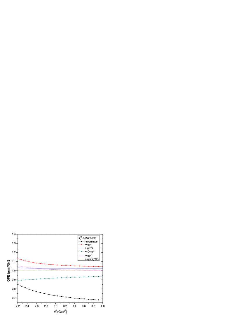
Figure 1: Relative contributions of the terms in eqs. (22) to (32) grouped by condensate dimensions. We start with the perturbative contribution and each subsequent line represents the addition of one extra condensate dimension in the expansion.

In Fig. 1 we show the contributions of the terms in Eqs. (22) to (32) grouped by condensate dimensions divided by the RHS of Eq. (18). We have used $s_{0}^{1/2}=4.4$ GeV and $\theta=9^{\circ}$, but the situation does not change much for other choices of these parameters. It is clear that the OPE is converging for values of $M^{2}\geq 2.6$ GeV² and we will limit our analysis to that region.

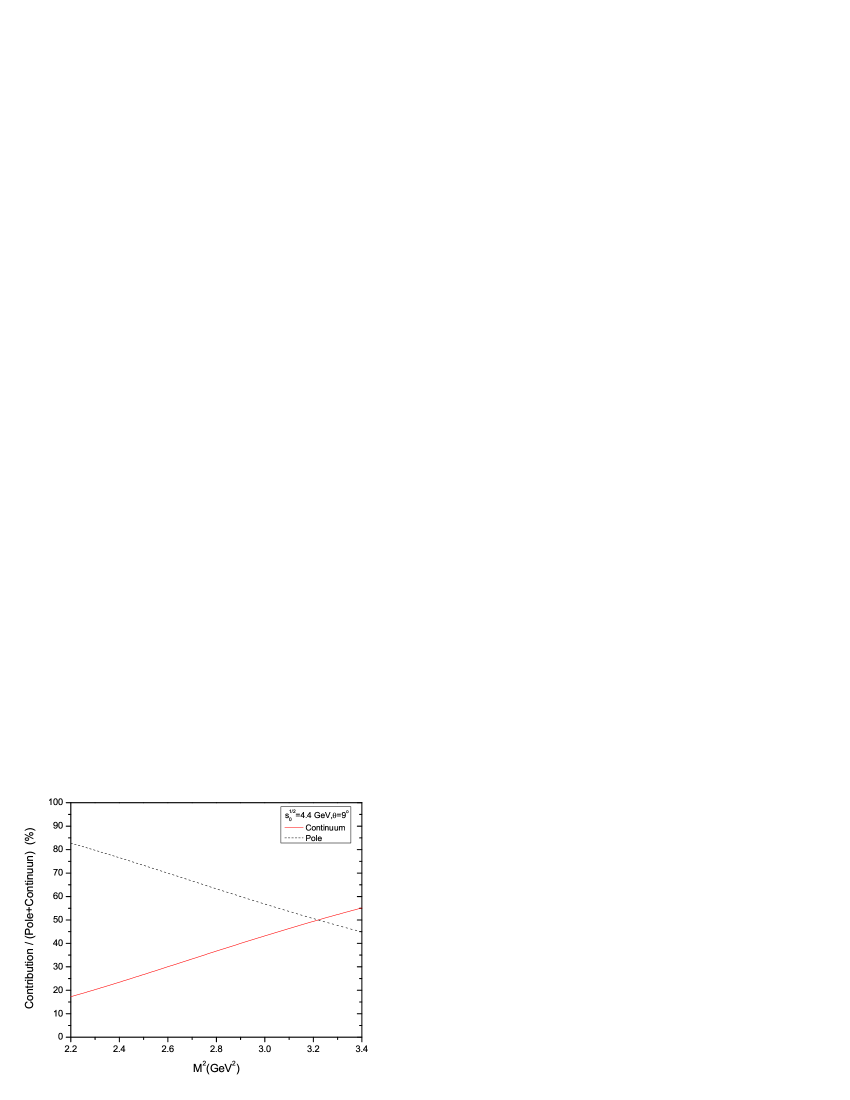
Figure 2: The dashed line shows the relative pole contribution (the pole contribution divided by the total, pole plus continuum, contribution) and the solid line shows the relative continuum contribution.

The upper limit to the value of $M^{2}$ comes by imposing that the QCD pole contribution should be bigger than the continuun contribution. The maximum value of $M^{2}$ that satisfies this condition depends on the value of $s_{0}$, being more restrictive for smaller $s_{0}$. In Fig. 2 we show a comparison between the pole and continuun contributions for the smaller $s_{0}$ we will be considering ($s_{0}^{1/2}=4.4$) and $\theta=9^{\circ}$. The condition obtained from Fig. 2 is $M^{2}\leq 3.2$ GeV², but in this case, the dependence on the choice of $\theta$ is very strong. Taking into account the variation of $\theta$ we have determined that, for $5^{\circ}\leq\theta\leq 13^{\circ}$, the QCDSR are valid in the following region:

$$2.6\mbox{ GeV}^{2}\leq M^{2}\leq 3.0\mbox{ GeV}^{2}$$ (34)

In Fig. 3, we show the $X$ meson mass in this region. We see that the results are reasonably stable as a function of $M^{2}$.

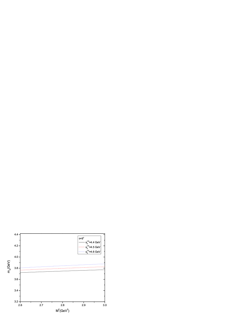
Figure 3: The $X$ meson mass as a function of the sum rule parameter ($M^{2}$) in the region of eq. (34) for different values of the continuum threshold: $s_{0}^{1/2}=4.4$ GeV (solid line), $s_{0}^{1/2}=4.5$ GeV (dashed line) and $s_{0}^{1/2}=4.6$ GeV (dotted line).

From Fig. 3 we obtain $m_{X}=(3.80\pm 0.08)\mbox{ GeV}$ where the error includes the variation of both $s_{0}$ and $M^{2}$. If we also take into account the variation of $\theta$ in the region $5^{\circ}\leq\theta\leq 13^{\circ}$ we get:

$$m_{X}=(3.77\pm 0.18)\mbox{ GeV},$$ (35)

which is in a good agreement with the experimental value. The value obtained for the mass grows with the value of the mixing angle $\theta$, but for $\theta\geq 30^{\circ}$ it reaches a stable value being completely determined by the molecular part of the current.

From Eq. (18) we can also obtain $\lambda^{u}$ by fixing $m_{X}$ equal to the experimental value ($m_{X}=3.87\mbox{ GeV}$). Using the same region in $\theta$, $s_{0}$ and $M^{2}$ that we have used in the mass analysis we obtain:

$$\lambda^{u}=(3.6\pm 0.9).10^{-3}\mbox{ GeV}^{5}.$$ (36)

IV Decay of the X(3872) and the three point correlator

As discussed in Sec. I, one of the most intriguing facts about the meson $X(3872)$ is the observation, reported by the BELLE collaboration belleE , that the $X$ decays into $J/\psi\,\pi^{+}\pi^{-}\pi^{0}$, with a strength that is compatible to that of the $J/\psi\pi^{+}\pi^{-}$ mode, as given by Eq .(1). This decay suggests an appreciable transition rate to $J/\psi\,\omega$ and establishes strong isospin violating effects. It still does not completely exclude a $c\bar{c}$ interpretation for $X$ since the origin of the isospin and G parity non-conservation in Eq. (1) could be of dynamical origin due to $\rho^{0}-\omega$ mixing tera . However, the observation of the ratio in Eq. (1) is an important point in favor of the molecular picture proposed by Swanson swan1 . In this molecular picture the $X(3872)$ is mainly a $D^{0}\bar{D}^{*0}$ molecule with a small but important admixture of $\rho J/\psi$ and $\omega J/\psi$ components.

It is important to notice that, although a $D^{0}\bar{D}^{*0}$ molecule is not an isospin eingenstate, the ratio in Eq. (1) can not be reproduced by a pure $D^{0}\bar{D}^{*0}$ molecule. This can be seen through the observation that the decay width for the decay $X\to J/\psi V\to J/\psi F$ where $F=\pi^{+}\pi^{-}(\pi^{+}\pi^{-}\pi^{0})$ for $V=\rho(\omega)$ is given by maiani ; decayx

$${d\Gamma\over ds}(X\to J/\psi f)={1\over 8\pi m_{X}^{2}}|{\cal{M}}|^{2}B_{V\to F}$$ (37)

$$\times {\Gamma_{V}m_{V}\over\pi}{p(s)\over(s-m_{V}^{2})^{2}+(m_{V}\Gamma_{V})^{2}},$$

where

$$p(s)={\sqrt{\lambda(m_{X}^{2},m_{\psi}^{2},s)}\over 2m_{X}},$$ (38)

with $\lambda(a,b,c)=a^{2}+b^{2}+c^{2}-2ab-2ac-2bc$. The invariant amplitude squared is given by:

$$|{\cal M}|^{2}=g_{X\psi V}^{2}f(m_{X},m_{\psi},s),$$ (39)

where $g_{X\psi V}$ is the coupling constant in the vertex $XJ/\psi V$ and

$$f(m_{X},m_{\psi},s)={1\over 3}\left(4m_{X}^{2}-{m_{\psi}^{2}+s\over 2}+{(m_{X}^{2}-m_{\psi}^{2})^{2}\over 2s}\right.$$ (40)

$$+ \left.{(m_{X}^{2}-s)^{2}\over 2m_{\psi}^{2}}\right){m_{X}^{2}-m_{\psi}^{2}+s\over 2m_{X}^{2}}.$$

Therefore, the ratio in Eq. (1) is given by:

$${\Gamma(X\to J/\psi\,\pi^{+}\pi^{-}\pi^{0})\over\Gamma(X\to J/\psi\,\pi^{+}\pi^{-})}={g_{X\psi\omega}^{2}m_{\omega}\Gamma_{\omega}B_{\omega\to\pi\pi\pi}I_{\omega}\over g_{X\psi\rho}^{2}m_{\rho}\Gamma_{\rho}B_{\rho\to\pi\pi}I_{\rho}},$$ (41)

where

$$I_{V} = \int_{(nm_{\pi})^{2}}^{(m_{X}-m_{\psi})^{2}}ds\bigg{(}f(m_{X},m_{\psi},s)$$ (42)

$$\times {p(s)\over(s-m_{V}^{2})^{2}+(m_{V}\Gamma_{V})^{2}}\bigg{)}.$$

Using $B_{\omega\to\pi\pi\pi}=0.89$, $\Gamma_{\omega}=8.49\mbox{ GeV}$, $m_{\omega}=782.6\mbox{ MeV}$, $B_{\rho\to\pi\pi}=1$, $\Gamma_{\rho}=149.4\mbox{ GeV}$ and $m_{\rho}=775.5\mbox{ MeV}$ we get

$${\Gamma(X\to J/\psi\,\pi^{+}\pi^{-}\pi^{0})\over\Gamma(X\to J/\psi\,\pi^{+}\pi^{-})}=0.118\left({g_{X\psi\omega}\over g_{X\psi\rho}}\right)^{2}.$$ (43)

The couplings, $g_{X\psi V}$, can be evaluated through a QCDSR calculation for the vertex, $X(3872)J/\psi V$, that centers in the three-point function given by

$$\Pi_{\mu\nu\alpha}(p,p^{\prime},q)=\int d^{4}xd^{4}y~{}e^{ip^{\prime}.x}~{}e^{iq.y}\Pi_{\mu\nu\alpha}(x,y),$$ (44)

with

$$\Pi_{\mu\nu\alpha}(x,y)=\langle 0|T[j_{\mu}^{\psi}(x)j_{\nu}^{V}(y){j_{\alpha}^{X}}^{\dagger}(0)]|0\rangle,$$ (45)

where $p=p^{\prime}+q$ and the interpolating fields are given by:

$$j_{\mu}^{\psi}=\bar{c}_{a}\gamma_{\mu}c_{a},$$ (46)

$$j_{\nu}^{V}={N_{V}\over 2}(\bar{u}_{a}\gamma_{\nu}u_{a}+(-1)^{I_{V}}\bar{d}_{a}\gamma_{\nu}d_{a}),$$ (47)

with $N_{\rho}=1$, $I_{\rho}=1$, $N_{\omega}=1/3$ and $I_{\omega}=0$. If $X(3872)$ is a pure $D^{0}\bar{D}^{*0}$ molecule, $j_{\alpha}^{X}$ is given by Eq. (8). In this case the only difference in the OPE side of the sum rule is the factor $N_{V}$ and, therefore, regardless the approximations made in the OPE side and the number of terms considered in the sum rule one has

$$\Pi_{\mu\nu\alpha}^{V}(p,p^{\prime},q)=N_{V}\Pi_{\mu\nu\alpha}^{OPE}(p,p^{\prime},q).$$ (48)

To evaluate the phenomenological side of the sum rule we insert, in Eq.(45), intermediate states for $X$, $J/\psi$ and $V$. We get decayx :

$$\Pi_{\mu\nu\alpha}^{(phen)}(p,p^{\prime},q)={i\lambda_{X}m_{\psi}f_{\psi}m_{V}f_{V}~{}g_{X\psi V}\over(p^{2}-m_{X}^{2})({p^{\prime}}^{2}-m_{\psi}^{2})(q^{2}-m_{V}^{2})}$$ (49)

$$\times \bigg{(}-\epsilon^{\alpha\mu\nu\sigma}(p^{\prime}_{\sigma}+q_{\sigma})-\epsilon^{\alpha\mu\sigma\gamma}{p^{\prime}_{\sigma}q_{\gamma}q_{\nu}\over m_{V}^{2}}$$

$$- \epsilon^{\alpha\nu\sigma\gamma}{p^{\prime}_{\sigma}q_{\gamma}p^{\prime}_{\mu}\over m_{\psi}^{2}}\bigg{)}.$$

Therefore, for a given structure the sum rule is given by:

$${i\lambda_{X}m_{\psi}f_{\psi}m_{V}f_{V}~{}g_{X\psi V}\over(p^{2}-m_{X}^{2})({p^{\prime}}^{2}-m_{\psi}^{2})(q^{2}-m_{V}^{2})}=N_{V}\Pi^{OPE}(p,p^{\prime},q),$$ (50)

from where, considering $m_{\rho}\simeq m_{\omega}$ one gets:

$${g_{X\psi\omega}f_{\omega}\over g_{X\psi\rho}f_{\rho}}={N_{\omega}\over N_{\rho}}={1\over 3}.$$ (51)

Using $f_{\rho}=157\mbox{ MeV}$ and $f_{\omega}=46\mbox{ MeV}$ we obtain

$${g_{X\psi\omega}\over g_{X\psi\rho}}=1.14,$$ (52)

and using this result in Eq. (43) we finally get

$${\Gamma(X\to J/\psi\,\pi^{+}\pi^{-}\pi^{0})\over\Gamma(X\to J/\psi\,\pi^{+}\pi^{-})}\simeq 0.15.$$ (53)

It is very important to notice that this is a very general result that does not depend on any approximation in the QCDSR. This result shows that the admixture of $\rho J/\psi$ and $\omega J/\psi$ components in the molecular model of ref.swan1 is indeed very important to reproduce the data in Eq. (1). It is also important to notice that, in a QCDSR calculation of the decay rate $X\to J/\psi V$, the $c\bar{c}$ admixture in the $D^{0}\bar{D}^{*0}$ molecule, as given by Eq. (10), does not solve the problem of geting the ratio in Eq.(1). This can be seen by using, in Eq. (45), ${j_{\alpha}^{X}}=J_{\alpha}^{u}$, with $J_{\alpha}^{u}$ given by Eq. (10). One gets:

$$\Pi_{\mu\nu\alpha}(x,y) = {\langle\bar{u}u\rangle\over 2\sqrt{6}}\cos(\theta)\Pi^{c\bar{c}}_{\mu\nu\alpha}(x,y)$$ (54)

$$+ \sin(\theta)\Pi^{mol}_{\mu\nu\alpha}(x,y),$$

where

$$\Pi^{c\bar{c}}_{\mu\nu\alpha}(x,y)=\langle 0|T[j_{\mu}^{\psi}(x)j_{\nu}^{V}(y){j_{\alpha}^{{}^{\prime}(2)}}^{\dagger}(0)]|0\rangle,$$ (55)

and

$$\Pi^{mol}_{\mu\nu\alpha}(x,y)=\langle 0|T[j_{\mu}^{\psi}(x)j_{\nu}^{V}(y){j_{\alpha}^{(4u)}}^{\dagger}(0)]|0\rangle,$$ (56)

with ${j_{\alpha}^{{}^{\prime}(2)}}$ and ${j_{\alpha}^{(4u)}}$ given by Eqs. (7) and (8). Using the currents in Eqs.(47) and (46) for the mesons $V$ and $J/\psi$, it is easy to see that

$$\Pi^{c\bar{c}}_{\mu\nu\alpha}(x,y) = {N_{V}\over 2}\mbox{ Tr }\left[\gamma_{\mu}S^{c}_{ac}(x)\gamma_{\alpha}\gamma_{5}S^{c}_{ca}(-x)\right]\times$$ (57)

$$\times \mbox{ Tr }\left[\gamma_{\nu}S^{u}_{bb}(0)+(-1)^{I_{V}}\gamma_{\nu}S^{d}_{bb}(0)\right].$$

For $V=\rho$ with $I_{\rho}=1$ the result in Eq. (57) is obviously zero due to isospin conservation, in the case that the quark $u$ and $d$ are degenerate. However, even for $V=\omega$ ($I_{\omega}=0$), the result in Eq. (57) is zero because $\mbox{ Tr }\left[\gamma_{\mu}S^{q}_{bb}(0)\right]=0$. Therefore, in the OPE side, the three-point function is given only by the molecular part of the current in Eq (10):

$$\Pi_{\mu\nu\alpha}(x,y)=\sin(\theta)\Pi^{mol}_{\mu\nu\alpha}(x,y),$$ (58)

that can not reproduce the experimental observation in Eq. (1), as demonstrated above.

In the following, to be able to reproduce the data in Eq.(1), instead of the admixture of $\rho J/\psi$ and $\omega J/\psi$ components to the $D^{0}\bar{D}^{*0}$ molecule, as done by Swanson swan1 , we will consider a small admixture of $D^{+}D^{*-}$ and $D^{-}D^{*+}$ components. In this case, instead of Eq.(10) we have

$$j_{\mu}^{X}(x)=\cos\alpha J_{\mu}^{u}(x)+\sin\alpha J_{\mu}^{d}(x),$$ (59)

with $J_{\mu}^{u}(x)$ and $J_{\mu}^{d}(x)$ given by Eq.(10).

If we consider the quarks $u$ and $d$ to be degenerate, i.e., $m_{u}=m_{d}$ and $\langle\bar{u}u\rangle=\langle\bar{d}d\rangle$, the change in Eq.(10) to Eq.(59) does not make any difference in the results in Sec. III.

By inserting $j_{\mu}^{X}$, given by Eq. (59), in Eq. (45) and considering the quarks $u$ and $d$ to be degenerate, one has

$$\Pi_{\mu\nu\alpha}(p,p^{\prime},q) = \sin(\theta){N_{V}\over 2\sqrt{2}}\big{(}\cos\alpha$$ (60)

$$+ (-1)^{I_{V}}\sin\alpha\big{)}\Pi_{\mu\nu\alpha}^{OPE}(p,p^{\prime},q),$$

with

$$\Pi_{\mu\nu\alpha}^{OPE}(p,p^{\prime},q)=\int~{}d^{4}u\int~{}{d^{4}k\over(2\pi)^{4}}\bigg{(}\mbox{ Tr }\big{[}\gamma_{\mu}S^{c}_{a^{\prime}c}(k)\gamma_{5}\times$$ (61)

$$\times S^{q}_{ab^{\prime}}(-y)\gamma_{\nu}S^{q}_{b^{\prime}b}(y)\gamma_{\alpha}S^{c}_{ba^{\prime}}(k-p^{\prime})\big{]}+$$

$$- \mbox{ Tr }\big{[}\gamma_{\mu}S^{c}_{a^{\prime}c}(k)\gamma_{\alpha}S^{q}_{ab^{\prime}}(-y)\gamma_{\nu}S^{q}_{b^{\prime}b}(y)\gamma_{5}S^{c}_{ba^{\prime}}(k-p^{\prime})\big{]}\bigg{)}.$$

In the phenomenological side, considering the definition of $\lambda^{u}$ in Eq.(12) and the definition of the current in (59), we can define

$$\lambda_{X}=\cos\alpha\lambda^{u}+\sin\alpha\lambda^{d}=(\cos\alpha+\sin\alpha)\lambda^{q},$$ (62)

where $\lambda^{q}$ was evaluated in Sec. III, and is given in Eq. (36). Using Eq.(62) in Eq.(49), the phenomenological side of the sum rule is now given by:

$$\Pi_{\mu\nu\alpha}^{(phen)}(p,p^{\prime},q)={i(\cos\alpha+\sin\alpha)\lambda^{q}m_{\psi}f_{\psi}m_{V}f_{V}~{}g_{X\psi V}\over(p^{2}-m_{X}^{2})({p^{\prime}}^{2}-m_{\psi}^{2})(q^{2}-m_{V}^{2})}$$ (63)

$$\times \bigg{(}-\epsilon^{\alpha\mu\nu\sigma}(p^{\prime}_{\sigma}+q_{\sigma})-\epsilon^{\alpha\mu\sigma\gamma}{p^{\prime}_{\sigma}q_{\gamma}q_{\nu}\over m_{V}^{2}}$$

$$- \epsilon^{\alpha\nu\sigma\gamma}{p^{\prime}_{\sigma}q_{\gamma}p^{\prime}_{\mu}\over m_{\psi}^{2}}\bigg{)}.$$

From Eqs. (60) and (63) we get the following relation between the coupling constants:

$${g_{X\psi\omega}f_{\omega}\over g_{X\psi\rho}f_{\rho}}={N_{\omega}\big{(}\cos\alpha+\sin\alpha\big{)}\over N_{\rho}\big{(}\cos\alpha-\sin\alpha\big{)}}.$$ (64)

Using the previous result in Eq. (43) and the numerical values for $f_{\omega}$ and $f_{\rho}$ we have

$${\Gamma(X\to J/\psi\,\pi^{+}\pi^{-}\pi^{0})\over\Gamma(X\to J/\psi\,\pi^{+}\pi^{-})}\simeq 0.15\left({\cos\alpha+\sin\alpha\over\cos\alpha-\sin\alpha}\right)^{2}.$$ (65)

This is exactly the same relation obtained in refs. maiani ; decayx , that determines $\alpha\sim 20^{0}$ for reproducing the experimental result in Eq.(1). A similar relation was obtained in ref. oset where the decay of the $X$ into two and three pions goes through a $D$ $D^{*}$ loop.

With this mixing angle $\alpha$ defined, we can now evaluate the decay rate itself, for any one of the decays: $X\to J/\psi\rho$ or $X\to J/\psi\omega$, since they will be the same. Therefore, we choose to work with $X\to J/\psi\omega$ since the combination $\cos\alpha+\sin\alpha$ appears in both sides of the sum rule and the result for $g_{X\psi\omega}$ is independent of $\alpha$.

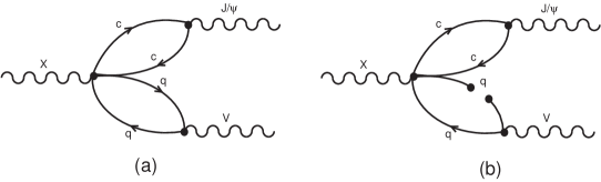
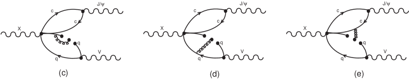
Figure 4: Diagrams which contribute to the OPE side of the sum rule.

In the OPE side we consider condensates up to dimension five , as shown in Fig. 4. Taking the limit $p^{2}={p^{\prime}}^{2}=-P^{2}$ and doing a single Borel transform to $P^{2}\rightarrow M^{2}$, we get in the structure $\epsilon^{\alpha\nu\sigma\gamma}p^{\prime}_{\sigma}q_{\gamma}p^{\prime}_{\mu}$ (the same considered in ref.decayx ) ($Q^{2}=-q^{2}$):

$$C(Q^{2})\left(e^{-m_{\psi}^{2}/M^{2}}-e^{-m_{X}^{2}/M^{2}}\right)+B~{}e^{-s_{0}/M^{2}}=$$

$$(Q^{2}+m_{\omega}^{2})\Pi^{(OPE)}(M^{2},Q^{2}),$$ (66)

where

$$\Pi^{(OPE)}(M^{2},Q^{2})={\langle\bar{q}q\rangle\over 6\sqrt{2}\pi^{2}Q^{2}}\bigg{[}\bigg{(}{m_{0}^{2}\over 3Q^{2}}+$$ (67)

$$- 1\bigg{)}\int_{4m_{c}^{2}}^{u_{0}}du~{}e^{-u/M^{2}}~{}\sqrt{1-4m_{c}^{2}/u}\left({1\over 2}+{m_{c}^{2}\over u}\right)+$$

$$- {m_{0}^{2}\over 16}\int_{0}^{1}d\alpha{1+3\alpha\over\alpha}~{}e^{-m_{c}^{2}\over\alpha(1-\alpha)M^{2}}\bigg{]}.$$

In Eq. (66)

$$C(Q^{2})={6\over\sin(\theta)}m_{\omega}f_{\omega}{f_{\psi}\lambda^{q}\over m_{\psi}(m_{X}^{2}-m_{\psi}^{2})}g_{X\psi\omega}(Q^{2}),$$ (68)

and $B$ gives the contribution of the pole-continuum transitions decayx ; dsdpi ; io2 . $s_{0}$ and $u_{0}$ are the continuum thresholds for $X$ and $J/\psi$ respectively. Notice that in Eq.(67) we have introduced the form factor $g_{X\psi\omega}(Q^{2})$. This is because the meson $\omega$ is off-shell in the vertex $XJ/\psi\omega$.

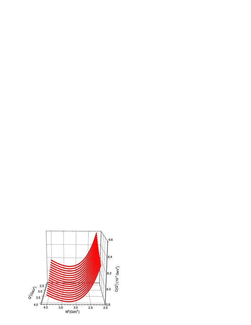
Figure 5: Values of $C(Q^{2})$ obtained by varying both $Q^{2}$ and $M^{2}$ in Eq. (66).

If we parametrize $C(Q^{2})$ as a monopole:

$$C(Q^{2})={c_{1}\over Q^{2}+c_{2}},$$ (69)

we can fit the left hand side of Eq. (66) as a function of $Q^{2}$ and $M^{2}$ to the QCDSR results in the right hand side, obtaining $c_{1}$, $c_{2}$ and $B$. In Fig. 5 we show the points obtained if we isolate $C(Q^{2})$ in Eq. (66) and vary both $Q^{2}$ and $M^{2}$. The function $C(Q^{2})$ (and consequently $g_{X\psi\omega}(Q^{2})$) should not depend on $M^{2}$, so we limit our fit region to $3.0\mbox{ GeV}^{2}\leq M^{2}\leq 3.5\mbox{ GeV}^{2}$ where $C(Q^{2})$ is clearly stable in $M^{2}$ for all values of $Q^{2}$.

We do the fitting for $s_{0}^{1/2}=4.4\mbox{ GeV}$ as the results do not depend much on this parameter, the results are shown bellow:

$$c_{1}=2.5\times 10^{-2}\mbox{ GeV}^{7},$$

$$c_{2}=38\mbox{ GeV}^{2},$$

$$B=2.9\times 10^{-4}\mbox{ GeV}^{5}.$$ (70)

In Fig. 6 we can see that the $Q^{2}$ dependence of $C(Q^{2})$ is well reproduced by the chosen parametrization in the interval $2.5\leq Q^{2}\leq 4.5~{}\mbox{ GeV}^{2}$, where the QCDSR is valid.

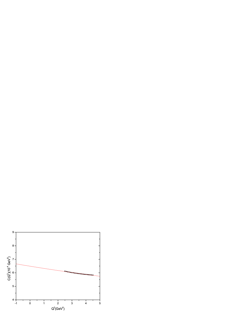
Figure 6: Momentum dependence of $C(Q^{2})$ for $s_{0}^{1/2}=4.4\mbox{ GeV}$. The solid line gives the parametrization of the QCDSR results (dots) through Eq. (69) and (70).

The form factor $g_{X\psi\omega}(Q^{2})$ can then be easily obtained by using Eqs. (68) and (69). Since the coupling constant is defined as the value of the form factor at the meson pole: $Q^{2}=-m_{\omega}^{2}$, to determine the coupling constant we have to extrapolate $g_{X\psi\omega}(Q^{2})$ to a $Q^{2}$ region where the sum rules are no longer valid (since the QCDSR results are valid in the deep Euclidian region). Using $m_{\psi}=3.1\mbox{ GeV}$, $m_{X}=3.87\mbox{ GeV}$, $f_{\psi}=0.405\mbox{ GeV}$, $\lambda^{u}=3.6\times 10^{3}\mbox{ GeV}^{5}$ from Eq. (36) and varying $\theta$ in the range $5^{\circ}\leq\theta\leq 13^{\circ}$, we get:

$$g_{X\psi\omega}=g_{X\psi\omega}(-m_{\omega}^{2})=5.4\pm 2.4$$ (71)

The decay width is given by:

$$\Gamma\left(X\rightarrow J/\psi\pi^{+}\pi^{-}\pi^{0}\right)=g_{X\psi\omega}^{2}{m_{\omega}\Gamma_{\omega}\over 8\pi^{2}m^{2}_{X}}B_{\omega\rightarrow\pi\pi\pi}I_{\omega},$$ (72)

which, together with Eq. (71) gives us:

$$\Gamma\left(X\rightarrow J/\psi\pi^{+}\pi^{-}\pi^{0}\right)=(9.3\pm 6.9)~{}\mbox{ MeV}.$$ (73)

The result in Eq. (73) is in complete agreement with the experimental upper limit. It is important to notice that the width grows with the mixing angle $\theta$, as can be seen from Eq. (68), while the mass grows with $\theta$. Therefore, there is only a small range for the values of this angle that can provide simultaneously good agreement with the experimental values of the mass and the decay width, and this range is $5^{\circ}\leq\theta\leq 13^{\circ}$. This means that the $X(3872)$ is basically a $c\bar{c}$ state with a small, but fundamental, admixture of molecular $DD^{*}$ states. By molecular states we mean an admixture between $D^{0}\bar{D}^{*0},~{}\bar{D}^{0}{D}^{*0}$ and $D^{+}D^{*-},~{}D^{-}D^{*+}$ states, as given by Eq. (59).

V Conclusions

We have presented a QCDSR analysis of the two-point and three-point functions of the $X(3872)$ meson, by considering a mixed charmonium-molecular current. We find that the sum rules results in Eqs. (35) and (73) are compatible with experimental data. These results were obtained by considering the mixing angle in Eq. (10) in the range $5^{\circ}\leq\theta\leq 13^{\circ}$.

We have also studied the mixing between the $D^{0}\bar{D}^{*0},~{}\bar{D}^{0}{D}^{*0}$ and $D^{+}D^{*-},~{}D^{-}D^{*+}$ states by imposing the ratio in Eq. (1). In accordance with the findings in ref. maiani we found that the mixing angle in Eq. (59) is $\alpha\sim 20^{0}$.

With the knowledge of these two mixing angles we conclude that the $X(3872)$ is basically a $c\bar{c}$ state ($\sim$97%) with a small, but fundamental, admixture of molecular $D^{0}\bar{D}^{*0},~{}\bar{D}^{0}{D}^{*0}$ ($\sim$88%) and $D^{+}D^{*-},~{}D^{-}D^{*+}$ ($\sim$12%) states.

This small molecular component could, in principle, be a consequence of neglecting the two-hadron reducible contribution in the phenomenological side. However, as argued in section III, we expect the 2HR contribution to be small and the results to hold even if we had taken it into consideration.

References

(1) S.-K. Choi et al. [Belle Collaboration],
Phys. Rev. Lett. 91, 262001 (2003).
(2) V. M. Abazov et al. [D0 Collaboration],
Phys. Rev. Lett. 93, 162002 (2004);
D. Acosta et al. [CDF Collaboration], Phys. Rev. Lett.
93, 072001 (2004);
B. Aubert et al. [BaBar Collaboration],
Phys. Rev. D 71, 071103 (2005).
(3)
K. Abe et al. [Belle Collaboration], hep-ex/0505037,
hep-ex/0505038.
(4) B. Aubert et al. [BaBar Collaboration],
Phys. Rev. D 74, 071101 (2006).
(5) D. Abulencia et al. [CDF Collaboration], Phys. Rev.
Lett. 96, 102002 (2006).
(6) D. Abulencia et al. [CDF Collaboration], Phys. Rev.
Lett. 98, 132002 (2007).
(7) T. Barnes and S. Godfrey, Phys. Rev. D 69, 054008 (2004).
(8) C. Cawfield et al. [CLEO Collaboration],
Phys. Rev. Lett. 98, 092002 (2007).
(9) F.E. Close and P.R. Page, Phys. Lett. B 578, 119
(2004).
(10) E.S. Swanson,
Phys. Rept. 429, 243 (2006).
(11) L. Maiani, F. Piccinini, A.D. Polosa, V. Riquer,
Phys. Rev. D 71, 014028 (2005).
(12) A.D. Polosa, arXiv:hep-ph/0609137.
(13) K. Abe et al. [Belle Collaboration], arXiv:0809.1224.
(14) B. Aubert et al. [BaBar Collaboration],
arXiv:0803.2838.
(15) R.D. Matheus, S. Narison, M. Nielsen and J.-M. Richard,
Phys. Rev. D 75, 014005 (2007).
(16) S.H. Lee, M. Nielsen and U. Wiedner, arXiv:0803.1168.
(17)
J. Sugiyama, T. Nakamura, N. Ishii, T. Nishikawa and M. Oka,
Phys. Rev. D 76, 114010 (2007)
[arXiv:0707.2533 [hep-ph]].
(18) M. Suzuki,
Phys. Rev. D 72, 114013 (2005).
(19) E.S. Swanson, Phys. Lett. B 588, 189 (2004); Phys. Lett.
B 598, 197 (2004).
(20) R. Li and K.-T. Chao, Phys. Rev. D 79, 114020
(2009).
(21) B.-Q. Li, C. Meng and K.-T. Chao, arXiv:0904.4068.
(22) Y.-R. Liu, X. Liu, W.-Z. Deng and S.-L. Zhu,
Eur. Phys. J. C 56, 63 (2008).
(23) Y. Dong, A. Faessler, T. Gutsche and V.E. Lyubovitskij,
Phys. Rev. D 77, 094013 (2008).
(24) Fl. Stancu, arXiv:0809.0408.
(25) B. Aubert et al. [BaBar Collaboration], Phys. Rev.
Lett. 102, 132001 (2009).
(26) M.A. Shifman, A.I. and Vainshtein and V.I. Zakharov,
Nucl. Phys. B 147, 385 (1979).
(27) L.J. Reinders, H. Rubinstein and S. Yazaki, Phys. Rept.
127, 1 (1985).
(28) For a review and references to original works, see
e.g., S.
Narison, QCD as a theory of hadrons,
Cambridge Monogr. Part. Phys. Nucl. Phys. Cosmol.17, 1 (2002)
[hep-h/0205006]; QCD
spectral sum rules , World Sci. Lect. Notes Phys.26, 1 (1989);
Acta Phys. Pol. B26, 687 (1995); Riv. Nuov. Cim. 10N2, 1
(1987); Phys. Rept. 84, 263 (1982).
(29) Y. Kondo, O. Morimatsu, T. Nishikawa, Phys. Lett. B611,
93 (2005).
(30) S.H. Lee, H. Kim, Y. Kwon, Phys. Lett. B609, 252 (2005).
(31) S. Narison, Phys. Lett. B466, 345 (1999);
S. Narison, Phys. Lett. B361, 121 (1995);
S. Narison, Phys. Lett. B387, 162 (1996); S. Narison, Phys. Lett.
B624, 223 (2005).
(32) K. Terasaki, arXiv:0904.3368.
(33) F.S. Navarra, M. Nielsen, Phys. Lett. B639, 272 (2006).
(34) D. Gamermann, E. Oset, arXiv:0905.0402.
(35) M. Nielsen, Phys. Lett. B634, 35 (2006).
(36) B. L. Ioffe and A.V. Smilga, Nucl. Phys. B232, 109
(1984).