Quantum scalar fields in the half-line.
A heat kernel/zeta function approach.

Abstract

In this paper we shall study vacuum fluctuations of a single scalar field with Dirichlet boundary conditions in a finite but very long line. The spectral heat kernel, the heat partition function and the spectral zeta function are calculated in terms of Riemann Theta functions, the error function, and hypergeometric ${}_{P}F_{Q}$ functions.

1 Introduction

In collaboration with J. Sesma, J. Abad devoted part of the last years of his fertile scientific career to studying the r$\hat{\rm o}$le of special functions in quantum field theory. In this brief memoir, elaborated to honor Julio’s memory, we explore the influence of using Dirichlet boundary conditions in quantum field theory. Specifically, we shall address the Higgs model in (1+1)-dimensions but we shall restrict the spatial line to become a finite interval. Then, Dirichlet boundary conditions at the endpoints of the interval will be imposed on the field. Eventually, we shall allow the length of the interval to tend to infinity to describe the situation in which the mesons meet an impenetrable wall. Our playground is thus the analysis of scalar quantum fields living in a half-line.

In this short work we shall concentrate on computing very basic quantities. Essentially, we shall deal with vacuum fluctuations in such a way that the spectral zeta function of the second-order differential operator governing small fluctuations around the vacuum will be used to regularize the divergent zero-point energy. The spectral information is also encoded in the associated $K$-heat partition function and $K$-heat kernel. These spectral functions permit a high-temperature asymptotic expansion, which, in turn, determines via the Mellin transform the meromorphic structure of the spectral zeta function in terms of the heat coefficients. The main sources of our approach are References [2], [3], and [4] as well as [7] and [8]. We hope that Julio would have been pleased with our results. In recent times he was one of those rare theorists trusted and praised by experimental and applied physicists.

2 The Higgs model in a line

In the $(1+1)$-dimensional toy Higgs model the action

$$S=\int\,dy^{2}\,\left\{{1\over 2}\frac{\partial\psi}{\partial y^{\mu}}\frac{\partial\psi}{\partial y_{\mu}}-{\lambda\over 4}(\psi^{2}(y_{0},y)-{m^{2}\over\lambda})^{2}\right\}$$

governs the dynamics of the scalar field $\psi(y_{0},y):{\mathbb{R}}^{1,1}\rightarrow{\mathbb{R}}$. We choose the metric $g_{\mu\nu}={\rm diag}(1,-1)$ in (1+1)-dimensional ${\mathbb{R}}^{1,1}$ Minkowskian space-time. In the natural system of units $\hbar=c=1$ the dimension of the field, the mass, and the coupling constant are respectively: $[\psi]=1$, $[\lambda]=[m^{2}]=L^{-2}$. In terms of non-dimensional space-time coordinates and fields

$$y^{\mu}\rightarrow y^{\mu}={\sqrt{2}\over m}\cdot x^{\mu}\hskip 42.67912pt;\hskip 42.67912pt\psi(y^{\mu})\rightarrow\psi(y^{\mu})={m\over\sqrt{\lambda}}\cdot\phi(x^{\mu})\qquad,$$

the action functional and the field equations of the $\lambda(\phi)^{4}_{2}$ model read:

$$S={m^{2}\over\lambda}\int\,dx^{2}\,\left\{{1\over 2}\frac{\partial\phi}{\partial x^{\mu}}\frac{\partial\phi}{\partial x_{\mu}}-{1\over 2}(\phi^{2}(x_{0},x)-1)^{2}\right\}$$

$$\frac{\partial^{2}\phi}{\partial x_{0}^{2}}(x_{0},x)-\frac{\partial^{2}\phi}{\partial x^{2}}(x_{0},x)=2\phi(x_{0},x)(1-\phi^{2}(x_{0},x))\qquad.$$

The shift of the scalar field from the homogeneous stable solution, $\phi(x^{\mu})=1+H(x^{\mu})$, leads to the action

$$S=\frac{m^{2}}{\lambda}\int\,d^{2}x\,\left\{\left[{1\over 2}\partial_{\mu}H\partial^{\mu}H-2H^{2}(x^{\mu})\right]-\left[2H^{3}(x^{\mu})+{1\over 2}H^{4}(x^{\mu})\right]\right\}\qquad,$$

which shows the spontaneous symmetry breakdown of the internal parity ${\mathbb{Z}}_{2}$ symmetry.

3 Zero point vacuum energy with Dirichlet boundary conditions

The linearized field equations

$$\frac{\partial^{2}\delta H}{\partial x_{0}^{2}}(x_{0},x)-\frac{\partial^{2}\delta H}{\partial x^{2}}(x_{0},x)+4\delta H(x_{0},x)=0$$ (1)

allow us to expand the Higgs field $\delta H(x_{0},x)$ as a linear superposition of solutions obtained by means of separation of variables:

$$\delta H(x_{0},x)=\frac{1}{m}\cdot\sqrt{\frac{\lambda}{l}}\sum_{k}{1\over\sqrt{2\omega(k)}}\left\{a(k)e^{-ik_{0}x_{0}}f(x;k)+a^{*}(k)e^{ik_{0}x_{0}}f^{*}(x;k)\right\}\qquad.$$ (2)

(2) is the general solution of (1) if the dispersion relation between the frequency and energy of the plane waves $k_{0}^{2}-k^{2}-4=0$ ($k_{0}=\omega(k)=\sqrt{k^{2}+4}$) holds. Of course, $f(x;k)$ are the eigenfunctions of the second-order fluctuation operator:

$$K_{0}=-{d^{2}\over dx^{2}}+4\qquad\qquad,\qquad K_{0}f(x;k)=\omega^{2}(k)f(x;k)\qquad.$$ (3)

In the normalization interval $I=[0,l\,]$, $l={mL\over\sqrt{2}}$, the spectrum of $K_{0}$ with Dirichlet boundary conditions (following the method developed in [9])

$$K_{0}f_{n}(x)=\omega_{n}^{2}f_{n}(x)\qquad,\qquad f_{n}(0)=f_{n}(l)=0\qquad$$

is:

$$k_{n}=\frac{\pi}{l}n\qquad,\qquad\omega_{n}^{2}={\pi^{2}\over l^{2}}n^{2}+4\qquad,\qquad f_{n}(x)=\sqrt{{2\over l}}\,\,{\rm sin}({\pi\over l}nx)\qquad,\qquad n\in{\mathbb{Z}}^{+}\qquad.$$

Therefore, the classical Hamiltonian is tantamount to an infinite number of oscillators given by the Fourier coefficients of these standing waves:

$$H^{(2)} = {m^{3}\over\sqrt{2}\lambda}\int\,dx\,\left\{{1\over 2}\frac{\partial\delta H}{\partial x_{0}}\cdot\frac{\partial\delta H}{\partial x_{0}}+{1\over 2}\frac{\partial\delta H}{\partial x}\cdot\frac{\partial\delta H}{\partial x}+\delta H(x_{0},x)\cdot\delta H(x_{0},x)\right\}$$

$$= {m\over 2\sqrt{2}}\sum_{n=1}^{\infty}\,\omega(k_{n})\left(\frac{}{}a^{*}(k_{n})a(k_{n})+a(k_{n})a^{*}(k_{n})\right)\qquad.$$

Canonical quantization $[{\hat{a}}(k_{n}),{\hat{a}}^{\dagger}(k_{m})]=\delta_{nm}$ promotes the Fourier coefficients to creation and annihilation operators and gives the free quantum Hamiltonian:

$$\hat{H}^{(2)}_{0}={m\over\sqrt{2}}\sum_{n=1}^{\infty}\,\omega(k_{n})\left(\hat{a}^{\dagger}(k_{n})\hat{a}(k_{n})+{1\over 2}\right)\qquad.$$

It is clear that the vacuum $\left(\hat{a}^{\dagger}(k_{n})|0>=0,\forall n\right)$ energy is not zero but:

$$\Delta E_{0}=<0|\hat{H}|0>={m\over 2\sqrt{2}}\sum_{n=1}^{\infty}\omega(k_{n})={m\over 2\sqrt{2}}{\rm Tr}_{D}K_{0}^{{1\over 2}}\hskip 28.45274pt,$$

a divergent quantity.

3.1 The heat function

Better expectations of convergence are offered by another spectral function, the $K_{0}$-heat function:

$${\rm Tr}_{D}e^{-\beta K_{0}}=\int_{0}^{l}\,dx\,K_{K_{0}}(x,x;\beta)=\sum_{n=1}^{\infty}\,e^{-\beta\left(\frac{\pi^{2}n^{2}}{l^{2}}+4\right)}$$ (4)

where $K_{K_{0}}(x,y;\beta)$ is the kernel of the $K_{0}$-heat equation

$$\left(\frac{\partial}{\partial\beta}+K_{0}\right)\Psi(\beta,x)=\left(\frac{\partial}{\partial\beta}-{\partial^{2}\over\partial x^{2}}+4\right)K_{K_{0}}(x,y;\beta)=0\qquad,\qquad K_{K_{0}}(x,y;0)=\delta(x-y)$$

and $\beta=\frac{m}{k_{B}T}$ is proportional to the inverse temperature. Moreover, via the Mellin transform the spectral zeta function is obtained:

$$\zeta_{K_{0}}(s)=\frac{1}{\Gamma(s)}\int_{0}^{\infty}\,d\beta\,\beta^{s-1}{\rm Tr}_{D}e^{-\beta K_{0}}=\sum_{n=1}^{\infty}\,\frac{1}{(\frac{\pi^{2}n^{2}}{l^{2}}+4)^{s}}\qquad.$$ (5)

We shall use this meromorphic function of the complex variable $s$ (and will return to this later) to regularize the divergent sum of vacuum fluctuations, $\Delta E_{0}$, by assigning to it the value of the series at a regular point in the $s$ complex plane.

3.1.1 Riemann Theta constants

The $K_{0}$-heat function is essentially given by a Riemann Theta constant:

$${\rm Tr}_{D}\,e^{-\beta\,K_{0}}=\sum_{n=1}^{\infty}\,e^{-\beta\,\omega_{n}^{2}}=\frac{e^{-4\beta}}{2}\left(\sum_{n=-\infty}^{\infty}\,{\rm exp}[-\beta\,\frac{\pi^{2}}{l^{2}}\,n^{2}]-1\right)=\frac{e^{-4\beta}}{2}\left(\Theta\left[\begin{array}[]{c}0\\ 0\end{array}\right](0|i\,\frac{\pi}{l^{2}}\,\beta)-1\right)\,\,.$$ (6)

Here, we denote the very well known Riemann or Jacobi Theta functions in the form:

$$\Theta\left[\begin{array}[]{c}a\\ b\end{array}\right](z|\tau)=\sum_{n=-\infty}^{\infty}\,{\rm exp}\left[2\pi i[(n+a)(z+b)+{1\over 2}(n+a)^{2}\tau]\right]\qquad,$$

$z\in{\mathbb{C}}\,\,\,,\,\,\,\tau\in{\mathbb{C}},{\rm Im}\tau>0\,\,\,,\,\,\,a,b=0,{1\over 2}$. Thus, we need the Riemann Theta function at the $z=0$ point (Theta constant), the modular parameter $\tau=i\frac{\pi}{l^{2}}\,\beta$ (determined by $\beta$ and $l$), and the “characteristics” $a=b=0$. Use of the Poisson formula

$$\Theta\left[\begin{array}[]{c}0\\ 0\end{array}\right](0,i\,\frac{\pi}{l^{2}}\,\beta)=\frac{l}{\sqrt{\pi\beta}}\,\,\Theta\left[\begin{array}[]{c}0\\ 0\end{array}\right](0,i\,\frac{l^{2}}{\pi\beta})$$

allows us to write the $K_{0}$-heat function in the new form:

$${\rm Tr}_{D}\,e^{-\beta\,K_{0}}=\frac{e^{-4\beta}}{2}\left(\frac{l}{\sqrt{\pi\beta}}\Theta\left[\begin{array}[]{c}0\\ 0\end{array}\right](0,i\,\frac{l^{2}}{\pi\beta})-1\right)\qquad.$$

From this, an asymptotic formula for the behavior of the $K_{0}$-heat function is obtained:

$$\Theta\left[\begin{array}[]{c}0\\ 0\end{array}\right](0,i\,\frac{l^{2}}{\pi\beta})\cong 1+{\cal O}(e^{-{c\over\beta}})\quad\Rightarrow\quad{\rm Tr}_{D}\,e^{-\beta\,K_{0}}\cong_{\beta\rightarrow 0}\frac{e^{-4\beta}}{2}\left(\frac{l}{\sqrt{\pi\beta}}-1\right)+{\cal O}(e^{-{c\over\beta}})\qquad.$$ (7)

3.1.2 Physicists’ derivation: the Error function

We now offer a derivation of the asymptotic formula by means of physicists’ techniques. The idea is to look at the problem when $l$ is very large: $l\,\rightarrow\,\infty$. The spectral density of the standing waves can be determined from the phase shifts $\delta^{D}(k)=-{\rm Si}(2kl)$ (${\rm Si}(x)$ is the sine integral function) due to the reflected waves:

$${\rm sin}\left(kl+\delta^{D}(k)\right)=0\qquad\equiv\qquad kl+\delta^{D}(k)=n\pi\quad,\quad n\in{\mathbb{Z}}^{+}$$

$$\rho_{K_{0}}^{D}(k)=\frac{dn}{dk}={l\over\pi}+{1\over\pi}.\frac{d\delta^{D}}{dk}(k)={l\over\pi}\left(1-\frac{{\rm sin}(2kl)}{kl}\right)\qquad.$$

Thus, we end with an integral, rather than a series, for the $K_{0}$-heat function in terms of the error function:

$${\rm Tr}_{D}\,e^{-\beta\,K_{0}}={l\over\pi}\int_{0}^{\infty}\,dk\,\left(1-\frac{{\rm sin}2kl}{kl}\right)\cdot e^{-\beta(k^{2}+4)}={e^{-4\beta}\over 2}\left({l\over\sqrt{\pi\beta}}-{\rm Erf}\left[{l\over\sqrt{\beta}}\right]\right)\qquad.$$ (8)

The high-temperature formula agrees perfectly with (7)

$${\rm Erf}[{l\over\sqrt{\beta}}]\cong_{\beta\rightarrow 0}\,1+{\cal O}(e^{-{c\over\beta}})\quad\Rightarrow\quad{\rm Tr}_{D}\,e^{-\beta\,K_{0}}\cong_{\beta\rightarrow 0}\frac{e^{-4\beta}}{2}\left(\frac{l}{\sqrt{\pi\beta}}-1\right)+{\cal O}(e^{-{c\over\beta}})$$

and, neglecting exponentially small contributions, we find the coefficients of the high-temperature expansion:

$${\rm Tr}_{D}\,e^{-\beta\,K_{0}} = e^{-4\beta}\cdot\left(\frac{l}{\sqrt{4\pi\beta}}-{1\over 2}{\rm Erf}[\frac{l}{\sqrt{\beta}}]\right)=e^{-4\beta}\cdot\sum_{n}\,c_{n}(K_{0})\,\beta^{n-{1\over 2}}\quad,\quad n\in\{0\}\cup{\mathbb{Z}}^{+}_{1/2}$$

$$\cong e^{-4\beta}\left({l\over\sqrt{4\pi}}-{1\over 2}+{\cal O}(e^{-{c\over\beta}})\right)\qquad,\qquad c_{0}(K_{0})=\frac{l}{\sqrt{4\pi}}\,\,,\quad c_{1/2}(K_{0})=-{1\over 2}\qquad,$$

$c_{n}(K_{0})=0\quad,\quad\forall\,n\geq 1\,\,$.

3.2 The spectral zeta function

3.2.1 Epstein zeta function

Mellin’s transform of the $K_{0}$-heat function (6) provides the spectral zeta function in terms of the Epstein zeta function $E(s,a|A)=\sum_{n=-\infty}^{\infty}\,\frac{1}{(An^{2}+a)^{s}}$:

$$\zeta_{K_{0}}^{D}(s) = {1\over\Gamma(s)}\int_{0}^{\infty}\,d\beta\,\beta^{s-1}\,{\rm Tr}_{D}\,e^{-\beta K_{0}}={1\over 2\Gamma(s)}\cdot\int_{0}^{\infty}\,d\beta\,\beta^{s-1}\,\left(\sum_{n=-\infty}^{\infty}\,e^{-\beta({\pi^{2}\over l^{2}}n^{2}+4)}-e^{-4\beta}\right)$$

$$= {1\over 2}\sum_{n=-\infty}^{\infty}\,\frac{1}{({\pi^{2}\over l^{2}}n^{2}+4)^{s}}-\frac{1}{2^{2s+1}}={1\over 2}\,E(s,4|{\pi^{2}\over l^{2}})-\frac{1}{2^{2s+1}}\qquad.$$

Mellin’s transform, however, of the Poisson inverted version

$$\zeta_{K_{0}}^{D}(s) = {1\over 2\Gamma(s)}\cdot\int_{0}^{\infty}\,d\beta\,\beta^{s-1}\,e^{-4\beta}\,\left({l\over\sqrt{\pi}}\beta^{-{1\over 2}}\sum_{n=-\infty}^{\infty}\,e^{-{l^{2}\over\beta}n^{2}}-1\right)$$ (9)

$$= \frac{1}{\sqrt{\pi}}\cdot\frac{\Gamma(s-1/2)}{4^{s}\Gamma(s)}+\frac{l}{2^{s-1/2}\Gamma(s)\sqrt{\pi}}\,\sum_{n\in{\mathbb{Z}}/\{0\}}\,(ln)^{s-1/2}\,K_{1/2-s}(4ln)-\frac{1}{2^{2s+1}}\quad.$$

gives the spectral zeta function as a series of modified Bessel functions of the second type. Moreover, formula (9) shows that there are poles of $\zeta_{K_{0}}^{D}(s)$ at the points

$$s=\frac{1}{2},-\frac{1}{2},-\frac{3}{2},-\frac{5}{2},-\frac{7}{2},\cdots,-\frac{2j+1}{2},\cdots,\qquad j\in{\mathbb{Z}}^{+}$$

because $K_{1/2-s}(4ln)$ are transcendental entire functions, i.e. holomorhic functions of $s$ in ${\mathbb{C}}/{\infty}$ with an essential singularity at $s=\infty$.

3.2.2 Physicists’ derivation: Hypergeometric ${}_{P}F_{Q}$ functions

Mellin’s transform of the (8) version of the $K_{0}$-heat function

$$\zeta_{K_{0}}^{D}(s) = {1\over\Gamma(s)}\cdot\int_{0}^{\infty}\,d\beta\,\beta^{s-1}\,{e^{-4\beta}\over 2}\left({l\over\sqrt{\pi\beta}}-{\rm Erf}\left[{l\over\sqrt{\beta}}\right]\right)$$ (10)

$$= {l\over\sqrt{4\pi}}\cdot\frac{\Gamma(s-1/2)}{\Gamma(s)}\left({1\over 2^{2s-1}}-{1\over 2^{2(s-1)}}\cdot{}_{1}F_{2}[1/2;3/2,3/2-s;4l^{2}]\right.$$

$$- \left.\frac{l^{2s-1}}{s}\cdot{}_{1}F_{2}[s;1/2+s,1+s;4l^{2}]\right)\quad,$$

supplies a third analytical expression of the spectral zeta function. Euler $\Gamma$ functions and hypergeometric ${}_{P}F_{Q}$ functions, with power expansion around $z=0$

$${}_{P}F_{Q}[a_{1},a_{2},\cdots,a_{p};b_{1},b_{2},\cdots,b_{q};z]=\sum_{k=0}^{\infty}\frac{(a_{1})_{k}(a_{2})_{k}\cdots(a_{p})_{k}}{(b_{1})_{k}(b_{2})_{k}\cdots(b_{q})_{k}}\cdot\frac{z^{k}}{k!}\qquad,$$

where $(a)_{k}=a(a+1)(a+2)\cdots(a+k-1)$ is the Pochhammer symbol, enter the third formula of $\zeta_{K_{0}}^{D}(s)$. It is clear that the physical point $s=-{1\over 2}$ is a pole of at least $\Gamma(s-{1\over 2})$. Other poles come from the other poles of $\Gamma(s-{1\over 2})$, $s-{1\over 2}=0,-2,-3,-4,-5,\cdots$, and the poles of ${}_{1}F_{2}[1/2;3/2,3/2-s;4l^{2}]$ and ${}_{1}F_{2}[s;1/2+s,1+s;4l^{2}]$, which are meromorphic functions of $s$. From the residue representation of these functions

$${}_{1}F_{2}[\frac{1}{2};\frac{3}{2},\frac{3}{2}-s;4l^{2}] = \frac{\Gamma(\frac{3}{2})\Gamma(\frac{3}{2}-s)}{\Gamma(\frac{1}{2})}\cdot\sum_{j=0}^{\infty}\,{\rm res}_{u}\left(\frac{\Gamma(\frac{1}{2}-u)(-4l^{2})^{u}}{\Gamma(\frac{3}{2}-u)\Gamma(\frac{3}{2}-s-u)}\Gamma(u)\right)(-j)$$

$${}_{1}F_{2}[s;\frac{1}{2}+s,1+s;4l^{2}] = \frac{\Gamma(\frac{1}{2}+s)\Gamma(1+s)}{\Gamma(s)}\cdot\sum_{j=0}^{\infty}\,{\rm res}_{u}\left(\frac{\Gamma(s-u)(-4l^{2})^{u}}{\Gamma(\frac{1}{2}+s-u)\Gamma(1+s-u)}\Gamma(u)\right)(-j)$$

we find poles when $3/2-s=-k_{1},1/2+s=-k_{2},1+s=-k_{3},k_{1},k_{2},k_{3}\in{\mathbb{Z}}^{+}\bigcup\{0\}$. All together, there are poles of $\zeta^{D}_{K_{0}}(s)$ at:

$$s=\cdots-5/2,-2,-3/2,-1,-1/2,1/2,3/2,5/2,7/2,\cdots\qquad.$$

3.3 The heat equation kernel

Finally, in this sub-Section we analyze how the $K_{0}$-heat function, henceforth the spectral zeta function, are obtained from the $K_{0}$-heat kernel.

3.3.1 Jacobi Theta functions

The $K_{0}$-heat equation kernel satisfying the Dirichlet boundary conditions

$$\left(\frac{\partial}{\partial\beta}-{\partial^{2}\over\partial x^{2}}+4\right)K_{K_{0}}^{D}(x,y;\beta)=0\,\,\,,\,\,\,K_{K_{0}}^{D}(x,y;0)=\delta(x-y)\quad,\quad K_{K_{0}}^{D}(0,y;\beta)=K_{K_{0}}^{D}(l,y;\beta)=0\,.$$ (11)

is:

$$K_{K_{0}}^{D}(x,y;\beta) = {2\over l}e^{-4\beta}\sum_{n=1}^{\infty}\,{\rm sin}({\pi\over l}nx){\rm sin}({\pi\over l}ny)\cdot e^{-\beta{\pi^{2}\over l^{2}}n^{2}}={e^{-4\beta}\over l}\sum_{n=-\infty}^{\infty}\,{\rm sin}({\pi\over l}nx){\rm sin}({\pi\over l}ny)\cdot e^{-\beta{\pi^{2}\over l^{2}}n^{2}}$$ (16)

$$= {e^{-4\beta}\over 2l}\sum_{n=-\infty}^{\infty}\,\left({\rm cos}({\pi\over l}n(x-y))-{\rm cos}({\pi\over l}n(x+y))\right)\cdot e^{-\beta{\pi^{2}\over l^{2}}n^{2}}$$

$$= {e^{-4\beta}\over 2l}\cdot\left(\Theta\left[\begin{array}[]{c}0\\ 0\end{array}\right](\frac{x-y}{2l}|i\frac{\pi}{l^{2}}\beta)-\Theta\left[\begin{array}[]{c}0\\ 0\end{array}\right](\frac{x+y}{2l}|i\frac{\pi}{l^{2}}\beta)\right)\qquad.$$

Alternatively, a modular transformation allows us to express the heat kernel in the new form:

$$K_{K_{0}}^{D}(x,y;\beta) = e^{-4\beta}\cdot{1\over\sqrt{4\pi\beta}}\cdot\left(e^{-{(x-y)^{2}\over 4\beta}}\Theta\left[\begin{array}[]{c}0\\ 0\end{array}\right](-il\frac{x-y}{2\beta}|i\frac{l^{2}}{\pi\beta})\right.$$

$$- \left.e^{-{(x+y)^{2}\over 4\beta}}\Theta\left[\begin{array}[]{c}0\\ 0\end{array}\right](-il\frac{x+y}{2\beta}|i\frac{l^{2}}{\pi\beta})\right)\qquad,$$

because the Jacobi theta functions involved are modular forms of weight $1/2$.

3.3.2 Physicists’ derivation: the Laplace transform

Another route to solve (11) is to look for solutions of the form

$$K_{K_{0}}^{D}(x,y;\beta)=K_{K_{0}}(x,y;\beta)+e^{-4\beta}D(x,y;\beta)$$ (19)

where

$$K_{K_{0}}(x,y;\beta)=\frac{e^{-4\beta}}{\sqrt{4\pi\beta}}\cdot{\rm exp}[-\frac{(x-y)^{2}}{4\beta}]$$

is the $K_{0}$-heat equation kernel with periodic boundary conditions. (19) complies with Dirichlet boundary conditions if:

$$D(x,y;0)=0\quad,\quad D(0,y;\beta)=-\frac{1}{\sqrt{4\pi\beta}}\cdot e^{-\frac{y^{2}}{4\beta}}\quad,\quad D(l,y;\beta)=-\frac{1}{\sqrt{4\pi\beta}}\cdot e^{-\frac{(l-y)^{2}}{4\beta}}\,\,.$$ (20)

The Dirichlet boundary conditions (20) force the Laplace transform of $D(x,y;\beta)$, $\bar{D}(x,y;s)=\int\,d\beta\,e^{-s\beta}D(x,y;\beta)$, to satisfy:

$$\bar{D}(0,y;s)=-\frac{e^{-\sqrt{s}y}}{2\sqrt{s}}\qquad,\qquad\bar{D}(l,y;s)=-\frac{e^{-\sqrt{s}(l-y)}}{2\sqrt{s}}\qquad.$$ (21)

Moreover, the ansatz (19) solves (11) if $\bar{D}(x,y;s)$ solves the Laplace equation:

$$\left(\frac{d^{2}}{dx^{2}}-s\right)\bar{D}(x,y;s)=0\qquad.$$ (22)

The general solution of (22) is

$$\bar{D}(x,y;s)=A(y)e^{-\sqrt{s}x}+B(y)e^{\sqrt{s}x}$$

which complies with (21) if:

$$\bar{D}(x,y;s)={1\over 2\sqrt{s}} \cdot \left[\frac{{\rm exp}[-\sqrt{s}(l+x-y)]-{\rm exp}[-\sqrt{s}(x+y-l)]}{e^{l\sqrt{s}}-e^{-l\sqrt{s}}}\right.$$ (23)

$$+ \left.\frac{{\rm exp}[-\sqrt{s}(l-x+y)]-{\rm exp}[-\sqrt{s}(l-x-y)]}{e^{l\sqrt{s}}-e^{-l\sqrt{s}}}\right]\qquad.$$

The last step is to take the inverse Laplace transform of $\bar{D}(x,y;s)$ as given in (23). To do this, it is convenient to write the common denominator as a power series expansion:

$$\frac{1}{e^{l\sqrt{s}}-e^{-l\sqrt{s}}}=\frac{e^{-l\sqrt{s}}}{1-e^{-2l\sqrt{s}}}=\sum_{n=0}^{\infty}\,(-1)^{n}e^{-(2n+1)l\sqrt{s}}\qquad,$$

or,

$$\bar{D}(x,y;s)=\frac{1}{2\sqrt{s}} \cdot \sum_{n=0}^{\infty}\,(-1)^{n}\,\left[{\rm exp}[-\sqrt{s}(2l(n+1)+x-y)]-{\rm exp}[-\sqrt{s}(2nl+x+y)]\right.$$

$$+ \left.{\rm exp}[-\sqrt{s}(2l(n+1)-x+y)]-{\rm exp}[-\sqrt{s}(2l(n+1)-x-y)]\right]\qquad.$$

The inverse Laplace transform of this is easy and gives:

$$D(x,y;\beta)=\frac{1}{\sqrt{4\pi\beta}} \cdot \sum_{n=0}^{\infty}\,(-1)^{n}\,\left[{\rm exp}[-\frac{(2l(n+1)+x-y)^{2}}{4\beta}]-{\rm exp}[-\frac{(2ln+x+y)^{2}}{4\beta}]\right.$$

$$+ \left.{\rm exp}[-\frac{(2l(n+1)-x+y)^{2}}{4\beta}]-{\rm exp}[-\frac{(2l(n+1)-x-y)^{2}}{4\beta}]\right]\qquad.$$

From this formula we derive the Dirichlet $K_{0}$-heat kernel at coinciding points

$$K_{K_{0}}^{D}(x,x;\beta)={e^{-4\beta}\over\sqrt{4\pi\beta}}\cdot\left[1+\sum_{n=0}^{\infty}\,(-1)^{n}\left(2e^{-\frac{l^{2}(n+1)^{2}}{\beta}}-e^{-\frac{(ln+x)^{2}}{\beta}}-e^{-\frac{(l(n+1)-x)^{2}}{\beta}}\right)\right]$$

which in turn provide the $K_{0}$ heat function through integration on the interval:

$${\rm Tr}_{D}e^{-\beta K_{0}} = \int_{0}^{l}\,dx\,K_{K_{0}}^{D}(x,x;\beta)={le^{-4\beta}\over\sqrt{4\pi\beta}}\left(1+2\sum_{n=0}^{\infty}\,(-1)^{n}\,e^{-\frac{l^{2}(n+1)^{2}}{\beta}}\right)$$ (24)

$$- {e^{-4\beta}\over\sqrt{4\pi\beta}}\cdot\sum_{n=0}^{\infty}\,(-1)^{n}\,\int_{0}^{l}\,dx\,\left\{e^{-\frac{(ln+x)^{2}}{\beta}}+e^{-\frac{(l(n+1)-x)^{2}}{\beta}}\right\}$$

$$= {le^{-4\beta}\over\sqrt{4\pi\beta}}\left(2-\Theta\left[\begin{array}[]{c}0\\ 1/2\end{array}\right](0|i\frac{l^{2}}{\pi\beta})\right)$$

$$- {e^{-4\beta}\over 2}\sum_{n=0}^{\infty}\,(-1)^{n}\,\left({\rm Erf}\left[\frac{l(n+1)}{\sqrt{\beta}}\right]-{\rm Erf}\left[\frac{ln}{\sqrt{\beta}}\right]\right)\,.$$

Because

$$\sum_{n=0}^{\infty}\,(-1)^{n}\,\left({\rm Erf}\left[\frac{l(n+1)}{\sqrt{\beta}}\right]-{\rm Erf}\left[\frac{ln}{\sqrt{\beta}}\right]\right)\cong_{\beta\to 0}1+{\cal O}(e^{-\frac{c}{\beta}})$$

we again find

$${\rm Tr}_{D}\,e^{-\beta\,K_{0}}\cong_{\beta\rightarrow 0}\frac{e^{-4\beta}}{2}\left(\frac{l}{\sqrt{\pi\beta}}-1\right)+{\cal O}(e^{-{c\over\beta}})$$

in the high-temperature regime.

4 Summary and outlook

In sum, we have found three different expressions for the $K_{0}$-heat function:

$${\rm Tr}_{D}e^{-\beta K_{0}}=\frac{e^{-4\beta}}{2}f_{1}(\frac{\pi}{l^{2}}\beta)=\frac{e^{-4\beta}}{2}f_{2}(\frac{\pi}{l^{2}}\beta)=\frac{e^{-4\beta}}{2}f_{3}(\frac{\pi}{l^{2}}\beta)$$

where

$$f_{1}(|\tau|) = \Theta\left[\begin{array}[]{c}0\\ 0\end{array}\right](0|\tau)-1\qquad,\qquad|\tau|=\frac{\pi}{l^{2}}\beta$$

$$f_{2}(|\tau|) = \frac{1}{\sqrt{|\tau|}}-{\rm Erf}[\sqrt{\frac{\pi}{|\tau|}}]$$

$$f_{3}(|\tau|) = \frac{2}{\sqrt{|\tau|}}\left(1-{1\over 2}\Theta\left[\begin{array}[]{c}0\\ 1/2\end{array}\right](0|-\frac{1}{\tau})\right)-\sum_{n=0}^{\infty}(-1)^{n}\left({\rm Erf}\left[(n+1)\sqrt{\frac{\pi}{|\tau|}}\right]-{\rm Erf}\left[n\sqrt{\frac{\pi}{|\tau|}}\right]\right)\quad.$$

    

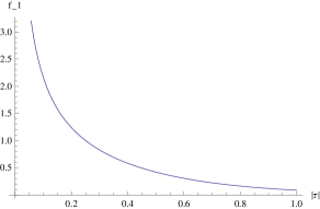
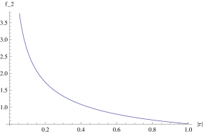
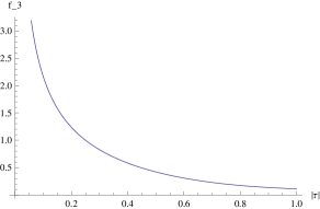
Figure 1: Plot of: a) $f_{1}(|\tau|)$, b)$f_{2}(|\tau|)$, and c) $f_{3}(|\tau|)$.

Figure 1 shows the Mathematica graphics of $f_{1}(|\tau|)$, $f_{2}(|\tau|)$ and $f_{3}(|\tau|)$. In Figure 2(a) the graphics of $f_{1}(|\tau|)$ and $f_{2}(|\tau|)$ are shown together. Simili modo, the graphics of $f_{1}(|\tau|$ and $f_{3}(|\tau|)$ are plotted together in Figure 2(b). It is clear that all three graphics agree perfectly when $\beta\to 0$ (high-temperature) and/or $l\to\infty$ (infinite length of the interval). $f_{1}(|\tau|)$ and $f_{2}(|\tau|)$, however, start to differ at $|\tau|=0.7$, whereas there are no differences in the graphics of $f_{1}(|\tau|)$ and $f_{3}(|\tau|)$. It is amazing how two different derivations involving highly sophisticated special functions lead to identical curves ! From a physical point of view we are tempted to speculate that $f_{3}(|\tau|)$ would give the exact result $f_{1}(|\tau|)$ because the infinite rebounds of the standing waves in the walls at $x=0$ and $x=l$ are accounted for. Instead, $f_{2}(x)$ counts a single rebound in the $x=0$ wall, which is a legitimate approximation for $l\to\infty$.

    

    

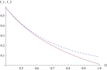
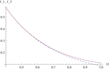
Figure 2: Plot of: (left) $f_{1}(|\tau|)$ (continuous line) and $f_{2}(|\tau|)$ (dashed line), and (right) $f_{1}(|\tau|)$ (continuous line) and $f_{3}(|\tau|)$ (dashed line).

We plan to follow this work by extending these computations to the kink sector of the model. The idea is to compute the one-loop kink mass shift in the framework developed in Reference [6] using Dirichlet boundary conditions instead of the periodic boundary conditions that are more conventional in quantum field theory . It will also be of great interest to perform the same program using more general families of boundary conditions, combining the method developed in [5, 6] with the formalism developed in references [7, 10, 9].

References

- [1]
- [2] E. Elizalde, Ten physical applications of spectral zeta functions, Springer Verlag, Berlin, 1995 .
- [3] K. Kirsten, Spectral functions in mathematics and physics, Chapman and Hall/CRC, New York, 2002 .
- [4] D. V. Vassilevich, Heat kernel expansion: user’s manual, Physics Report 388C (2003)279-360
- [5] A. Alonso Izquierdo, W. García Fuertes, M. A. González León, and J. Mateos Guilarte. Generalized zeta functions and one loop corrections to quantum kink masses. Nucl.Phys.B 635, 525 (2002). arXiv: hep-th/0201084.
- [6] A. Alonso Izquierdo, W. Garcia Fuertes, M. A. Gonzalez Leon, J. Mateos Guilarte, M. de la Torre Mayado, J. M. Muoz Castaeda, Lectures on the mass of topological solitons, arXiv: hep-th/0611180
- [7] M. Asorey, D. García-Álvarez, and J. M. Muoz-Castaeda. Casimir effect and global theory of boundary conditions, J.Phys.A.39,6127 (2006). arXiv: hep-th/0604089.
- [8] M. Asorey, D. García-Álvarez, and J. M. Muoz-Castaeda. Vacuum energy and renormalization on the edge. J.Phys.Conf.Ser.87:012004 (2007). arXiv: hep-th/07124353.
- [9] M. Asorey, and J. M. Muoz-Castaeda. Vacuum boundary effects. J.Phys.A.41,304004 (2008). arXiv: hep-th/08032553.
- [10] M. Asorey, G. Marmo, and J. M. Muoz-Castaeda. The world of boundaries without Casimir effect. To be published.