Abstract

The air-shower observatory Milagro has detected a large-scale anisotropy of unknown origin in the flux of TeV cosmic rays. We propose that this anisotropy is caused by galactic magnetic fields, in particular, that it results from the combined effects of the regular and the turbulent (fluctuating) magnetic fields in our vicinity. Instead of a diffusion equation, we integrate Boltzmann’s equation to show that the turbulence may define a preferred direction in the cosmic-ray propagation that is orthogonal to the local regular magnetic field. The approximate dipole anisotropy that we obtain explains well Milagro’s data.

1 Introduction

High-energy cosmic rays are of great interest in astrophysics, as they provide a complementary picture of the sky. When they are neutral particles (photons or neutrinos), they carry direct information from their source [1, 2, 3]. Gamma rays, in particular, have revealed during the past 30 years a large number of astrophysical sources (quasars, pulsars, blazars) in our Galaxy and beyond. In contrast, when they are charged particles (protons, electrons, and atomic nuclei) cosmic rays lose directionality due to interactions with the $\mu$G magnetic fields that they face along their trajectory [4]. In this case, however, they bring important information about the environment where they have propagated. For example, the simple observation that Boron is abundant in cosmic rays while rare in solar system nuclei is a very solid hint that cosmic rays have crossed around $10$ g/cm² of interstellar (baryonic) matter before they reach the Earth.

A very remarkable feature in the proton and nuclei fluxes is its isotropy. It is thought that cosmic rays of energy below $10^{6}$ GeV are mainly produced in supernova explosions, which are most frequent in the galactic arms. We observe, however, that they reach us equally from all directions. This can only be explained if their trajectories are close to the random walk typical of a particle in a gas, and galactic magnetic fields seem the key ingredient in order to justify this picture.

Galactic magnetic fields have been extensively reviewed in the literature [5, 6, 7, 8, 9]. It is known that there is an average magnetic field of order

$$B_{galactic}\approx 3\;\mu{\rm G}$$ (1)

at galactic scales. This component is the background to a second component of strength

$$B_{random}\approx 3\!-\!5\;\mu{\rm G}$$ (2)

that is regular within cells of 10–100 pc but changes randomly from cell to cell. These magnetic fields have frozen-in field lines and are very affected by the compressions and expansions of the interstellar medium produced by the passage of spiral arm waves. A 10 TeV cosmic proton would move inside a 5 $\mu$G field with a gyroradius of

$$r_{g}={p\over eB}\approx 2\times 10^{-3}\;{\rm pc}\;,$$ (3)

which is much smaller than the typical region of coherence. Therefore, this proton sees the superposition of both components as a regular magnetic field:

$$\vec{B}_{galactic}+\vec{B}_{random}=\vec{B}_{regular}\equiv\vec{B}\;.$$ (4)

Notice that the determination of the galactic field using WMAP data [10, 11, 12] gives $\vec{B}_{galactic}$. In contrast, estimates from Faraday rotations of pulsars would be sensitive to the same regular $\vec{B}$ that affects the cosmic proton. According to Han et al. [13, 8], the local $\vec{B}$ should be nearly contained in the galactic plane and clockwise as seen from the north galactic pole (i.e., following the direction of the disk rotation), although with a small vertical component or tilt angle.

At these small scales the 10 TeV proton is diffused by scattering on random fluctuations in the magnetic field

$$\delta B\ll B\;.$$ (5)

The interaction is of resonant character, so that the particle is predominantly scattered by those irregularities of the magnetic field of wave number $k\approx 1/r_{g}$. Estimates from the standard theory of plasma turbulence [14] indicate that $\delta B$ falls as a power law for larger wave numbers [13], so this component is smaller than the regular $B$.

In this paper we argue that the detailed observation of the TeV cosmic-ray flux obtained by Milagro [15, 16] may also provide valuable information about $\vec{B}$ and $\delta B$. In particular, the analysis of over $10^{11}$ air showers has produced a map of the sky showing a large-scale anisotropy (a north galactic deficit) of order $10^{-3}$. This map, which is consistent with previous observations [17, 18], remains basically unexplained. Abdo et al. [15, 16] have discussed several possible origins:

(i) The Compton-Getting (CG) effect [19], a dipole anisotropy that arises due to the motion of the Solar System around the galactic center and through the cosmic ray background. The anisotropy observed in Milagro’s map, however, cannot be fitted by the predicted CG dipole. In addition, the CG anisotropy should be energy independent, which does not agree with the data neither.

(ii) The heliosphere magnetic field could produce anisotropies [20, 21] that can also be ruled out. The Larmor radius $r_{g}$ sets the size of the coherence cells, and for 10 TeV protons it is around $2\times 10^{-3}$ pc, significantly larger than the $5\times 10^{-4}$ pc (100 AU) of the heliosphere. Moreover, as pointed out in [15, 16], the anisotropies persist at higher energies (i.e., for larger distance scales), supporting the hypothesis that if magnetic fields are involved they are extra-heliospheric.

Here we explore the effect of the local (regular and fluctuating) magnetic fields on the propagation of TeV cosmic rays reaching the Earth. Most analyses model cosmic-ray propagation with a diffusion equation [4, 22, 21], assuming certain spatial distribution of sources and a diffusion tensor often simplified to an isotropic scalar coefficient. This provides the flux over an extended region around the solar neighborhood. Here we intend a different approach. The diffusion equation derives from Boltzmann’s equation, which contains more information. The solution of Boltzmann’s equation in the vicinity of the Earth gives the statistical distribution function $f(\vec{r},\vec{p},t)$, a quantity related to the intensity or surface brightness used in astrophysics. $f$ provides the number of cosmic rays per unit solid angle, time and surface from any given direction, so it can be compared with Milagro’s data pixel by pixel.

2 Cosmic-ray distribution function

We will treat TeV cosmic rays as a fluid that microscopically interacts only with the magnetic fields, and our objective is to obtain the distribution function $f(\vec{r},\vec{p},t)$ using Boltzmann’s equation. We will take a basic cell of radius $r_{g}$ and will assume that the non-turbulent component of the fluid

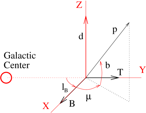
Figure 1: Angles $b$ and $\mu$, and orthogonal vectors $\vec{B}$, $\vec{T}$ and $\vec{d}$ for $l_{B}=90^{o}$.

is stationary and homogeneous. At these relatively small distance (and time) scales we can also neglect cosmic-ray sources, energy loss, or collisions with interstellar matter. In addition, we take the cosmic rays as protons (the dominant component in the flux) of $E=6$ TeV (the average energy in Milagro’s analysis). Finally, we will assume that the regular magnetic field $\vec{B}$ is on the galactic plane with a galactic longitude $l_{B}$, although we will show that Milagro’s data favors a component othogonal to this plane (as found in other observations [13]). In Fig. 1 we have depicted $\vec{B}$ with $l_{B}=90^{o}$.

The frequency of the $(b,\mu)$ direction in the momentum of cosmic rays reaching the Earth is then proportional to

$$f(\vec{u})=f(b,\mu)\;,$$ (6)

where $\vec{u}=\vec{p}/p$, $b$ is the galactic latitude, and $\mu$ is the longitude relative to the direction of the magnetic field $\vec{B}$. Notice that the galactic longitude of the direction defined by $\vec{u}$ is just $l=l_{B}+\mu$.

Boltzmann’s equation expresses in differential form how particles move in the six-dimensional phase space [23]. In our case this is just

$$\vec{F}\cdot\nabla_{\!u}\;f(\vec{u})=e\;(\vec{u}\times\vec{B})\cdot\nabla_{\!u}\;f(\vec{u})=0\;.$$ (7)

Now, we separate the regular and the turbulent components both in the distribution function and the magnetic field:

$$f \rightarrow f+\delta f\;,$$ (8)

$$\vec{B} \rightarrow \vec{B}+\delta\vec{B}\;.$$ (9)

The components $\delta\vec{B}$ and $\delta f$ vary randomly from one cell to another and have a vanishing average value,

$$\left[\delta\vec{B}\right]=\left[\delta f\right]=0\;.$$ (10)

However, there may be correlations between both fluctuating quantities. In particular, we will assume a non-zero value of

$$\left[e\;(\vec{u}\times\delta\vec{B})\cdot\nabla_{\!u}\;\delta f\right] = e\;\vec{u}\cdot\left[\delta\vec{B}\times\nabla_{\!u}\;\delta f\right]$$ (11)

$$= e\;\vec{u}\cdot\vec{T}$$ (12)

Boltzmann’s equation for the regular component is then

$$\left(\vec{u}\times\vec{B}\right)\cdot\nabla_{\!u}\;f+\vec{u}\cdot\vec{T}=0\;.$$ (13)

This equation can be also written

$$\vec{u}\cdot\left(\vec{B}\times\nabla_{\!u}\;f\right)+\vec{u}\cdot\vec{T}=0\;.$$ (14)

As $\vec{u}$ is any direction, this implies $\vec{B}\times\nabla_{\!u}\;f=\vec{T}$, i.e., the correlation $\vec{T}$ must be orthogonal to $\vec{B}$. Taking $\vec{T}$ in the galactic plane,

$$\vec{u}\cdot\vec{T}=T\;\cos b\;\sin\mu\;,$$ (15)

and expressing

$$\nabla_{\!u}\;f={\partial f\over\partial b}\;\vec{u}_{b}+{1\over\cos b}\;{\partial f\over\partial\mu}\;\vec{u}_{\mu}$$ (16)

with

$$\vec{u}_{b}=-\sin b\;\cos\mu\;\vec{u}_{\phi}-\sin b\;\sin\mu\;\vec{u}_{r}+\cos b\;\vec{u}_{z}\;;\;\;\;\vec{u}_{\mu}=-\sin\mu\;\vec{u}_{\phi}+\cos\mu\;\vec{u}_{r}\;,$$ (17)

Eq. (13) becomes

$$-\sin\mu\;{\partial f\over\partial b}+\tan b\;\cos\mu\;{\partial f\over\partial\mu}+{T\over B}\;\cos b\;\sin\mu=0\;.$$ (18)

This equation can be solved analytically:

$$f(b,\mu)=f_{0}\left(1+{T\over f_{0}B}\;\sin b\right)+\tilde{f}(\cos b\;\cos\mu)\;,$$ (19)

with $f_{0}$ a constant that normalizes $f$ to the number of particles per unit volume and the second term any arbitrary function of the variable $\cos b\;\cos\mu$. From the direction $\vec{u}$ we observe cosmic rays with $\vec{p}=-p\;\vec{u}$; it is straightforward to find the relation between the distribution function and the flux $F(b,\mu)$ of particles observed at Milagro per unit area, time, solid angle and energy:

$$F(b,\mu)={E^{2}\over c^{2}}\;f(-b,\mu+\pi)\;.$$ (20)

This implies

$$F(b,\mu)=F_{0}\left(1-t\;\sin b\right)+\tilde{F}(\cos b\;\cos\mu)\;,$$ (21)

where $t=T/(f_{0}B)$ and $F_{0}=(E/c)^{2}f_{0}$. Finally, we will expand $\tilde{F}$ to second order:

$$\tilde{F}(\cos b\;\cos\mu)\approx F_{1}\cos b\;\cos\mu+F_{2}\left(\cos b\;\cos\mu\right)^{2}\;.$$ (22)

The solution in terms of the galactic longitude is obtained just by expressing $\mu=l-l_{B}$.

Several comments are here in order.

(i) If $F_{1}=F_{2}=0$, then the solution is a dipole anisotropy, with the minimum/maximum in the north/south galactic poles. This dipole is then modulated by the constants $F_{1,2}$, that introduce an anisotropy proportional to $\cos b\cos\mu$ (i.e., the additional anisotropy coincides along the directions $\vec{u}$ with equal projection on $\vec{B}$).

(ii) The dipole anisotropy would vanish if there were no turbulence ($t=0$): $\vec{B}$ implies an isotropy broken by the turbulence in the orthogonal plane. In contrast, the equation does not say anything about the direction along $\vec{B}$. For different boundary conditions one can find solutions with a forward-backward asymmetry (implying diffusion along $\vec{B}$) or symmetric solutions. In particular, $F_{1}$ creates an asymmetry between the $(b=0,\mu=0)$ and $(b=0,\mu=180^{o})$ directions, whereas the $F_{2}$ contribution is symmetric.

(iii) The dominant magnetic field $\vec{B}$, the turbulence $\vec{T}$, and the dipole $\vec{d}$ are always orthogonal to each other. For $\vec{B}\approx B\vec{u}_{\phi}$ the symmetry of the galactic disc could favor a radial turbulence, $\vec{T}\approx T\vec{u}_{r}$, like the one that we have assumed above (see Fig. 1). However, one can change the latitude $b_{0}$ of the dipole while keeping $\vec{B}$ on the galactic plane just by taking the turbulence $\vec{T}$ out of the plane. In particular, the dipole will point towards the arbitrary direction $b_{0}$ (see Fig. 2) if

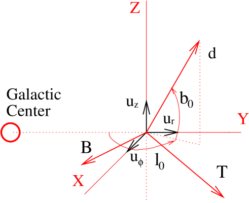
Figure 2: Trihedron defined by $\vec{B}$, $\vec{d}$ and $\vec{T}$, and coordinate system. $\vec{B}$ is in the galactic plane, whereas $\vec{d}$ and $\vec{T}$ have latitude $b_{0}$ and $90^{o}-b_{0}$, respectively.

$$\vec{u}\cdot\vec{T}=T\left(\sin b_{0}\;\cos b\;\sin\mu-\cos b_{0}\;\sin b\right)\;.$$ (23)

The dipole solution is in that case

$$F(b,\mu)= F_{0}\left[1-t\left(\sin b_{0}\;\sin b+\cos b_{0}\;\cos b\;\sin\mu\right)\right]$$ (24)

$$+F_{1}\cos b\;\cos\mu+F_{2}\left(\cos b\;\cos\mu\right)^{2}\;,$$ (25)

The galactic latitude $l_{0}$ of the dipole is then fixed by the orientation of $\vec{B}$ in the galactic plane,

$$l_{0}=l_{B}+90^{o}\;.$$ (26)

The direction of the dipole in the basis pictured in Fig. 2 is

$$\vec{u}_{d}=\cos b_{0}\;\sin l_{0}\;\vec{u}_{\phi}-\cos b_{0}\;\cos l_{0}\;\vec{u}_{r}+\sin b_{0}\;\vec{u}_{z}\;.$$ (27)

3 Milagro data

Milagro data [15] indicate a clear dipole anisotropy, with a deficit in the north galactic hemisphere that peaks at $\delta_{0}\approx 10^{o}$ and $AR_{0}\approx 190^{o}$ (i.e., $b_{0}\approx 72^{o}$ and $l_{0}\approx 293^{o}$). In Fig. 3 we plot our fit of the data (restricted to a region in the sky), which is

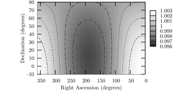
Figure 3: Fit of the Milagro anisotropy.

obtained for $t=0.003$ with $F_{1}/F_{0}=0$, $F_{2}/F_{0}=0.0003$ and a magnetic field $\vec{B}$ along $l_{B}=203^{o}$. Our simple fit, an approximate dipole along the direction of $\nabla_{u}f$ (from $b_{0}$, $l_{0}$ to $-b_{0}$, $l_{0}-\pi$) provides a good description of Milagro’s anisotropy.

The fit implies that cosmic rays move near the Earth with a mean velocity

$$\vec{v}_{0}/c=-{1\over N}\int{\rm d}\Omega\;F(\vec{u})\;\vec{u}=-0.00059\;\vec{u}_{\phi}-0.00028\;\vec{u}_{r}+0.00157\;\vec{u}_{z}$$ (28)

where $\;N=\int{\rm d}\Omega\;F(\vec{u})\;$ and the basis is pictured in Fig. 2. Eq. (28) expresses the diffusion velocity of the fluid (the transport flux $\vec{J}$ is proportional to $N\vec{v}_{0}$), and we find that it goes exactly in the direction of the dipole (the term $F_{1}$ would change its direction but we have set it to zero).

It is important to notice that the regular magnetic field $\vec{B}$ does not need to be on the galactic plane (our choice above), it can rotate around the dipole axis and still give the same dipole solution as far as the turbulence $\vec{T}$ is rotated as well. Doing that the only changes would appear in the boundary conditions ($F_{1}$ and $F_{2}$), but the pure dipole would provide the simplest solution in any case. The dipole seems to point towards

$$\vec{u}_{d}=-0.35\;\vec{u}_{\phi}-0.16\;\vec{u}_{r}+0.92\;\vec{u}_{z}\;.$$ (29)

Therefore, we can check if this dipole observed at Milagro and the local regular magnetic field $\vec{B}$ (also an observational output) are perpendicular. We will consider the values of $\vec{u}_{B}$ given by Han [13, 8]. It is found that $\vec{B}$ is basically azimuthal clockwise (a pitch angle of either $0^{o}$ or $180^{o}$ depending on the definition, which changes for different authors). However, the observations also indicate the presence of a non null tilt angle of $6^{o}$ (a vertical component of order 0.3 $\mu$G) taking the magnetic field out of the plane. We obtain an unitary vector

$$\vec{u}_{B}=0.99\;\vec{u}_{\phi}+0.00\;\vec{u}_{r}+0.10\;\vec{u}_{z}\;,$$ (30)

which implies a remarkable

$$\vec{u}_{d}\cdot\vec{u}_{B}=-0.18\;.$$ (31)

We think that the approximate orthogonality of these two observational vectors (we obtain an angle of $100^{o}$) provides support to the model presented here.

Notice that our framework could also accommodate other anisotropies in the flux, added to the dipole one, as far as they have the same value in all the points with equal projection ($\cos b\cos\mu$) on $\vec{B}$. To explain a pointlike anisotropy like the one named as region A in [16], the anisotropy itself should be along the direction of the dominant magnetic field $\vec{B}$ (orthogonal to $\vec{d}$). Region A, however, is at $(b_{A}\approx-30^{o},l_{A}\approx 215^{o})$, forming an angle of $58^{o}$ with the dipole.

4 Summary and discussion

Although charged cosmic rays do not reveal their source, the study of their flux from different directions is of interest in astrophysics because it brings valuable information about the interstellar medium. In particular, the per mille deficit observed by Milagro could be caused by the local (at distances of order $r_{g}$) magnetic fields.

Using Boltzmann’s equation we have shown that the interplay between the regular and the turbulent components in these magnetic fields always produces a dipole anisotropy in the cosmic-ray flux. We find that (i) the direction of this anisotropy is orthogonal to the regular $\vec{B}$ and (ii) its intensity is proportional to the fluctuations $\delta B/B$ at the wave number $k=1/r_{g}$. These two simple results have already non-trivial consequences. In particular, (i) implies that a north-south galactic anisotropy would only be consistent with a dominant $\vec{B}$ laying in the galactic plane, whereas (ii) explains that the anisotropy is larger for more energetic cosmic rays: their gyroradius $r_{g}$ is larger, the resonant wave number $k$ smaller, so the expected value of $\delta B/B$ will be larger.

We have argued that Milagro’s data can be interpreted as a dipole anisotropy pointing to a well defined direction in the north galactic hemisphere, namely, $(b_{0}\approx 67^{o},l_{0}\approx 284^{o})$. Our model provides a remarkable fit of the data, so we conclude that it explains satisfactorily the large-scale anisotropy found by Milagro. The model implies that the dominant magnetic field near our position must be in the plane orthogonal to the dipole ($\vec{B}$, the turbulence correlation $\vec{T}$ and $\vec{d}$ define a trihedron). This plane forms an angle $\theta=23^{o}$ with the galactic disc.

The data obtained by Milagro (energy, direction and nature of over $10^{11}$ primaries) shows that the $10^{-3}$ deficit in the cosmic-ray flux from the north galactic hemisphere already seen in previous experiments [17, 18] is actually very close to a dipole anisotropy. We think that the analysis of the flux after substracting this dipole anisotropy could reveal further correlations.

References

- [1] T. C. Weekes, “TeV Gamma-ray Astronomy: The Story So Far,” arXiv:0811.1197 [astro-ph];
- [2] H. J. Voelk and K. Bernloehr, “Imaging Very High Energy Gamma-Ray Telescopes,” arXiv:0812.4198 [astro-ph].
- [3] A. Achterberg et al. [IceCube Collaboration], Astropart. Phys. 26 (2006) 155.
- [4] A. W. Strong, I. V. Moskalenko and V. S. Ptuskin, Ann. Rev. Nucl. Part. Sci. 57 (2007) 285.
- [5] R. Beck, Astrophys. Space Sci. 289 (2004) 293.
- [6] R. Beck in Cosmic Magnetic Fields, Springer Verlag, Heidelberg, 2005. Edited by R. Wielebinski and R. Beck.
- [7] R. Wielebinski in Cosmic Magnetic Fields, Springer Verlag, Heidelberg, 2005. Edited by R. Wielebinski and R. Beck.
- [8] J. L. Han, “Magnetic structure of our Galaxy: A review of observations,” arXiv:0901.1165 [astro-ph].
- [9] E. Battaner in Lecture notes and essays in Astrophysics III, Tórculo, La Coruña, 2009. Edited by A. Ulla and M. Manteiga.
- [10] L. Page et al. [WMAP Collaboration], Astrophys. J. Suppl. 170 (2007) 335 [arXiv:astro-ph/0603450].
- [11] R. Jansson, G. R. Farrar, A. H. Waelkens and T. A. Ensslin, “Constraining models of the large scale Galactic magnetic field with WMAP5 polarization data and extragalactic Rotation Measure sources,” arXiv:0905.2228 [astro-ph.GA].
- [12] B. Ruiz-Granados, J.A. Rubiño-Martín and E. Battaner, “Determining the large-scale Galactic Magnetic Field pattern with 5-year WMAP polarization measurements at 22 GHz,” submitted to Astronomy and Astrophysics.
- [13] J. L. Han, R. N. Manchester, and G. J. Qiao, Month. Not. R.A.S. 306 (1999) 371.
- [14] F. Casse, M. Lemoine and G. Pelletier, Phys. Rev. D 65 (2002) 023002
- [15] A. A. Abdo et al., Astrophys. J. 698 (2009) 2121.
- [16] A. A. Abdo et al., Phys. Rev. Lett. 101 (2008) 221101.
- [17] M. Aglietta et al. [EAS-TOP Collaboration], Astrophys. J. 470 (1996) 501.
- [18] M. Amenomori [Tibet AS-gamma Collaboration], Science 314 (2006) 439.
- [19] A.H. Compton and I.A. Getting, Phys. Rev. 47 (1935) 817.
- [20] K. Nagashima, K. Fujimoto and R.M. Jacklyn, J. Geophys. Res. 103 (1998) 17429.
- [21] R. Schlickeiser, U. Dohle, R.C. Tautz and A. Shalchi, Astrophys. J. 661 (2007) 185.
- [22] V.S. Ptuskin, F.C. Jones, E.S. Seo and R. Sina, Adv. Space Res. 37 (2006) 1909.
- [23] E. Battaner, Astrophysical Fluid Dynamics, Cambridge University Press, New York, 1996.