Shock generated vorticity in the interstellar medium
and the origin of the stellar initial mass function

Abstract

Observations of the interstellar medium (ISM) and molecular clouds suggest these astrophysical flows are strongly turbulent. The main observational evidence for turbulence is the power-law energy spectrum for velocity fluctuations, $E(k)\propto k^{\alpha}$, with $\alpha\in[-1.5,-2.6]$. The Kolmogorov scaling exponent, $\alpha=-5/3$, is typical. At the same time, the observed probability distribution function (PDF) of gas densities in both the ISM as well as in molecular clouds is a log-normal distribution, which is similar to the initial mass function (IMF) that describes the distribution of stellar masses.

In this paper we examine the density and velocity structure of interstellar gas traversed by curved shock waves in the kinematic limit. We demonstrate mathematically that just a few passages of curved shock waves generically produces a log-normal density PDF. This explains the ubiquity of the log-normal PDF in many different numerical simulations. We also show that subsequent interaction with a spherical blast wave generates a power-law density distribution at high densities, qualitatively similar to the Salpeter power-law for the IMF. Finally, we show that a focused shock produces a downstream flow with energy spectrum exponent $\alpha=-2$. Subsequent shock passages reduce this slope, achieving $\alpha\approx-5/3$ after a few passages. We argue that subsequent dissipation of energy piled up at the small scales will act to maintain the spectrum very near to the Kolomogorov value despite the action of further shocks that would tend to reduce it. These results suggest that fully-developed turbulence may not be required to explain the observed energy spectrum and density PDF.

On the basis of these mathematical results, we argue that the self-similar spherical blast wave arising from expanding HII regions or stellar winds from massive stars may ultimately be responsible for creating the high mass, power-law, Salpeter-like tail on an otherwise a log-normal density PDF for gas in star forming regions. The IMF arises from the gravitational collapse of sufficiently overdense regions within this PDF. Thus, the composite nature of the IMF — a log-normal plus power-law distribution — is shown to be a natural consequence of shock interaction and feedback from the most massive stars that form in most regions of star formation in the galaxy.

1 Introduction

The distribution of stellar masses, known as the initial mass function (IMF), is of paramount importance to many fields of astrophysics. The form of the IMF plays a central role in subjects as diverse as galactic evolution and the formation and evolution of exoplanetary systems. Although its origin has been the focus of many analytical models for several decades, only recently have numerical simulations become available that can include many of the important physical processes involved (see the reviews by McKee & Ostriker, 2007; Bonnell et al., 2007). The form of the IMF is variously described as a log-normal distribution at low stellar masses with a power-law tail at masses exceeding a solar mass (e.g. Chabrier, 2003), or as a multiple power-law (e.g. Kroupa, 2002). The Salpeter power-law index of -1.35 for the high mass power-law tail appears to be universal. These properties of the IMF must ultimately reflect robust properties of the dense substructure within molecular clouds in the interstellar medium (ISM), in which stars are born.

It is not surprising therefore that one of the central problems in star formation is to characterize the mass distribution of the dense star-forming regions within clouds. Millimetre and submillimetre wave observations show that these clouds are highly inhomogeneous and are dominated by systems of filaments, punctuated by smaller denser regions in which clusters of stars form. Individual stars form in dense regions ($n\geq 10^{4}\mathrm{cm}^{-3}$ ), whose mass distribution is known as the core mass function (CMF). The gas velocities in these clouds are observed to be supersonic and chaotic. Numerical studies reveal that “turbulent” supersonic gas motions can reproduce many aspects of this structure. A number of observational surveys have shown that the CMF can be modelled by a log-normal distribution in many instances (e.g. Goodman et al., 2008). Other studies suggest that the high mass tail of this distribution is closer to a power-law, whose index is nearly identical to the Salpeter value (e.g. Motte et al., 1998; Johnstone et al., 2000). However, the debate continues as to the exact form of the mass distribution of these dense gaseous structures (e.g. Goodman et al., 2008).

This subject has made major advances largely due to the advent of numerical simulations. These show that the filamentary nature and the mass spectra of structure in clouds naturally result from the action of supersonic turbulence within them (e.g., the review of Mac Low & Klessen, 2004). The precise origin of the turbulence is still somewhat unclear. Molecular clouds are themselves embedded in a multi-component ISM and could be formed by several processes, including cloud collisions, spiral shock waves, and a combination of gravitational and magnetic instabilities. They are also shocked by the effects of feedback from star formation itself including expanding HII regions, supernovae, and powerful winds from massive stars. Simulations have started to make substantial progress in following most of these processes (e.g. Wada & Norman, 2001; Tasker & Bryan, 2006). The presence of supersonic turbulence within all molecular clouds has been interpreted as evidence that they are short lived structures that are dissipated in one or two shock crossing times: star formation occurs in the few transient turbulent structures that have sufficiently high density to collapse (e.g. Elmegreen, 2002; Hartmann et al., 2001). Indeed, observational studies of molecular clouds in the nearby LMC galaxy indicate that the time scale to form star clusters is rapid (of order a Myr) and that molecular clouds are rapidly dissipated in a few Myr as a consequence of their formation (Fukui et al., 1999). Turbulence within such clouds may result from processes on larger scales ($>100\mathrm{pc}$) that tap into energy released by galactic shear, gravitational instability or large-scale expanding HII regions.

In spite of the wide range of conditions in the interstellar medium and the details of the modelled process, time-dependent numerical simulations show that the density structure can be well modelled by a log-normal PDF over several orders of magnitude: from the diffuse atomic gas to molecular clouds (eg. Wada & Norman, 2007; Tasker & Bryan, 2008). At later times in their simulations of the ISM undergoing feedback from the effects of massive star formation Tasker & Bryan (2008) found that a power-law fit might also be possible. Numerical simulations of density fluctuations in purely isothermal supersonic turbulence have a log-normal PDF, and this is often taken as evidence for turbulence in the ISM. However, Padoan & Nordlund (2002) used the central limit theorem to show that a flow with a power-law energy spectrum will necessarily have a log-normal PDF of density. Thus, a log-normal PDF of density does not provide any more evidence for turbulence than a power-law energy spectrum.

How does the distribution of stellar masses arise from this density structure that characterizes the ISM? Stars are formed in fluctuations whose density exceeds a threshold for gravitational collapse. Recent theoretical work has emphasized that the shape of the IMF may be a combination of a power-law at large mass scales, that transitions to a log-normal form at lower masses. The peak of this distribution is a mass characteristic of gravitational collapse (e.g. Hennebelle & Chabrier, 2008; Padoan & Nordlund, 2002). The power-law tail and near Salpeter index for the mass function in molecular clouds has been modelled as arising from shocks generated in nearly Kolomogorov turbulence (e.g. Padoan & Nordlund, 2002), where the power-law index depends on the spectral index of the turbulent flow, and the half-width of the log-normal distribution depends on the turbulence Mach number. A recent analytic approach argues that the log-normal distribution for the IMF at low masses arises from that part of the gas density distribution that is supported by thermal pressure, whereas the Salpeter tail arises for higher mass cores that are supported by turbulent pressure (Hennebelle & Chabrier, 2008). An alternative explanation for a joint log-normal plus power-law distribution initial distribution is that an initial log-normal distribution can develop a power law tail if cores accrete over a distribution of time scales (Basu & Jones, 2004). Finally, Elmegreen (2002) noted that if one assumes that all gas above a density threshold in a log-normal distribution can form stars, then it is possible to recover the well-known Schmidt law that governs the global star formation rate in galaxies (see also Wada & Norman, 2007). .

In this paper, we examine the mathematical properties of shock-driven gas motions and propose a new approach to explain the nature of gas motions and density structure in the ISM and molecular clouds. We use analytical theory to examine both the density distribution expected in the gas due to the interaction of curved shocks, as well as the nature of the velocity fluctuations downstream of a shock. We show that the passage of just a few shock waves can very quickly establish log-normal density distributions. The passage of a spherical shock (i.e. blast wave) adds a power-law tail at large mass densities. We demonstrate that in general a log-normal distribution with a power-law at large densities is expected in media that are occasionally traversed by such large scale spherical shocks. These spherical shocks have been observed in the expanding HII regions that are a consequence of massive star formation. Thus, although gravity may be important for the large scale dynamics of molecular clouds (Goodman et al., 2008), the large scale shock waves of varying symmetry play an essential role in shaping the mass function of the cores.

The motions induced in the wake of curved shocks are vortical in nature. Power is distributed to vortical motions across a wide range of scales without a cascade process that is essential for Kolomogorov turbulence. Although tempting, we will argue that it is problematic to interpret the observations of Kolmogorov-like scaling in terms of hydrodynamic (or MHD) turbulence.

The paper is organized as follows. In §2 we contrast the properties of shock-driven and Kolmogorov turbulence. Then in §3 we review Kevlahan (1997)’s theory for vorticity generation by shocks propagating in nonuniform flows. Although it is commonly thought that straight shocks, weak shocks, and spherical shocks do not generate vorticity Kevlahan (1997) demonstrated that this is not true for shocks in inhomogeneous flows. In addition, we highlight the fact that curved shocks eventually focus. This focusing produces a pair of shock-shocks (Whitham, 1974) which generate vortex sheets downstream of the shock. This effect appears not to have been considered before in astrophysical flows. In §4 we show how multiple shock interactions could generate the observed log-normal and power-law distributions of mass density, and in §5 we show that the observed velocity energy spectra could be produced by the quasi-singular vorticity generated downstream of focused shocks and blast waves. Finally, we interpret the results in terms of an astrophysical model for the role of shock waves in generating density structure in the ISM and molecular clouds, and its connection to the IMF and close with our conclusions for shocks and star formation in the ISM §6.

2 Shock-driven flow and Kolmogorov turbulence

Observations of density and velocity fluctuations have suggested that many astrophysical flows are strongly turbulent. This phenomenon is widespread and includes a diverse set of systems — including H I emission in the interstellar medium (ISM), interstellar scintillations (ISS), 100$\mu$ IRAS emission in the interstellar medium (ISM) (Elmegreen & Scalo, 2004), velocity and density structure in molecular clouds, H I emission in the large Magellanic cloud (LMC) (Elmegreen et al., 2001), fluctuations in the solar wind (Horbury, 1999; Nicol et al., 2008), and hot H${{}_{2}}0$ emission in accretion disks (Carr et al., 2004). The evidence suggesting that these fluctuations are in fact turbulent is principally their turbulent-like velocity dispersions, or, equivalently, energy spectra and second-order structure functions, as well as their spatial density structure. Sometimes the scaling of higher-order structure functions is also taken as evidence of turbulence (e.g. Padoan et al., 2003). However, these results are not conclusive since there is still no rigorous theory for the scaling of high-order structure functions (only models, such as the one proposed by She & Leveque, 1994), and there is not enough data to obtain properly converged statistics for structure functions of order greater than about 6 or 7 without using the extended self-similarity (ESS) correction.

One of the central ideas in Kolmogorov’s classical theory of turbulence is that energy is injected at large scales and cascades without loss through intermediates scales, until it reaches the smallest scales where it is finally lost to molecular dissipation (see Elmegreen & Scalo, 2004, for a detailed review). Fully developed incompressible turbulence is characterized by a power-law energy spectrum $E(k)\propto k^{\alpha}$ where $\alpha=-5/3$ for incompressible homogeneous isotropic three-dimensional turbulence and $\alpha\in[-3,-4]$ for the enstrophy cascade in two-dimensional turbulence. Astrophysical fluctuations have observed power-law spectra with $\alpha\in[-1.5,-2.6]$ (Elmegreen & Scalo, 2004), suggestive of turbulence. Radio propagation observations of the diffuse ISM have found that density fluctuations obey the “Big power law in the sky”: Kolmogorov-like scaling of the energy spectrum extends over 11 orders of magnitude, from $10^{7}$cm to $10^{18}$ cm (Spangler, 1999)! However, Lazarian & Pogosyan (2000) comment that “the explanation of the spectrum as due to a Kolmogorov-type cascade faces substantial difficulties.” Indeed, they emphasize that “The existence of the Big Power Law (see Armstrong et al., 1995; Spangler, 1999) is one of the great astrophysical mysteries.”

Measurements of the velocity dispersion of gas within molecular clouds are made as a function of the size of the region in which the dispersion is measured. The data show that there is a power-law relation between the linewidth and size of a region such that $\Delta v\propto R^{\beta}$ (Ballesteros-Paredes et al., 2007). This scaling is a direct consequence of the energy spectrum since $\beta=-(\alpha+1)/2$. Larson (1981) first deduced that $\beta\simeq 0.38$, which is close to Kolmogorov turbulence $(\beta=1.3,\alpha=-5/3)$, and was the first to suggest that turbulence must play a very important role in the gas, and as a consequence, in the process of star formation that occurs in such clouds. Recent surveys for whole giant molecular clouds (GMCs) find $\beta\simeq 0.5-0.6$ (e.g. Heyer & Brunt, 2004), while studies of clouds with regions of low surface brightness find $\beta\simeq 0.4$ (Falgarone et al., 1992). Compressible gas motions which characterize the ISM are damped very quickly in shocks — typically in one crossing time of the driving scale.

Turbulence can also be characterized by the scaling of $\zeta_{p}$, the exponent of the $p-$th order structure function,

$$\langle|u(x+r)-u(x)|^{p}\rangle\propto r^{\zeta_{p}}.$$ (1)

Kolmogorov’s theory (Frisch, 1995) predicts that $\zeta_{p}$ is a linear function of $p$ (with $\zeta_{p}=p/3$). However, experiments show that $\zeta_{p}$ is in fact a concave function of $p$, increasing more slowly than linear with order $p$. Some attempts have been made to measure structure function exponents for astrophysical fluctuations (e.g. Nicol et al., 2008), although lack of data restricts the analysis to relatively low order ($p\leq 4$ or $6$) and quantitative comparison with turbulent flows is difficult since there is no accepted theory for how $\zeta_{p}$ should scale.

The equation of spectral energy balance for approximately incompressible homogeneous decaying turbulence is

$$\partial_{t}E(k)=-2\nu k^{2}E(k)+T(k),$$

where $k=|\bm{k}|$ is the magnitude of the wavenumber, the first term on the right hand side is viscous dissipation of energy (active only at small scales) and $T(k)$ measures the rate of energy transfer from all other wavenumbers $k^{\prime}$ to $k$ due to nonlinear interactions, i.e. it quantifies the energy cascade. Thus, in order to demonstrate conclusively the existence of an energy cascade one must estimate the energy transfer function,

$$T(k)=\int_{k=|\bm{k}|}\hat{\bm{u}}^{*}(\bm{k})\cdot\bm{P}(\bm{k})(\widehat{\bm{u}\times\bm{\omega}}(\bm{k}))\;\mathrm{d}S(k),$$

where $\hat{(\hskip 4.30554pt)}$ denotes the Fourier transform, $\bm{\omega}$ is the vorticity, $\bm{P}(\bm{k})$ is the divergence–free projection (for approximately incompressible flow) and the integral is over spherical shells in Fourier space. However, it is impossible to estimate $T(k)$ from the available the observational data since calculating $\bm{u}\times\bm{\omega}$ requires pointwise measurements of all components of the velocity and vorticity.

The interpretation of power-law scaling of the energy spectrum in terms of fully developed Kolmogorov turbulence in the ISM is problematic for several reasons.

1. Kolmogorov scaling is associated with incompressible neutral flow, whereas the ISM is believed to be strongly compressible and magnetic. Sridhar & Goldreich (1994) proposed a theory for anisotropic incompressible magnetohydrodynamic (MHD) turbulence which gives an energy spectrum $k_{\perp}^{-5/3}$ in directions perpendicular to the mean magnetic field. However, the theory is not rigorous and it does not apply to the solar wind. Other weak turbulence calculations find $k_{\perp}^{-2}$ or $k_{\perp}^{-3/2}$, and stationary constant flux solutions may have exponents anywhere in the range from $-1$ to $-3$ depending on the asymmetry of the forcing (Galtier et al., 2002).

2. The “Big power law in the sky” extends over a range of scales that include many different physical processes, including scales where the gas dynamics approximations of fluid turbulence are not valid. How can the same scaling be maintained across scales with very different physics?

3. It is not clear where the energy sustaining the ISM turbulence comes from. Candidates include massive stellar winds, supernovae, expanding HII regions, galactic rotation via spiral shocks, sonic reflection of shock waves hitting clouds, cosmic ray streaming, field star motions, Kelvin-Helmholtz and other fluid instabilities, thermal instabilities, gravitational instabilities, and galaxy interactions (Elmegreen & Scalo, 2004).

4. As pointed out by Lazarian & Pogosyan (2000), the damping rate of MHD turbulence is much faster than previously thought: about one eddy turnover time (as for neutral fluids). This implies very large energy injection scales and efficient and frequent forcing in order to sustain the turbulence (since the energy cascade takes about one eddy turnover time). It is useful to recall that hydrodynamic turbulence typically has constant or frequent forcing, e.g. vorticity generation via the no-slip boundary condition, or the mixing layer instability in jets. Vorticity generation occurs on a huge range of scales and does not require the lengthy process of an energy cascade.

In numerical simulations, on the other hand, turbulence is often generated via spiral shocks or super novae explosions (e.g. Joung & Mac Low, 2006; Piontek & Ostriker, 2005; Wada et al., 2002). This turbulence is necessarily limited to low Reynolds numbers, and the power-law scaling of the energy spectrum is present over a small range of scales (about a decade). Supersonic turbulence from these and other simulations of the ISM have a scaling close to the $-2$ associated with the shock discontinuity (Kritsuk et al., 2007; Vázquez-Semadeni et al., 1997).

Mathematically, the energy spectrum of a field is determined by its strongest singularity. If a function $f(x)$ has a discontinuity in the $p-1$ order derivative (where $p$ is an integer), then the energy spectrum of $f(x)$ has the form of a power-law

$$E(k)\sim k^{-2p}.$$

For example, a field containing shocks (discontinuities in the velocity field) has $E(k)\sim k^{-2}$. A singularity ‘worse’ than a discontinuity would be required to generate a slope shallower than $-5/3$, for example an accumulation of discontinuities around a given point, or a fractal (see Hunt et al., 1990). Note, however, that the converse is not true: smooth fields can have a power-law energy spectrum (e.g. adding together Gaussian functions of just the right size and amplitude could produce a $k^{-5/3}$ spectrum).

The fact that a power-law scaling is observed over such a wide range of scales suggests that a singularity may be responsible, such as the shocks that are ubiquitous in astrophysical flows. Kornreich & Scalo (2000) have proposed galactic shocks propagating through interstellar density fluctuations as a way of forcing (or “pumping”) supersonic turbulence. We go one step further: shock-generated vorticity alone may be enough to explain the observed energy spectra. Dynamical turbulence is not required.

As mentioned above, simulations of supersonic turbulence typically produce a $-2$ spectrum. This is not surprising since flows with turbulence Mach number $M_{t}>0.3$ will spontaneously generate shocklets (Kida & Orszag, 1990). Since the Kolmogorov $-5/3$ spectrum is likely not associated with a singularity, the $-2$ scaling dominates. However, as pointed out by Elmegreen & Scalo (2004), the observed spectra are often shallow than $-2$ and “the proposed shocks themselves have not been observed in real clouds.” In this paper we suggest a shock-based explanation of the observed spectra that addresses both these issues. First, we show that focused shocks generate vortex sheets, which means that the shock-driven flow may have a spectrum $E(k)\sim k^{-2}$ even when the shock is no longer present. Secondly, we show that multiple passages of curved shocks produces velocity fluctuations with a spectrum shallower than $-2$. Focused shocks are not the only shock structures that produce power-law scaling: we also find that multiple passages of strong spherical shocks produce similar results.

Dobbs & Bonnell (2007) have recently proposed a similar shock-based explanation of the velocity dispersion (i.e. energy spectrum) in molecular clouds. They use full smoothed particle hydrodynamics (SPH) simulations of the gas dynamics equations to show that shocks propagating through non-uniform fractal gas generate velocity dispersions close to the observed scaling. Our study is complementary: we use the full analytic expression for the vorticity produced by a curved shock in nonuniform flow to show that multiple shock passages could produce the observed velocity dispersion (and PDF of density fluctuations). We identify baroclinic vorticity generation as the key term. In addition, we find that fractal (or even non-uniform) initial conditions are not necessary.

3 Vorticity generation by curved and oblique shocks

In this section we review Kevlahan (1997)’s theory for the vorticity jump across a shock in non-uniform flow. We emphasize two effects that are usually neglected in discussions of vorticity generation by shocks: the creation of vortex sheets downstream of highly curved shock regions (e.g. shock–shocks), and the role played by non-uniformities in the flow ahead of the shock (which can lead to significant vorticity generation even by straight shocks).

The general expression for the vorticity jump in the binormal direction $\mathbf{b}$ across an unsteady three-dimensional shock moving into a non-uniform flow was derived by Hayes (1957),

$$\delta{\omega}\,\mathbf{b}=\mathbf{n}\times\left[-\frac{\partial(\rho C_{r})}{\partial S}\delta(\rho^{-1})(\rho C_{r})^{-1}(D_{S}\mathbf{U}_{S}+C_{r}D_{S}\mathbf{n})\delta(\rho)\right],$$ (2)

where $\bm{n}$ is the shock-normal direction, $\bm{s}$ is the tangential direction, and the binormal direction is given by $\bm{b}=\bm{s}\times\bm{n}$. Note that both $\bm{s}$ and $\bm{b}$ are tangential to the shock surface, and the normal component of the vorticity is continuous across a shock. $\partial/\partial S$ is the tangential part of the directional derivative, $C_{r}=C-A$ is the shock speed relative to the normal component of the flow ahead of the shock $A$, and $D_{S}$ is the tangential part of the total time derivative. A similar expression may be derived for the vorticity jump in the tangential direction $\mathbf{s}$. However, the expression usually taken for the vorticity jump is

$$\delta\omega\,\mathbf{b}=-\frac{\mu^{2}}{1+\mu}\mathbf{n}\times\left(\mathbf{U}_{S}\cdot\mathbf{K}+\frac{\partial C_{r}}{\partial S}\right)\mathbf{s},$$ (3)

where $\mu$ is the normalized density jump across the shock (the shock strength), $\mathbf{K}$ is the curvature of the shock and $\mathbf{U}_{S}$ is the velocity tangential to the shock in the reference frame of the shock. This expression was derived by Hayes from (2) by assuming that the flow ahead of the shock is uniform.

Kevlahan (1997) re-derived the vorticity jump equation, taking full account of terms due to the non-uniform upstream, finding that the vorticity jump in the binormal direction $\bm{b}$

$$\delta\bm{\omega}\cdot\bm{b}=\frac{\mu^{2}}{1+\mu}\frac{\partial C_{r}}{\partial S}-\frac{\mu}{C_{r}}\left(\left[\frac{D\bm{u}}{Dt}+\frac{C_{r}^{2}}{1+\mu}\frac{1}{\rho}\nabla\rho\right]\cdot\bm{s}\right)+\mu\bm{\omega}\cdot\bm{b},$$ (4)

together with a similar expression for the vorticity jump in the tangential direction $\bm{s}$. If the upstream flow is isentropic then $a_{0}^{2}/\rho\nabla\rho\approx-D\bm{u}/Dt$, and if, in addition, the upstream flow is quasi-steady and we normalize by the stagnation sound speed $a_{0}$ then (4) becomes

$$\delta\bm{\omega}\cdot\bm{b}=\frac{\mu^{2}}{1+\mu}\frac{\partial M_{s}}{\partial S}+\frac{1}{M_{s}}\left(\frac{\mu}{1+\mu}M_{s}^{2}-1\right)\left[\frac{\partial\frac{1}{2}M_{t}^{2}}{\partial S}+\bm{\omega}\times\bm{u}\cdot\bm{s}\right]+\mu\bm{\omega}\cdot\bm{b},$$ (5)

where $M_{t}$ is the turbulent Mach number of the upstream flow. We will use (5) in the remainder of the paper. Equation (5) may be simplified further for strong shocks by using the approximation $\mu\approx 2/(\gamma-1)$.

The density jump is given by

$$\delta\rho\equiv\mu\rho=\frac{M_{s}^{2}-1}{1+1/2(\gamma-1)M_{s}^{2}}\rho,$$ (6)

where $\mu$ is often referred to as the shock strength.

The first term on the right hand side of (5) represents vorticity generation due to the variation of the shock speed $M_{s}$ along the shock; by symmetry it is exactly zero for spherical and cylindrical shocks. Because shocks are nonlinear waves (unlike acoustic waves), $M_{s}$ is larger in regions of concave curvature and smaller in regions of convex curvature (with respect to the propagation direction of the shock). This difference in shock strength increases over time and eventually causes curved shocks to focus at regions of minimum curvature, developing a flat shock disk bounded by regions of very high curvature (often called kinks) (Kevlahan, 1996). In laboratory experiments shock focusing is obtained by reflecting a straight shock off a curved surface (see Sturtevant & Kulkarny, 1976, for a detailed discussion and pictures of shock focusing experiments). The discontinuous shock strength at the kinks is called a shock–shock. In the ISM shock focusing could arise due to reflection off density gradients (e.g. vertically stratified structure in disks), or due to small variations in shock curvature in blast waves.

As mentioned above, since the first term on the right hand side of (5) is approximately singular at the location of a kink, extremely strong jet-like vortex sheets develop in the flow downstream of the kinks (see figure 1). These vortex sheets themselves have an energy spectrum $E(k)\sim k^{-2}$, and generate turbulence exponentially fast via the Kelvin–Helmholtz instability. Note that this scenario produces a $-2$ spectrum in the downstream flow, even when the shock is no longer present (resolving the first objection mentioned in the introduction). In other words, the $-2$ spectrum is associated with the downstream flow, not with the shocks themselves (as has been assumed in the past).

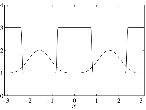
Figure 1: Focused shock model: — shock strength, - - - shock profile. Note the shock–shocks (discontinuities in shock strength) which generate vortex sheets in the downstream flow.

The second term on the right hand side of (5) is baroclinic generation of vorticity due to the misalignment of pressure and density gradients as the flow passes through the shock. This is the dominant term for vorticity production across straight or weakly curved shocks. It is also an important term in the case of multiple shock passages as it nonlinearly mixes the flow, redistributing energy amongst different length scales (similar the the quadratic nonlinearity of the Navier–Stokes equations). Note that vorticity may be generated across a straight shock even if the upstream flow is irrotational.

Finally, the third term on the right hand side of (5) is the additional angular momentum generated by compression of the flow in the direction normal to the front (i.e. conservation of angular momentum). This terms simply moves the entire energy spectrum up by the factor $\mu$ without changing its form.

The following sections use simple examples to show how multiple shock passages can generate density PDFs and energy spectra similar to what is seen in molecular clouds. We consider three generic shock types: weak eddy shocklets (which form spontaneously in supersonic turbulence), focused shocks, and strong spherical shocks (which model the blast waves generated by super novae explosions).

4 The distribution of mass density

In this section, we derive the density PDF of interstellar gas that results by the passage of various shock waves. We first demonstrate that a log-normal distribution is very rapidly established in a medium that is repeatedly lashed by multiple shock passages (§ 4.1). However, in § 4.2 we show that a power-law behaviour for a density PDF is expected for the passage of a perfectly spherical blast wave. Interstellar gas can therefore be regarded as being characterized by a log-normal density PDF, which from time to time develops a power-law tail at high densities due to the passage of a spherical blast wave from a nearby supernova, or an ongoing stellar wind bubble. This situation typifies the gas dynamics in regions of star formation.

4.1 Rapid generation of the log-normal density distribution

We first present a very simple explanation for the origin of the log-normal distribution of density commonly observed in isothermal turbulent flows. It is well-known that flows with $M_{t}>0.3$ spontaneously generate small, relatively weak and highly curved shocks, called ‘eddy shocklets’ Kida & Orszag (1990). It is therefore reasonable to assume that a region of space will be hit several times by shocklets of varying strengths. If we assume that the density is approximately stationary between shock passages (i.e. that the density changes primarily due to shock compression), then from equation (6) the density after $n$ shock passages is

$$\rho^{(n)}(x)=\prod_{j=0}^{n}(1+\mu^{(j)}(x))$$ (7)

where we have normalized density in units of the initial uniform density $\rho_{0}$. Let us consider the shock strengths $\mu^{(j)}(x)$ to be identically distributed random variables. Then, since $(1+\mu^{(j)}(x))>0$ we can take the logarithm of both sides and apply the central limit theorem to the resulting sum. This shows that the logarithm of density is normally distributed, i.e. the density PDF follows a log-normal distribution,

$$P(\rho)=\frac{1}{\sqrt{2\pi}\sigma\rho}\exp\left(-\frac{(\log(\rho)-\overline{\log\rho})^{2}}{2\sigma^{2}}\right).$$ (8)

Note that application of the central limit theorem to derive (8) requires only that the random variables $\log(1+\mu^{(j)}(x))$ have finite mean and variance.

One might think that it would take hundreds of shock interactions to converge to this log-normal distribution. However, if the PDF of density jumps is symmetric, then the rate of convergence is quite fast, $O(n^{-3/2})$. In fact, if the PDF of density jumps is uniform (a reasonable assumption) then, as shown in figure 2, as few as three or four shock passages generates a very good approximation to the log-normal distribution.

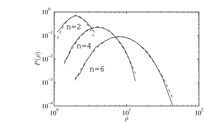
Figure 2: Convergence to a log-normal PDF of density after $n=2,4,6$ shock passages. - - -, log-normal distribution, — PDF of density.

In particular, if the PDF of density jumps $\mu$ is uniformly distributed in $(0,2/(\gamma-1)]$ (i.e. between its minimum and maximum possible values), then the logarithmic mean and variance of the log-normal distribution after $n$ shock passages are respectively

$$\overline{\log\rho} = \frac{n}{2}\ln\frac{\gamma+1}{\gamma-1},$$ (9)

$$\sigma^{2} = \frac{n}{12}\ln\frac{\gamma+1}{\gamma-1}.$$ (10)

There are two important aspects to these results. First, we see that both the mean and variance of the log-normal are largest for nearly isothermal gases (i.e. gases with $\gamma\approx 1$). Molecular gas can be well described as isothermal up to densities of $n\simeq 10^{9}$ cm^-3 due to efficient CO molecular as well as dust cooling. Second, the result shows that the logarithmic mean increases proportional to the number of shocks $n$ — and that the width of the distribution measured by the variance also grows proportional to $n$. These trends have been observed in the density PDFs of simulations of molecular clouds (e.g., the review of Mac Low & Klessen, 2004). The overall amplitude of the distribution decreases with growing $n$ simply because the integral of $P(\rho)$ must equal unity for any $n$. These trends are shown in figure 2. Note in particular how few shocks are required to establish a log-normal distribution to high accuracy. In a self-gravitating medium such as molecular gas, eventually gravity takes over and the dense cores begin to collapse.

The explanation for the log-normal distribution of density proposed here is even simpler and more general than that given previously by Nordlund & Padoan (1999). In fact, our results could explain Nordlund & Padoan (1999)’s observation that in a numerical simulation of isothermal supersonic turbulence “…the high-density wing of the Log-Normal is established very early – soon after the first shock interactions.” It is precisely these first few shock interactions that generate the log-normal distribution.

4.2 The power-law distribution at large densities

We have shown that interacting weak shocklets typical of supersonic turbulence quickly generate a log-normal PDF of mass density. However, observations show that the PDF of mass has a power-law tail at high masses with an exponent near the Salpeter index of -1.35. Although the mass and density PDFs are not identical, this observations suggests that the density PDF should also have a power tail at high densities. We show here that such a power-law tail may be explained by the interaction of the log-normal density fields of supersonic turbulence with a strong spherical shock (i.e. blast wave).

We adopt the solution for strong spherical shocks with sustained energy injection $E(t)\propto t^{p}$ derived by Dokuchaev (2002). This solution generalizes the Sedov–Taylor self-similar solution for a point blast explosion modelled by $p=0$ (i.e. an instant shock) to permanent energy injection modelled by $p=1$ (i.e. an injection shock). The first case corresponds to the instantaneous addition of energy to the ISM (as in a supernova explosion), while the second case corresponds to the continuous injection of energy (as in a massive stellar wind). The instant shock corresponds to the classical Sedov–Taylor solution for super novae explosions.

We assume  that the PDF of finding a particular value of gas density $\rho_{1}$ is proportional to the the space–time volume where the density exceeds $\rho_{1}$,

$$P(\rho>\rho_{1})\propto\int_{0}^{t(\rho_{1})}R^{3}(t)\,{\rm d}{t}$$ (11)

where $R(t)\propto t^{(2+p)/5}$ is the radius of the spherical shock at time $t$ and $t(\rho_{1})$ is the time at which the density behind the shock is equal to $\rho_{1}$. Using the relation $M_{s}(t)\propto R(t)/t$, equation (6) can be inverted to find $t(\rho_{1})\propto\rho^{5/(2(-3+p))}$.

Using the definition of the PDF, we find that the PDF of density due to the interaction of a homogeneous gas with a spherical blast wave has the form

$$P(\rho)=\frac{d}{d\rho}\int_{0}^{t(\rho)}R^{3}(t)\,{\rm d}{t}\propto\rho^{-(17+p)/(6-2p)}$$ (12)

(where we have re-labelled $\rho_{1}$ as $\rho$). Therefore, the density PDF is a power-law with exponent $-17/6\approx-2.8$ for an instant shock and $-9/2=-4.5$ for an injection shock. These slopes are significantly steeper than the Salpeter value for the mass PDF of $-1.35$. However, the actual relation between the density PDF and the mass PDF depends on the precise assumptions made about the scaling of clumps (i.e. mass equals density times a lengthscale cubed). Thus, one should not necessarily expect the same index for both the density and mass PDFs (although the power-law form should be robust).

Mathematically, the PDF of density resulting from the interaction of a spherical shock with a log-normally distributed density field is simply the convolution of the PDF (12) with the log-normal distribution of density (8). This produces a PDF which is log-normal for small densities, and has a power-law $\rho^{-(17+p)/(6-2p)}$ for high densities up to a maximum density proportional to $1/(\gamma-1)$. Figure 3 shows the resulting PDF, where the initial log-normal PDF is the result of four shocklet passages with maximum shock Mach number $M=1.5$ in a nearly isothermal gas with $\gamma=1.05$. It is important to note that because of the efficiency of CO and dust cooling, molecular gas remains essentially isothermal to density of $\simeq 10^{9}$ cm^-3 — hence our choice of an adiabatic index near to a value of unity.

Over time, the continuous production of shocklets will cause the PDF to revert to log-normal form, at the slower rate $O(n^{-1})$ (since the PDF is not symmetric). Thus, the presence of a power-law in the density PDF suggests that the flow has interacted recently with a blast wave (such as a super nova explosion).

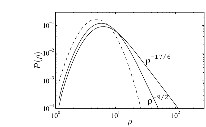
Figure 3: Generation of a power-law PDF at large densities in a nearly isothermal gas by a spherical blast wave interacting with a log-normally distributed density field. - - - is the initial log-normal PDF and the slopes -17/6 and -9/2 correspond to an instant shock and an injection shock respectively. Note that the upper limit of the power-law range is proportional to $1/(\gamma-1)$, and thus we expect the largest power-law ranges for nearly isothermal gases, i.e. those with $\gamma\approx 1$.

5 Energy spectrum

5.1 The multi-shock model

In addition to explaining the log-normal and power-law distributions of density, multiple shock interactions could also explain the observed power-law energy spectra (or velocity dispersion). It is important to emphasize that we consider the energy spectrum of the flow downstream of the shock. The velocity discontinuity associated with the shock itself gives $E(k)\propto k^{-2}$, which will determine the power-law exponent of the energy spectrum only if the downstream flow has an energy spectrum equal to or steeper than -2 (or unless there are no longer any shocks present). We will show that this is not the case in general for multiple shock passages. To the best of our knowledge, the special effects of focused shocks on the downstream flow have not been examined before in the astrophysical context.

The relevance of the case of multiple shock passages has been established by Kornreich & Scalo (2000), who found that the average time between shock passages in the ISM is “small enough that the shock pump is capable of sustaining supersonic motions against readjustment and dissipation.”

We use a semi-analytic approach to calculate the vorticity generation due to single and multiple passages of curved shocks. The vorticity jump is calculated using equation (5), and the velocity and the required gradients of upstream quantities are calculated using the fast Fourier transform (FFT) on a computational domain with periodic boundary conditions. The computational grid is $256^{3}$ in all cases. The initial flow is assumed to be irrotational.

We make the following assumptions:

1. Frozen vorticity: flow evolution is due to the shock alone. The flow is approximately steady between shock passages. This is similar to the rapid distortion approximation for strained turbulence, and it linearizes the problem. Kornreich & Scalo (2000) make a similar frozen vorticity assumption to neglect flow evolution during the shock passage. We deliberately ignore the internal dynamics of the flow: energy re-distribution amongst scales is due to the shock.

2. Strong shock: the shock does not change due to interaction with the flow.

3. Steady shock: the shock’s shape and strength distribution are fixed.

4. Random shock: The direction and phase of the shock are chosen randomly for each passage, and the results are averaged over many independent realizations. This is the same assumption we made in deriving the density PDFs.

This semi-analytic approach is extremely efficient numerically, and is similar to the kinematic simulation method for turbulence (Fung et al., 1992; Elliott & Majda, 1995) In kinematic simulation the energy spectrum is specified, but the complex phases are chosen randomly. Thus kinematic simulation is accurate for quantities that depend on second-order moments of the velocity field (e.g. particle dispersion and energy spectrum). However, as its name implies, kinematic simulation does not accurately represent the dynamics of a turbulent flow. In particular, the linearizing assumption that is at the heart of the model begins to break down once a significant amount of energy piles up at smaller scales. This will play an important role in defining the steepness of the energy distribution, as we shall see later in this section, and which will be discussed in the next.

The shock profile and shock strength profile for each case are described separately below.

5.2 Focused shocks and shock–shocks

We first consider flow driven by a focused shock. As mentioned in the introduction, a focused shock is characterized by a flattened shock disk bounded by two shock–shocks (or a shock–shock ring in the three-dimensional case). The shock strength is (approximately) discontinuous at the shock–shocks, which generate a vortex sheet (with spectrum $k^{-2}$) behind the shock. Vortex sheets are linearly unstable via the Kelvin–Helmholtz instability, and generate turbulence very efficiently and quickly.

We model the shock profile $\phi$ and shock speed $M_{s}$ by

$$\phi(x)=a\sin^{4}(k_{1}x)\hskip 150.00023pt$$ (13)

$$M_{s}(x)=M_{0}+1+\frac{4}{\pi}\sum^{n-1}_{j=1}\frac{(-1)^{j+1}}{(2j-1)}\cos\left((2j-1)2k_{1}x\right)\mathrm{sinc}^{2}\left(\frac{(2j-1)2k_{1}}{n}\right)$$ (14)

The expression for $M_{s}$ is simply the Fourier series for a square wave, where we have used the Lanczos $\sigma$-factor (the sinc term) to remove the Gibb’s oscillations. The number of terms $N$ in the series is taken equal to the number of Fourier modes used in the spectral method. We use a similar expression for a two-dimensional shock $z=\phi(x,y)$, with wavenumbers $k_{1}$ and $k_{2}$ in the $x$ and $y$ directions. Although this shock is simply a model (i.e. it is not the solution of the nonlinear wave equation governing shock motion), it captures its main qualitative features. The shock profile and shock strength are shown in figure 1.

We consider two initial conditions: a uniform flow (i.e. constant density and zero velocity), and an irrotational flow with a Gaussian energy spectrum $E(k)\propto\exp(-k^{2})$. The latter flow models the final decay regime of a turbulent flow, when viscous diffusion dominates.

Figure 4(a) shows the energy spectrum of the downstream three-dimensional flow after one, two and three passages of a focused shock with $k_{1}=k_{2}=1$, $M_{0}=6$ with zero velocity initial condition. Note that the initial $k^{-2}$ scaling of the energy spectrum (due to the velocity discontinuity associated with the vortex sheet downstream of the shock–shocks) becomes gradually shallower with each shock passage. This redistribution of energy to smaller scales is due to the quadratic baroclinic terms depending on the (inhomogeneous) upstream flow in the vorticity jump equation (5). Although the effect is entirely kinematic, these quadratic terms redistribute energy amongst scales in a way analogous to the quadratic nonlinearity in the Navier–Stokes equations.

After three shock passages the energy spectrum has a scaling similar to $k^{-5/3}$. More shock passages would produce an even shallower power-law. Figure 4(b) shows that the form of the energy spectrum is relatively insensitive to the choice of initial condition.

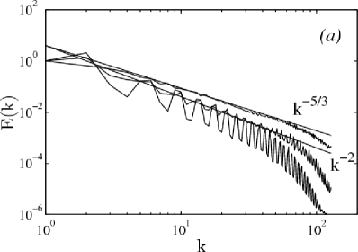
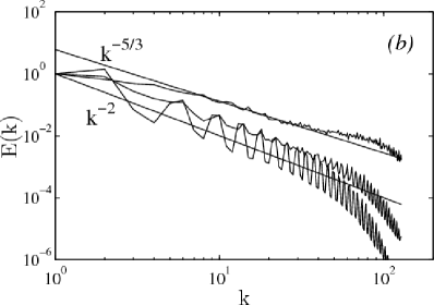
Figure 4: Energy spectra for multiple passages of focused shocks: slope decreases with each shock passage as energy is redistributed to smaller scales. Then spectra have been normalized so that $E(1)=1$. (a) Uniform initial flow. (b) Gaussian initial energy spectrum.

5.3 Spherical shocks

We now consider the case of perfectly spherical shocks described in §4.2. Due to symmetry, the shock strength $M_{s}$ is constant along the shock and therefore the first term in (5) is identically zero. This means that vorticity production is due entirely to the baroclinic and angular momentum conservation terms. Since the initial flow is irrotational, only the baroclinic term is active for the first shock, however subsequent shocks generate vorticity both baroclinically and via angular momentum conservation provided they are not coincident with the first shock.

For strong spherical shocks the vorticity jump (5) reduces to

$$\delta\bm{\omega}\cdot\bm{b}=\frac{2}{\gamma+1}M_{s}\left[\frac{\partial\frac{1}{2}M_{t}^{2}}{\partial S}+\bm{\omega}\times\bm{u}\cdot\bm{s}\right],$$ (15)

and thus, provided the upstream flow is non-uniform, the vorticity jump is proportional to $M_{s}(r)$.

If the upstream flow is smooth and irrotational, the energy spectrum of the downstream flow due to a single shock passage is simply the convolution of the Fourier transforms of the singular shock strength $M_{s}(r)$ given by Dokuchaev (2002)’s blast wave solution,

$$M_{s}(r)\propto r^{-(3-p)/(2+p)},$$ (16)

and the gradient of the turbulent kinetic energy (e.g. $k\exp(-k^{2})$). This gives $E(k)\sim k^{-3}$ for an instant shock and $E(k)\sim k^{-14/3}$ for an injection shock as $k\rightarrow\infty$. The energy spectrum for a generic self similar shock corresponding to (16) is

$$E(k)\sim k^{-(3+4p)/(1+p/2)}.$$ (17)

Recall that these are the energy spectra of the flow downstream of the shock.

The singularity at $r=0$ is removed by using the following regularization

$$M_{s}(r)=\frac{M_{s}(0)}{(1+(r/r_{min})^{2})^{\alpha/2}},$$ (18)

where the parameter $r_{min}$ is set slightly small than the grid size and $M_{s}(0)$ is set to ensure that $M_{s}=1$ at the edge of the computational domain. The upstream flow is assumed to be irrotational and to have a Gaussian energy spectrum $E(k)\propto\exp(-k^{2})$.

Figure 5 shows the energy spectrum of the downstream flow after one, two and three passages of a spherical instant shock and a spherical injection shock. Note that although the injection shock generates a much steeper energy spectrum after one passage ($k^{-14/3}$ compared to $k^{-3}$ for the instant shock), after three passages both spherical shock flows have a spectrum with a slope close to $-5/3$. As with the focused shocks, more shock passages would further decrease the slope as energy is redistributed to smaller scales by equation (15). This result is a consequence of our kinematic treatment. As we shall argue next, nonlinear processes will cut in to limit this evolution of the energy spectra.

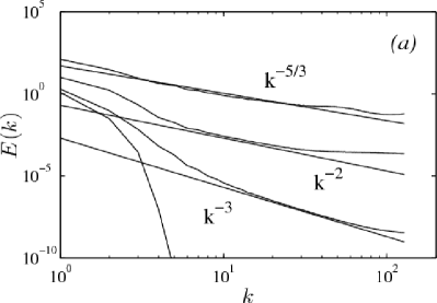
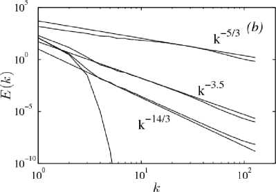
Figure 5: Energy spectra for multiple passages of spherical shocks: the slope decreases with each shock passage as energy is redistributed to smaller scales. The initial energy spectrum is Gaussian and all spectra have been normalized so that $E(1)=1$. (a) Instant shock ($p=0$). (b) Injection shock ($p=1$).

6 Astrophysical implications

While it is well known that curved shocks are an effective way of forcing a turbulent flow (Kornreich & Scalo, 2000), we have developed a simple kinematical model which demonstrates that shock interaction alone may can produce energy spectra of velocity fluctuations and mass density distributions consistent with the observations in the ISM. Fully developed turbulence is not necessary. Our result has several important implications for the density structure of gas in the ISM, and for the formation of stars within these structures.

6.1 Energy spectra

Simulations have confirmed that the structure observed in the interstellar medium and molecular clouds probably derives from shock-driven processes. Our results show that these processes do not drive turbulence in the classical sense of a systematic cascade in energy from large to small scales. The observed $E(k)\approx k^{-5/3}$ “big power-law in the sky” may actually be entirely shock-driven, and not a signature of fully-developed turbulence. This could explain why the power-law extends over such a huge range of length scales (spanning several different physical regimes, from the diffuse ISM to molecular gas), since the power-law of a shock-driven flow is due to a singularity, and so extends over all scales (until the viscous cut-off). Shock driven vortical motions are generic in the ISM, and we have shown that a log-normal ordering of gas structure develops rapidly over all scales of the gas. We demonstrated that this rapid appearance of a converged log-normal distribution is an expected property of shocked flows and the central limit theorem.

Our results also show that shocks should be much more efficient forcing the flow than has been appreciated previously. This is because the shock immediately distributes energy down to the smallest scales, according to a spectrum very close to the Kolmogorov -5/3 profile. Relying on a classical turbulent energy cascade is not feasible, since the time needed to transfer energy from the largest to the smallest scales (roughly one large-scale eddy turnover time) is far too slow.

How in this picture can a turbulence spectrum close to -5/3 be universal if repeated shocks can continue to make it shallower? As noted previously, continued steepening assumes a purely kinematic mechanism without the limitation of nonlinear or viscous effects. As we pointed out in the introduction, although radio propagation observations find a turbulence-like spectrum close to -5/3, the full set of astrophysical observations find spectra in the range $[-1.5,-2.6]$. So, our physical model needs to be able to produce a range of spectra, not just the single universal slope. Thus, we need to be able to suggest why -5/3 is the most likely spectrum, as well as accounting for other slopes.

There is in fact a natural limit to how shallow the slope can be. The slope could never become shallower than -1, since this would imply infinite energy (assuming an arbitrarily small minimum length scale). With each shock passage the slope of the energy spectrum becomes shallower as the shock redistributes energy to smaller scales (much as the nonlinear term of the Navier–Stokes equations does). In the kinematic limit this process would continue until the slope approaches -1. However, in reality once a sufficient amount of energy accumulates at the smallest scales energy dissipation by viscosity becomes significant. At this point, the linearizing assumptions of the kinematic model break down. Energy dissipation limits the continued transfer of energy to smaller scales, as well as driving an energy cascade to small scales (as in decaying turbulence). The energy cascade necessarily produces an energy spectrum that converges quickly to -5/3, since we now have the conditions required for the existence of a universal inertial range: a sink of energy at small scales separated from a wide and continuous range of active scales. The fact that the initial condition is already close to -5/3 means that we expect this adjustment to happen exponentially fast (as in the Kelvin–Helmholtz instability, where the initial spectrum is -2). Thus, the shock forcing effectively transfers energy to smaller and smaller scales until dissipation drives a turbulence cascade which fixes the slope of the energy spectrum at the universal value of -5/3.

The essential point is therefore that shock-generated vorticity will very quickly establish a power-law spectrum that is close to the Kolomogorov value. We argue that at this point, energy dissipation will tend to keep it there.

6.2 Feedback and the IMF

Another important result of our analysis concerns the appearance of a power-law tail for initially log-normal density PDFs that interact with spherical shock waves. The spherical symmetry means that a power-law will be imposed on the original log-normal distribution.

Consider the typical situation in a molecular cloud where a star cluster has started to form. We showed that the shock-driven motions that dominate an ISM with supersonic velocities rapidly produces a log-normal density PDF. It is well established that a typical star forms as a member of a star cluster (e.g. reviews by Pudritz, 2002; Lada & Lada, 2003). The collapse of the dense, gravitationally unstable regions results in the observed IMF. Before this process has terminated, however, a cluster is strongly impacted by the approximately spherical shocks associated with the most massive stars that have already formed nearby. Observations show that most embedded clusters are adjacent to HII regions that are excited by massive stars in nearby clusters (e.g. Elmegreen, 2002). Most clusters show evidence that their formation could, in fact, have been triggered by the powerful shock waves associated with the expansion of such nearby HII regions. We showed that the passage of these shocks alters the initial log-normal density PDF into one that has a power-law tail. This feedback from massive stars will therefore change the form of the IMF, most likely by producing a power-law tail.

Subsequent spherical shock passages will further modify the index of the power-law tail. We note, however that at most one or two passages would be expected since cluster formation is typically completed in a million years, which is roughly the crossing time for such an event. Thus, we conclude that feedback from massive stars is likely to leave a signature on the form of the density PDF in the gas which will carry over into the IMF (from those fluctuations that undergo gravitational collapse). Our analysis of how triggering may effect the form of the IMF given an initial gas density PDF will appear in a future paper.

An important caveat that we have not yet discussed is the possible role of magnetohydrodynamical (MHD) processes in shaping the density PDFs. Extensive sets of simulations have shown that magnetic fields with energy densities comparable to gravitational self-energy certainly can affect the form of the density PDF. However, the observations are best matched with fields strengths that are much less than this critical value. The simulations that best match the observations of dense magnetized cores involve “supercritical” field strengths, i.e. fields with significantly less energy density than gravitational and which are therefore subject to gravitational collapse (e.g. Padoan & Nordlund, 1999; Tilley & Pudritz, 2007; Crutcher et al., 2008) Thus, MHD effects in the bulk of molecular gas are probably far less pronounced than envisaged in earlier models of star formation.

Finally, and as technical aside, we suggest that it may be more useful numerically to generate a flow with the correct energy spectrum over a very wide range of lengthscales than to try to simulate the full nonlinear dynamics of a turbulent flow over a very small range of length scales (as is done currently). For example, Elliott & Majda (1995)’s method is able to efficiently generate a Gaussian random field with a $k^{-5/3}$ energy spectrum over 12 decades in two dimensions using only about 47 000 computational elements (compared to $10^{24}$ computational elements for a conventional non-adaptive approach!). In addition to being computationally efficient, this approach may actually be a better model of the hydrodynamics of the ISM.

7 Conclusions

Our results have important implications for the origin and evolution of density fluctuations, and particularly the CMF in molecular clouds. Our combined log-normal and power-law distribution arises because there are two natural kinds of symmetry to shocks — planar and spherical — that combine in a natural way. The fact that the power-law energy spectrum and log-normal distribution of mass density are also observed in the diffuse ISM strongly suggest that shock-generated vortical motions play a profound role on all scales in the ISM, and even in star formation within molecular clouds. Our specific conclusions are summarized below.

1. Supersonic turbulence with $M_{t}>0.3$ spontaneously generates relatively weak and short-lived ‘eddy shocklets’. A few passages of these shocklets is sufficient to generate a log-normal distribution of mass density. Thus, a log-normal distribution of density should be typical of supersonic turbulent flows, and is established very rapidly (the passage of just a couple of shocks will suffice). This is contrary to the usual assumption that enormous numbers of shock passages would be required due to the slow convergence to a normal distribution.

2. A spherical blast wave interacting with a log-normally distributed density field produces a power-law distribution of density at large densities, qualitatively similar to the observed Salpeter tail for the IMF. The power-law range increases like $1/(\gamma-1)$, and thus will be largest for nearly isothermal gases (i.e. those for which $\gamma\approx 1$). Over time the power-law gradually decays to a log-normal distribution due to the action of the continuously generated shocklets. Thus, the presence of a power-law in the density distribution implies that the flow has interacted fairly recently with a blast wave (e.g. supernova explosion).

3. A single strong shock passage can generate a relatively steep power-law energy spectrum over all length scales (e.g. $k^{-2}$ for a focused shock or $k^{-3}$ for a spherical blast wave) due to the singular structure of the shock strength. In the kinematic limit that we have investigated, subsequent shock passages increase the total energy and reduce the slope of the energy spectrum as the quadratic nonlinear term representing baroclinic generation of vorticity by the shock redistributes energy to smaller scales. Three shock passages suffice to produce an energy spectrum close to $k^{-5/3}$. Note that molecular clouds could not support more than a few large scale events, such as expanding HII regions, without being destroyed.

4. We argue that the onset of energy dissipation that is expected when energy piles up at the smaller scales acts to limit the energy spectrum generated by shocks to the Kolomogorov value.

5. The energy spectrum we find is that of the downstream flow, not that associated with the velocity jump of the shock itself (which has a $k^{-2}$ spectrum), i.e. we are not measuring the spectrum of the shock itself.

We close by noting that, to our knowledge, this is the first time vorticity generation and mass clumping by multiple hydrodynamic, curved shocks has been quantified analytically.

References

- Armstrong et al. (1995) Armstrong, J., Rickett, B., & Spang, S. 1995, ApJ, 443, 209
- Ballesteros-Paredes et al. (2007) Ballesteros-Paredes, J., Klessen, R. S., Mac Low, M.-M., & Vazquez-Semadeni, E. 2007, in Protostars and Planets V, ed. B. Reipurth, D. Jewitt, & K. Keil, 63–80
- Basu & Jones (2004) Basu, S. & Jones, C. E. 2004, MNRAS, 347, L47
- Bonnell et al. (2007) Bonnell, I. A., Larson, R. B., & Zinnecker, H. 2007, in Protostars and Planets V, ed. B. Reipurth, D. Jewitt, & K. Keil, 149–164
- Carr et al. (2004) Carr, J., Tokunaga, A., & Najita, J. 2004, ApJ, 603, 213
- Chabrier (2003) Chabrier, G. 2003, PASP, 115, 763
- Crutcher et al. (2008) Crutcher, R. M., Hakobian, N., & Troland, T. H. 2008, ArXiv e-prints
- Dobbs & Bonnell (2007) Dobbs, C. L. & Bonnell, I. A. 2007, Monthly Notices R. Astron. Soc., 374
- Dokuchaev (2002) Dokuchaev, V. 2002, Astron. & Astrophys., 395, 1023
- Elliott & Majda (1995) Elliott, F. & Majda, A. 1995, J. Comput. Phys., 117, 146
- Elmegreen et al. (2001) Elmegreen, B., Kim, S., & Staveley-Smith, L. 2001, ApJ, 548, 749
- Elmegreen & Scalo (2004) Elmegreen, B. & Scalo, J. 2004, Ann. Rev. Astron. Astrophys., 42, 211
- Elmegreen (2002) Elmegreen, B. G. 2002, ApJ, 577, 206
- Falgarone et al. (1992) Falgarone, E., Puget, J.-L., & Perault, M. 1992, A&A, 257, 715
- Frisch (1995) Frisch, U. 1995, Turbulence: the legacy of A.N. Kolmogorov (Cambridge University Press)
- Fukui et al. (1999) Fukui, Y., Mizuno, N., Yamaguchi, R., Mizuno, A., Onishi, T., Ogawa, H., Yonekura, Y., Kawamura, A., Tachihara, K., Xiao, K., Yamaguchi, N., Hara, A., Hayakawa, T., Kato, S., Abe, R., Saito, H., Mano, S., Matsunaga, K., Mine, Y., Moriguchi, Y., Aoyama, H., Asayama, S.-i., Yoshikawa, N., & Rubio, M. 1999, PASJ, 51, 745
- Fung et al. (1992) Fung, J. C. H., Hunt, J. C. R., Malik, N. A., & Perkins, R. J. 1992, J. Fluid Mech., 236, 281
- Galtier et al. (2002) Galtier, S., Nazarenko, S., Newell, A., & Pouquet, A. 2002, ApJ, 564, L49
- Goodman et al. (2008) Goodman, A. A., Pineda, J. E., & Schnee, S. L. 2008, ArXiv e-prints
- Hartmann et al. (2001) Hartmann, L., Ballesteros-Paredes, J., & Bergin, E. A. 2001, ApJ, 562, 852
- Hayes (1957) Hayes, W. 1957, J. Fluid Mech., 2, 595
- Hennebelle & Chabrier (2008) Hennebelle, P. & Chabrier, G. 2008, ApJ, 684, 395
- Heyer & Brunt (2004) Heyer, M. H. & Brunt, C. M. 2004, ApJ, 615, L45
- Horbury (1999) Horbury, T. 1999, in Plasma Turbulence and Energetic Particles in Astrophysics, Proceedings of the International Conference, Cracow (Poland), 5-10 September 1999, ed. M. Ostrowski & R. Schlickeiser, 115–133
- Hunt et al. (1990) Hunt, J., Vassilicos, J., Kevlahan, N.-R., & Farge, M. 1990, in Wavelets, fractals and Fourier transforms (Clarendon Press, Oxford), 1–38
- Johnstone et al. (2000) Johnstone, D., Wilson, C. D., Moriarty-Schieven, G., Joncas, G., Smith, G., Gregersen, E., & Fich, M. 2000, ApJ, 545, 327
- Joung & Mac Low (2006) Joung, M. K. R. & Mac Low, M.-M. 2006, ApJ, 653, 1266
- Kevlahan (1996) Kevlahan, N. K.-R. 1996, J. Fluid Mech., 327, 161
- Kevlahan (1997) —. 1997, J. Fluid Mech., 341, 371
- Kida & Orszag (1990) Kida, S. & Orszag, S. 1990, J. Sci. Comput., 5, 1
- Kornreich & Scalo (2000) Kornreich, P. & Scalo, J. 2000, ApJ, 531, 366
- Kritsuk et al. (2007) Kritsuk, A. G., Norman, M. L., Padoan, P., & Wagner, R. 2007, ApJ, 665, 416
- Kroupa (2002) Kroupa, P. 2002, Science, 295, 82
- Lada & Lada (2003) Lada, C. J. & Lada, E. A. 2003, ARA&A, 41, 57
- Larson (1981) Larson, R. B. 1981, MNRAS, 194, 809
- Lazarian & Pogosyan (2000) Lazarian, A. & Pogosyan, D. 2000, ApJ, 537, 720
- Mac Low & Klessen (2004) Mac Low, M.-M. & Klessen, R. S. 2004, Reviews of Modern Physics, 76, 125
- McKee & Ostriker (2007) McKee, C. F. & Ostriker, E. C. 2007, ARA&A, 45, 565
- Motte et al. (1998) Motte, F., Andre, P., & Neri, R. 1998, A&A, 336, 150
- Nicol et al. (2008) Nicol, R., Chapman, S., & Dendy, R. 2008, ApJ, 679, 862
- Nordlund & Padoan (1999) Nordlund, Å. K. & Padoan, P. 1999, in Interstellar Turbulence, ed. J. Franco & A. Carraminana, 218–+
- Padoan et al. (2003) Padoan, P., Boldyrev, S., Langer, W., & Nordlund, Å. 2003, ApJ, 583, 308
- Padoan & Nordlund (1999) Padoan, P. & Nordlund, Å. 1999, ApJ, 526, 279
- Padoan & Nordlund (2002) Padoan, P. & Nordlund, A. 2002, ApJ, 576, 870
- Piontek & Ostriker (2005) Piontek, R. & Ostriker, E. 2005, ApJ, 629, 849
- Pudritz (2002) Pudritz, R. 2002, Science, 295, 68
- She & Leveque (1994) She, Z.-S. & Leveque, E. 1994, Phys. Rev. Lett., 72, 336
- Spangler (1999) Spangler, S. 1999, in Plasma Turbulence and Energetic Particles in Astrophysics, Proceedings of the International Conference, Cracow (Poland), 5-10 September 1999, ed. M. Ostrowski & R. Schlickeiser, 1–4
- Sridhar & Goldreich (1994) Sridhar, S. & Goldreich, P. 1994, ApJ, 432, 612
- Sturtevant & Kulkarny (1976) Sturtevant, B. & Kulkarny, V. 1976, J. Fluid Mech., 73, 651
- Tasker & Bryan (2006) Tasker, E. J. & Bryan, G. L. 2006, ApJ, 641, 878
- Tasker & Bryan (2008) —. 2008, ApJ, 673, 810
- Tilley & Pudritz (2007) Tilley, D. A. & Pudritz, R. E. 2007, MNRAS, 382, 73
- Vázquez-Semadeni et al. (1997) Vázquez-Semadeni, E., Ballesteros-Paredes, J., & Rodríguez, L. 1997, ApJ, 474, 292
- Wada et al. (2002) Wada, K., Meurer, G., & Norman, C. 2002, ApJ, 577, 197
- Wada & Norman (2001) Wada, K. & Norman, C. A. 2001, ApJ, 547, 172
- Wada & Norman (2007) —. 2007, ApJ, 660, 276
- Whitham (1974) Whitham, G. 1974, Linear and nonlinear waves (John Wiley & Sons)