Distributed anonymous function computation in information fusion and multiagent systems

Abstract

We propose a model for deterministic distributed function computation by a network of identical and anonymous nodes, with bounded computation and storage capabilities that do not scale with the network size. Our goal is to characterize the class of functions that can be computed within this model. In our main result, we exhibit a class of non-computable functions, and prove that every function outside this class can at least be approximated. The problem of computing averages in a distributed manner plays a central role in our development.

1 Introduction

The goal of many multi-agent systems, distributed computation algorithms and decentralized data fusion methods is to have a set of nodes compute a common value based on initial values or observations at each node. Towards this purpose, the nodes, which we will sometimes refer to as agents, perform some internal computations and repeatedly communicate with each other. Let us consider some examples.

(a) Quantized consensus: Suppose that each agent begins with an integer value $x_{i}(0){\in\{0,\ldots,K\}}$. We would like the agents to end up, at some later time, with values $y_{i}$ that are almost equal, i.e., $|y_{i}-y_{j}|\leq 1$, for all $i,j$, while preserving the sum of the values, i.e., $\sum_{i=1}^{n}x_{i}(0)=\sum_{{i=1}}^{n}y_{i}$. This is the so-called quantized averaging problem which has received considerable attention recently; see [16, 9, 3, 20]. It may be viewed as the problem of computing the function $(1/n)\sum_{i=1}^{n}x_{i}$, rounded to the nearest integer.

(b) Distributed hypothesis testing: Consider $n$ sensors interested in deciding between two hypotheses, $H_{0}$ and $H_{1}$. Each sensor collects measurements and makes a preliminary decision $x_{i}\in\{0,1\}$ in favor of one of the hypotheses. The sensors would like to make a final decision by majority vote, in which case they need to compute the indicator function of the event $\sum_{i=1}^{n}x_{i}\geq n/2$, in a distributed way. Alternatively, in a weighted majority vote, they may be interested in computing the indicator function of the event $\sum_{i=1}^{n}x_{i}\geq 3n/4$.

(c) Solitude verification: This is the problem of verifying that at most one node in the network has a given state. This problem is of interest if we want to avoid simultaneous transmissions over a common channel [13], or if we want to maintain a single leader (as in motion coordination — see for example [15]) Given $K$ possible states, so that $x_{i}\in\{1,\ldots,{K}\}$, solitude verification is equivalent to the problem of computing the binary function which is equal to 1 if and only if $|\{i:x_{i}=1\}|=1$.

There are numerous methods that have been proposed for solving problems such as the above. (See for example the vast and growing literature on consensus and averaging methods.) Oftentimes, different algorithms involve different computational capabilities on the part of the agents, which makes it hard to talk about “the best” algorithm. At the same time, simple algorithms (such as setting up a spanning tree and aggregate information by progressive summations over the tree) are often “disqualified” because they require too much coordination or global information. One then realizes that a sound discussion of such issues requires the specification of a precise model of computation, followed by a systematic analysis of fundamental limitations under any given model. This is precisely the objective of this paper: to propose a particular model, and to characterize the class of computable functions under this model.

Our model provides an abstraction for the most common requirements for distributed algorithms in the sensor network literature. It is somewhat special because (i) it does not allow for randomization; (ii) it does not address the case of time-varying interconnection graphs; such extensions are left for future research. Qualitatively speaking, our model includes the following features.

Identical agents: Any two agents with the same number of neighbors must run the same algorithm.

Anonymity: An agent can distinguish its neighbors using its own, private, local identifiers. However, agents do not have global identifiers.

Absence of global information: Agents have no global information, and do not even have an upper bound on the total number of nodes. Accordingly, the algorithm that each agent is running is independent of the network size and topology.

Convergence: Agents hold an estimated output, and this estimate must converge to a desired value which is generally a function of all agents’ initial observations or values. In particular, for the case of discrete outputs, all agents must eventually settle on the desired value. On the other hand, the agents do not need to be aware of such termination, which is anyway impossible in the absence of any global information [6].

1.1 Goal and Contribution

We provide in this paper a general model of decentralized anonymous computation with the above described features, and characterize the type of functions of the initial values that can be computed. To keep our model simple, we only consider deterministic and synchronized agents exchanging messages on a fixed bi-directional network, with no time-delays or unreliable transmissions. Agents are modelled as finite automata, so that their individual capabilities remain bounded as the number of agents increases.

We prove that if a function is computable under our model, then its value only depends on the frequencies of the different possible initial values. For example, if the initial values $x_{i}$ only take values $0$ and $1$, a computable function necessarily only depends on $p_{0}:=|\{i:x_{i}=0\}|/n$ and $p_{1}:=|\{i:x_{i}=1\}|/n$. In particular, determining the number of nodes, or whether at least two nodes have an initial value of $1$ is impossible.

Conversely, we prove that if a function only depends on the frequencies of the different possible initial values (and is measurable), then the function can at least be approximated with any given precision, except possibly on a set of frequency vectors of arbitrarily small volume. Moreover, if the dependence on these frequencies can be expressed by a combination of linear inequalities with rational coefficients, then the function is computable exactly. In particular, the functions involved in the quantized consensus and distributed hypothesis testing examples are computable, whereas the function involved in solitude verification is not. Similarly, statistical measures such as the standard deviation and the kurtosis can be approximated with arbitrary precision.

Finally, we show that with infinite memory, the frequencies of the different values (i.e., $p_{0},p_{1}$ in the binary case) are computable.

1.2 Overview of previous work

There is a large literature on distributed function computation in related models of computation. A common model in the distributed computing literature involves the requirement that all processes terminate when the desired output is produced. A consequence of the termination requirement is that nodes typically need to know the network size $n$ (or an upper bound on $n$) to compute any non-constant functions. We refer the reader to [1, 6, 31, 17, 26] for some fundamental results in this setting, and to [10] for an excellent summary of known results.

Similarly, the biologically-inspired “population algorithm” model of distributed computation has some features in common with our model, namely finite-size agents and lack of a termination condition; see [2] for a very nice summary of known results. However, these models involve a somewhat different type of agent interactions from the ones we consider.

We note that the impossibility of computing $p_{1}$ without any memory was shown in [21]. Some experimental memoryless algorithms were proposed in the physics literature [12]. Randomized algorithms for computing particular functions were investigated in [16, 7]. We also point the reader to the literature on “quantized averaging,” which often tends to involve similar themes [9, 20, 3, 8].

Several papers quantified the performance of simple heuristics for computing specific functions, typically in randomized settings. We refer the reader to [14] and [29], which studied simple heuristics for computing the majority function. A deterministic algorithm for computing the majority function (and some more generalized functions) was proposed in [23].

Semi-centralized versions of the problem, in which the nodes ultimately transmit to a fusion center, have often be considered in the literature, e.g., for distributed statistical inference [25] or detection [19]. The papers [11], [18], and [22] consider the complexity of computing a function and communicating its value to a sink node. We refer the reader to the references therein for an overview of existing results in such semi-centralized settings.

Our results differ from previous works in several key respects: (i) Our model, which involves totally decentralized computation, deterministic algorithms, and constraints on memory and computation resources at the nodes, but does not require the nodes to know when the computation is over, does not seem to have been studied before. (ii) Our focus is on identifying computable and non-computable functions under our model, and we achieve a nearly tight separation.

2 Formal description of the model

The system consists of (i) a communication graph $G=(V,E)$, which is bidirectional (i.e., if $(i,j)\in E$, then $(j,i)\in E$); (ii) a port labeling whereby edges outgoing from node $i$ are labeled by port numbers in the set $\{1,2,\ldots,{\rm degree}(i)\}$; (iii) a family of finite automata $(A_{d})_{d=1,2,3,\ldots}$. (The automaton $A_{d}$ is meant to describe the behavior of a node with degree $d$.)

The state of the automaton $A_{d}$ is a tuple $(x,z,y,m_{1},\ldots,m_{d})$; we will call $x\in X{=\{0,1,\ldots,K\}}$ the initial value, $z\in{Z_{d}}$ the internal memory state, $y\in Y$ the output or estimated answer, and $m_{1},\ldots,m_{d}\in M$ the messages. The sets $X,Y,Z_{d},M$ are assumed finite, unless there is a statement to the contrary. Furthermore, we assume that the number of bits that can be stored at a node is proportional to the node’s degree; that is, $\log|Z_{d}|\leq Cd$, for some absolute constant $C$. (Clearly, at least this much memory would be needed to be able to store the messages received at the previous time step.) We will also assume that $\emptyset$ is an element of the above defined sets $Y$, $Z_{d}$, and $M$. The transition law $A_{d}$ maps $X\times{Z_{d}}\times Y\times M^{d}$ to $X\times{Z_{d}}\times Y\times M^{d}$: $\left[x,z,y;(m_{1},\dots,m_{d})\right]$ is mapped to $\left[x,z^{\prime},y^{\prime};(m^{\prime}_{1},\dots,m^{\prime}_{d})\right].$ In words, the automaton creates a new memory state, output, and (outgoing) messages at each iteration, but does not change the initial value.

We construct a dynamical system out of the above elements as follows. Let $d(i)$ be the degree of node $i$. Node $i$ begins with an initial value $x_{i}\in X$; it implements the automaton $A_{d(i)}$, initialized with $x=x_{i}$, and with $z=y=m_{1}=\ldots=m_{d}=\emptyset$. We use $S_{i}(t)=[{x_{i}},y_{i}(t),z_{i}(t),m_{i,1}(t),\ldots,m_{i,d(i)}(t)]$ to denote the state of the automaton implemented by agent $i$ at round $t$. Let $j_{1},\ldots,j_{d(i)}$ be an enumeration of the neighbors of $i$, and let $p_{k}$ be the port number of the link $(j_{k},i)$. The evolution of the system is then described by

$$\left[x_{i},z_{i}(t+1),y_{i}(t+1);m_{i,1}(t+1),\ldots,m_{i,d(i)}({t+1})\right]=A_{d(i)}\left[x,z_{i}(t),y_{i}(t);m_{{j_{1},p_{1}}}(t),\ldots,m_{j_{d},p_{d}}(t)\right].$$

In words, the messages “sent” by the neighbors of $i$ into ports leading to $i$ are used to transition to a new state and create new messages that $i$ “sends” to its neighbors at the next round. We say that $y^{*}\in Y$ is the final output of this dynamical system if there is a time $t^{\prime}$ such that $y_{i}(t)=y^{*}$ for every $i$ and $t\geq t^{\prime}$.

Consider now a family of functions $(f_{n})_{n\in\mathcal{N}}:X^{n}\to Y$. We say that such a family is computable if there exists a family of automata $(A_{d})_{d=1,2,\ldots}$ such that for any $n$, for any connected graph $G=(V,E)$ with $n$ nodes, any port labelling, and any set of initial conditions $x_{1},\dots,x_{{n}}$, the final output of the above system is always $f_{{n}}(x_{1},\dots,x_{n})$.

In some results, we will also refer to function families $(f_{n})_{n\in\mathcal{N}}$ computable with infinite memory, by which we mean that the internal memory sets $Z_{d}$ and output set $Y$ are countable, the rest of the model being unaffected.

We study in the sequel the general function computation problem: What families of functions are computable, and how can we design the automata $A_{d}$ to compute them?

3 Necessary condition for computability

Let us first state the following lemma which can easily be proved by induction on time.

Lemma 3.1.

Suppose that $G=(\{1,\ldots,n\},E)$ and $G^{\prime}=(\{1,\ldots,n\},E^{\prime})$ are isomorphic, that is, there exists a permutation $\pi$ such that $(i,j)\in E$ if and only if $(\pi(i),\pi(j))\in E^{\prime}$. Further, suppose that the port label at node $i$ for the edge leading to $j$ in $G$ is the same as the port label at node $\pi(i)$ for the edge leading to $\pi(j)$ in $G^{\prime}$. Then, the state $S_{i}(t)$ resulting from the initial values $x_{1},\ldots,x_{n}$ with the graph $G$ is the same as the state $S_{\pi(i)}(t)$ resulting from the initial values $x_{\pi(1)},\ldots,x_{\pi(n)}$ with the graph $G^{\prime}$.

Proposition 3.1.

Suppose that the family $\{f_{1}(x_{1}),f_{2}(x_{1},x_{2}),f_{3}(x_{1},x_{2},x_{3}),\ldots\}$ is computable with infinite memory. Then, each $f_{i}$ is invariant under permutations of its arguments.

Proof.

Let ${\pi_{ij}}$ be permutation that swaps $i$ with $j$; with a slight abuse of notation, we also denote by $\pi_{ij}$ the mapping from $X^{n}$ to $X^{n}$ that swaps the $i$th and $j$th elements of a vector. We show that for all $x\in{X^{n}}$, $f_{{n}}(x)=f_{{n}}(\pi_{ij}(x))$.

We run our distributed algorithm on the ${n}$-node complete graph. Consider two different initial configurations: (i) starting with the vector $x$; (ii) starting with the vector $\pi_{ij}(x)$. Let the way each node enumerates his neighbors in case (i) be arbitrary; in case (ii), let the enumeration be such that the conditions in Lemma 3.1 are satisfied, which is easily accomplished. Since the limiting value of $y_{i}$ in one case is $f(x)$ and in the other is $f(\pi_{ij}(x))$, we obtain $f(x)=f(\pi_{ij}(x))$. Since the permutations $\pi_{ij}$ generate the group of permutations, permutation invariance follows. ∎

Let $x\in X^{n}$. We will denote by $x^{2}$ the concatenation of $x$ with itself, and, generally, $x^{k}$ the concatenation of $k$ copies of $x$. We now prove that self-concatenation does not affect the value of a computable family of functions.

Proposition 3.2.

Suppose that the family $\{f_{1}(x_{1}),f_{2}(x_{1},x_{2}),f_{3}(x_{1},x_{2},x_{3}),\ldots\}$ is computable with infinite memory. Then, for every $m\geq 2$, every sequence $x\in X^{m}$, and every positive integer $k$,

$$f_{m}(x)=f_{km}(x^{k}).$$

Proof.

Consider a ring of agents of size $m$, where the $i$th agent counterclockwise begins with the $i$th element of $x$; and consider a ring of size $km$ where the agents $i,i+m,i+2m,\ldots$ (counterclockwise) begin with the $i$th element of $x$. Suppose further that each node enumerates its two neighbors so that the neighbor on the left is labelled 1, while the neighbor on the right is labelled $2$. See Figure 1 for an example with $m=3,k=2$ and $x_{i}=i$.

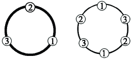
Figure 1: Example of two situations that are indistinguishable by the nodes.

Initially, the state of node $i$ in the first ring is exactly the same as the state of the nodes $j=i,i+m,i+2m,\ldots$ in the second ring. We show by induction that this property must hold at all times $t$. (To keep notation simple, we assume, without any real loss of generality, that $i\neq 1$ and $i\neq m$.)

Indeed, suppose this property holds up to time $t$. At time $t$, node $i$ in the first ring receives a message from node $i-1$ and a message from node $i+1$; and in the second ring, node $j$ satisfying ${j\ (\mbox{mod }m)}=i$ receives one message from $j-1$ and $j+1$. Since ${j-1\ (\mbox{mod }m)}=i-1$ and ${j+1\ (\mbox{mod }m)}=i+1$, the states of $j-1$ and $i-1$ are identical at time $t$, and similarly for and $j+1$ and $i+1$. Thus the messages received by $i$ (in the first ring) and $j$ (in the second ring) at time $t$ are identical. Since $i$ and $j$ were in the same state at time $t$, they must be in the same state at time $t+1$. This proves that they are in the same state forever.

It follows that $y_{i}(t)=y_{j}(t)$ for all $t$, whenever ${j\ (\mbox{mod }m)}=i$, and therefore $f_{m}(x)=f_{km}(x^{k})$. ∎

We can now prove our main negative result, stating that if a family of functions is computable, then the value of the function only depends on the frequencies of the different possible initial values. We define $D=\{(p_{1},\dots,p_{K})\in[0,1]^{K}:\sum_{k=1}^{K}p_{k}=1\}$, which we call the proportion set. We say that a function $h:D\to Y$ corresponds to a family $(f_{n}:{X}^{n}\to Y)$ if for every $x\in{X}^{n}$,

$$f(x_{1},\dots,x_{n})=h\left(p_{1}(x_{1},\ldots,x_{n}),\dots,p_{K}(x_{1},\ldots,x_{n})\right),$$

where

$$p_{k}(x_{1},\ldots,x_{n})=|\{{i}~{}|~{}x_{{i}}={k},\}|/n,$$

so that $p_{k}(x_{1},\ldots,x_{n})$ is the frequency of occurrence of the initial value $k$. In this case, we say that the family $(f_{n})$ is proportion-based.

Theorem 3.1.

Suppose that the family $(f_{n})$ is computable with infinite memory. Then, this family is proportion-based.

Proof.

Let $x$ and $y$ be two sequences of $n$ and $m$ elements, respectively, such that $p_{k}(x_{1},\dots,x_{n})=p_{k}(y_{1},\dots,y_{m})=:\hat{p}_{k}$ for $k=1,\dots,K$, that is, the number of occurrences of $k$ in $x$ and $y$ are $n\hat{p}_{k}$ and $m\hat{p}_{k}$, respectively. Observe that for any $k\in X$, the vectors $x^{m}$ and $y^{n}$ have the same number $mn$ of elements, and both contain $mn\hat{p}_{k}$ occurrences of $k$. The sequences $y^{n}$ and $x^{m}$ can thus be obtained from each other by a permutation, which by Proposition 3.1 implies that $f_{nm}(x^{m})=f_{nm}(y^{n})$. It then follows from Proposition 3.2 that $f_{nm}(x^{m})=f_{n}(x)$ and $f_{mn}(y^{n})=f_{m}(y)$, so that $f_{n}(x)=f_{m}(y)$. This proves that the value of $f_{n}(x)$ is determined by the vector $(p_{1}(x),\dots,p_{n}(x))$. ∎

The following examples illustrate this result.

(a)  The parity function $\sum_{i=1}^{n}x_{i}~{}({\rm mod~{}k})$ is not computable, for any $k>0$.

(b)  In a binary setting $(X=\{0,1\})$, checking whether the number of nodes with $x_{i}=1$ is at least $10$ plus the number of nodes with $x_{i}=0$ is not computable.

(c)  Solitude verification, i.e. checking whether $|i:\{x_{i}=0\}|=1$, is not computable.

(d)  An aggregate difference functions such as $\sum_{i<j}|x_{i}-x_{j}|$ is not computable, even calculated modulo $k$.

4 Reduction of generic functions to the computation of averages

In this section, we show that the computability question for large classes of functions reduces to the computability question for a particular averaging-like function. Namely, we will make use of the following theorem.

Theorem 4.1.

Let $X=\{0,\ldots,K\}$ and define $Y$ to be following set of single-point sets and intervals:

$$Y=\{\{0\},(0,1),\{1\},(1,2),\ldots,\{K-1\},(K-1,K),\{K\}\}$$

(or equivalently, an indexing of this finite collection of intervals). Let $(f_{n})$ be the following family of functions: $f_{n}$ maps $(x_{1},x_{2},\ldots,x_{n})$ to the element of $Y$ which contains the average $\sum_{i}x_{i}/n$. Then, the family $(f_{n})$ is computable.

The proof of Theorem 4.1 is fairly involved and too long to be included in this extended abstract; however, we give an informal description of the algorithm for computing $f_{n}$ in Section 5. In this section, we show that Theorem 4.1 implies the computability of a large class of functions. We will say that a function $h$ on the proportion set is computable if it it corresponds to a proportion-based computable family $(f_{n})$. The level sets of $h$ are defined as the sets $L(y)=\{{p}\in D~{}|~{}h(p)=y\}$, for $y\in Y$.

Theorem 4.2 (Sufficient condition for computability).

Let $h$ be a function from the proportion set $D$ to $Y$. Suppose that every level set $L(y)$ can be written as a finite union,

$$L(y)=\bigcup_{k}C_{i,k},$$

where each $C_{i,k}$ can in turn be written as a finite intersection of linear inequalities of the form

$$\alpha_{1}p_{1}+\alpha_{2}p_{2}+\cdots+\alpha_{K}p_{K}\leq\alpha,$$

or

$$\alpha_{1}p_{1}+\alpha_{2}p_{2}+\cdots+\alpha_{K}p_{K}<\alpha,$$

with rational coefficients $\alpha,\alpha_{1},\ldots,\alpha_{K}$. Then, $h$ is computable.

Proof.

Consider one such linear inequality. Let $P$ be the set of indices $i$ for which $\alpha_{i}\geq 0$. Since all coefficients are rational, we can clear the denominators and rewrite the inequality as

$$\sum_{k\in P}\beta_{k}p_{k}-\sum_{i\in P^{c}}\beta_{k}p_{k}\leq\beta,$$ (4.1)

for nonnegative integers $\beta_{k}$ and $\beta$. Let $\chi_{k}$ be the indicator function associated with initial value $k$, i.e., $\chi_{k}(i)=1$ if $x_{i}=k$, and $\chi_{k}(i)=0$ otherwise, so that $p_{k}=\frac{1}{n}\sum_{i}\chi_{k}(i)$. Then, (4.1), becomes

$$\frac{1}{n}\sum_{i=1}^{n}\left(\sum_{k\in P}\beta_{k}\chi_{k}(i)+\sum_{k\in P^{c}}\beta_{k}(1-\chi_{k}(i))\right)\leq\beta+\sum_{k\in{P^{c}}}\beta_{k},$$

or

$$\frac{1}{n}\sum_{i}q_{i}\leq q^{*},$$

where $q_{i}=\sum_{k\in P}\beta_{k}\chi_{k}(i)+\sum_{k\in P^{c}}\beta_{k}(1-\chi_{k}(i))$ and $q^{*}=\beta+\sum_{k\in P^{c}}\beta_{k}$.

To determine if the latter inequality is satisfied, each node can compute $q_{i}$ and $q^{*}$, and then apply a distributed algorithm that computes $\frac{1}{n}\sum_{i=1}^{n}q_{i}$, which is possible by virtue of Theorem 4.1. To check any finite collection of inequalities, the nodes can perform the computations for each inequality in parallel.

To compute $h$, the nodes simply need to check which set $L(y)$ the frequencies $p_{1},\ldots,p_{K}$ lie in, and this can be done by checking the inequalities defining each $L(y)$. All of these computations can be accomplished with finite automata: indeed, we do nothing more than run finitely many copies of the automata provided by Theorem 4.1, one for each inequality. ∎

Theorem 4.2 shows the computability of functions $h$ whose level-sets can be defined by linear inequalities with rational coefficients. On the other hand, it is clear that not every function $h$ can be computable. (This can be shown by a counting argument: there are uncountably many possible functions $h$, but for the special case of bounded degree graphs, only countably possible algorithms.) Still, the next lemma shows that the set of computable functions is rich enough, in the sense that such functions can approximate any measurable function.

We will call a set of the form $\prod_{{k}=1}^{K}(a_{k},b_{k})$, with every $a_{k},b_{k}$ rational, a rational open box, where $\prod$ stands for Cartesian product. A function that can be written as a finite sum $\sum_{i}a_{i}{1_{B_{i}}}$, where the $B_{i}$ are rational open boxes and the $1_{B_{i}}$ are the associated indicator functions, will be referred to as a box function. Note that box functions are computable by Theorem 4.2.

Corollary 4.3.

If every level set of a function $h:D\to Y$ on the proportion set is Lebesgue measurable, then, for every $\epsilon>0$, there exists a computable box function $h_{\epsilon}:D\to Y$ such that the set $\{h\neq h_{\epsilon}\}$ has measure at most $\epsilon$.

Proof.

The proof relies on the following elementary result from measure theory. Given a Lebesgue measurable set $E\in[0,1]^{K}$ and some $\epsilon>0$, there exists a set $E^{\prime}$ which is a finite union of disjoint open boxes, and which satisfies

$$\mu((E-E^{\prime})\cup(E^{\prime}-E))<\epsilon,$$

where $\mu$ is the Lebesgue measure. By a routine argument, these boxes can be taken to be rational. By applying this fact to the level sets of the function $h$ (assumed measurable), the function $h$ can be approximated by a box function $h_{\epsilon}$. Since box functions are computable, the result follows. ∎

The following corollary states that quantizations of continuous functions are approximable.

Corollary 4.4.

If a function $h:D\to[L,U]\subseteq\Re$ is continuous, then for every $\epsilon>0$ there exists a computable function $h_{\epsilon}:D{\to[L,U]}$ such that $\|h-h_{\epsilon}\|_{\infty}<\epsilon$

Proof.

Since $D$ is compact, $f$ is uniformly continuous. One can therefore partition $D$ into a finite number of subsets $A_{1},A_{2},\dots,A_{q}$, that can be described by linear inequalities with rational coefficients, so that $\max_{p\in A_{j}}h(p)-\min_{p\in A_{j}}h(p)<\epsilon$ holds for all $A_{j}$. The function $h_{\epsilon}$ is then built by assigning to each $A_{j}$ an appropriate value in $\{L,L+\epsilon,L+2\epsilon,\dots,U\}$. ∎

Finally, we show that with infinite memory, it is possible to recover the exact frequencies $p_{k}$. (Note that this is impossible with finite memory, because $n$ is unbounded, and the number of bits needed to represent $p_{k}$ is also unbounded.)

Theorem 4.5.

The vector $(p_{1},\ldots,p_{K})$ is computable with infinite memory.

Proof.

We show that $p_{1}$ is computable exactly, which is sufficient to prove the theorem. Consider the following algorithm, parametrized by a positive integer $m$. The initial set $X_{m}$ will be $\{0,1,\ldots,m\}$ and the output set $Y_{m}$ will be as in Theorem 4.1: $Y_{m}=\{\{0\},(0,1),\{1\},(1,2),\{2\},(2,3),\ldots,\{m-1\},(m-1,m),\{m\}\}$. If $x_{i}=1$, then node sets its initial value $x_{i,m}$ to $m$; else, the node sets its initial value $x_{i,m}$ to $0$. The algorithm computes the function family $(f_{n})$ which maps $X_{m}^{n}$ to the element of $Y_{m}$ containing $(1/n)\sum_{i=1}^{n}x_{i,m}$, which is possible, by Theorem 4.1. We will call this algorithm $Q_{m}$. Let $y_{m}$ be its final output.

The nodes run the algorithms $Q_{m}$ for every positive integer value of $m$, in an interleaved manner. Namely, at each time step, a node runs one step of a particular algorithm $Q_{m}$, according to the following order:

$$Q_{1},\hskip 5.69046ptQ_{1},Q_{2},\hskip 5.69046ptQ_{1},Q_{2},Q_{3},\hskip 5.69046ptQ_{1},Q_{2},Q_{3},Q_{4},\hskip 5.69046ptQ_{1},Q_{2},\ldots$$

At each time $t$, let $m_{i}(t)$ be the smallest $m$ (if it exists) such that the output $y_{i,m}(t)$ of $Q_{m}$ at node $i$ is a singleton (not an interval). We identify this singleton with the numerical value of its single element, and we set $y_{i}(t)=y_{i,m_{i}(t)}(t)/m_{i}(t)$. If $m_{i}(t)$ is undefined, then $y_{i}(t)$ is set to some default value.

It follows from the definition of $Q_{m}$ and from Theorem 4.1 that there exists a time after which the outputs ${y_{i,m}}$ of the algorithms $Q_{1},\dots,Q_{n}$ do not change, and are the same for every node, denoted $y_{m}$. Moreover, at least one of these algorithms has an integer output $y_{m}$. Indeed observe that $Q_{n}$ computes $(1/n)\sum_{i=1}^{n}n1_{x_{i}=1}=\sum_{i=1}^{n}1_{x_{i}=1}$, which is clearly an integer. In particular, $m_{i}(t)$ is eventually well-defined and bounded above by $n$. We conclude that there exists a time after which the output of our overall algorithm is fixed, shared by all nodes, and different from the default value.

We now argue that this value is indeed $p_{1}$. Let $m^{*}$ be the smallest $m$ for which the eventual output of $Q_{m}$ is a single integer $y_{m}$. Note that $y_{m^{*}}$ is the exact average of the $x_{i,m^{*}}$, i.e. $y_{m^{*}}=\frac{1}{n}\sum_{i=1}^{n}m^{*}1_{x_{i}=1}=m^{*}p_{1}$. For large $t$, we have $y_{i}(t)=y_{i,m^{*}}(t)/m^{*}=p_{1}$.

Finally, it remains to argue that the algorithm described here can be implemented with a sequence of automata. All the above algorithm does is run a copy of all the automata implementing $Q_{1},Q_{2},\ldots$ with time-dependent transitions. This can be accomplished with an automaton whose state space is the countable set $\mathcal{N}\times{\cup_{m=1}^{\infty}\prod_{i=1}^{m}{\cal Q}_{i}}$, where ${\cal Q}_{i}$ is the state space of $Q_{i}$, and the set $\mathcal{N}$ of integers is used to keep track of time. ∎

To illustrate the results of this section, let us consider again some examples.

(a)  Majority testing between two options is equivalent to checking whether $p_{1}\leq 1/2$, with alphabet $\{0,1\}$, and is therefore computable.

(b)  Majority testing when some nodes can “abstain” amounts to checking whether $p_{1}-p_{2}\geq 0$, with alphabet $\{0,1,{\rm abstain}\}$. This function family is computable.

(c)  We can ask for the second most popular value out of four, for example. In this case, the sets $A_{i}$ can be decomposed into constituent sets defined by inequalities such as $p_{2}\leq p_{3}\leq p_{4}\leq p_{1}$, each of which obviously has rational coefficients.

(d)  For any subsets $I,I^{\prime}$ of $\{1,\ldots,K\}$, the indicator function of the set where $\sum_{i\in I}p_{i}\geq\sum_{i\in I^{\prime}}p_{i}$ is computable. This is equivalent to checking whether more nodes have a value in $I$ than do in $I^{\prime}$.

(e)  The indicator functions of the sets defined by $p_{1}^{2}\leq 1/2$ and $p_{1}\leq\pi/4$ are measurable, so they are approximable. We are unable to say whether they are computable.

(f)  The indicator function of the set defined by $p_{1}p_{2}\leq 1/8$ is approximable, but we are unable to say whether it is computable.

5 A sketch of the proof of Theorem 4.1

In this section, we sketch an algorithm for computing the average of integer initial values, but omit the proof of correctness. We start with an important subroutine that tracks the maximum (over all nodes) of time-varying inputs at each node.

5.1 Distributed maximum tracking

Suppose that each node $i$ has a time-varying input $u_{i}(t)$ stored in memory at time $t$, belonging to a finite set of numbers ${\cal U}$. We assume that, for each $i$, the sequence $u_{i}(t)$ must eventually stop changing, i.e., that there exists some $T^{\prime}$ such that

$$u_{i}(t)=u_{i}(T^{\prime}),~{}~{}~{}~{}~{}~{}~{}~{}\mbox{ for all }t\geq T^{\prime}.$$

(However, the nodes need not be ever aware that $u_{i}(t)$ has reached its final value.) Our goal is to develop a distributed algorithm whose output eventually settles on the value $\max_{i}u_{i}(T^{\prime})$. More precisely, each node $i$ is to maintain a number $M_{i}(t)$ which must satisfy the following constraint: for every connected graph and any allowed sequences $u_{i}(t)$, there exists some $T^{\prime\prime}$ with

$$M_{i}(t)=\max_{i=1,\ldots,n}u_{i}(t),~{}~{}~{}~{}~{}\mbox{ for all }t\geq T^{\prime\prime}.$$

Moreover, node $i$ must also maintain a pointer $P_{i}(t)$ to a neighbor or to itself. We will use the notation $P^{2}_{i}(t)=P_{P_{i}(t)}(t)$, $P^{3}_{i}(t)=P_{P_{i}^{2}(t)}(t)$, etc. We require the following additional property, for all $t$ larger than $T^{\prime\prime}$: for each node $i$ there exists a node ${j}$ and a power $K$ such that for all $k\geq K$ we have $P^{k}_{i}=j$; moreover, $M_{i}(t)=u_{j}(t)$. In other words, by successively following the pointers $P_{i}(t)$, one can arrive at a node with the maximum value.

Theorem 5.1.

An algorithm satisfying the above conditions exists and can be implemented at each node with a finite automaton whose state can be stored using at most $C(\log|{\cal U}|+d(i))$ bits, for some absolute constant $C$.

We briefly summarize the algorithm guaranteed by this theorem. Each node $i$ initially sets $M_{i}(0)=u_{i}(0),P_{i}(0)=i$. Nodes exchange their values $u_{i}(t)$ and forward the largest value they have seen; every node sets its estimated maximum $M_{i}{(t)}$ equal to that largest value, and sets its pointer $P_{i}$ to the node that forwarded that value to $i$. When some $u_{i}$ changes, the corresponding node sends out a reset message, which is then forwarded by all other nodes. The details of the algorithm and its analysis are somewhat involved because we need to make sure that the reset messages do not cycle forever.

5.2 The averaging algorithm

We continue with an intuitive description of the averaging algorithm. Imagine the initial integer values $x_{i}$ as represented by $x_{i}$ pebbles. Our algorithm attempts to exchange pebbles between nodes with unequal number of pebbles so that the overall distribution becomes more even. Eventually, either all nodes will have the same number of pebbles, or some will have a certain number and others just one more. We let $u_{i}(t)$ be the current number of pebbles at node $i$; in particular, $u_{i}(0)=x_{i}$. An important property of the algorithm is that the total number of pebbles is conserved.

To match nodes with unequal number of pebbles we use the maximum tracking algorithm of Section 5.1. Recall that the algorithm provides nodes with pointers which attempt to track the location of the maximal values. When a node with ${u}_{i}$ pebbles comes to believe in this way that a node with at least $u_{i}+2$ pebbles exists, it sends a request in the direction of the latter node to obtain one or more pebbles. This request follows a path to a node with a maximal number of pebbles, until the request either gets denied, or gets accepted by a node with at least $u_{i}+2$ pebbles.

More formally, the algorithm uses two types of messages:

1. (Request, $r$): This is a request for a transfer of value. Here, $r$ is an integer that represents the current number of pebbles at the emitter.

2. (Accept, $w$): This corresponds to acceptance of a request, and subsequent transfer of $w$ pebbles to the requesting node. A request with a value $w=0$ represents a request denial.

As part of the algorithm, the nodes run the maximum tracking algorithm of Section 5.1, as well as a minimum tracking counterpart. In particular, each node $i$ has access to the variables $M_{i}(t)$ and $P_{i}(t)$ of the maximum tracking algorithm (recall that these are, respectively, the estimated maximum and a pointer to a neighbor). Furthermore, each node maintains three additional variables.

• “mode”$\in$ {free,blocked}. Initially, the mode of every node is free. Nodes become blocked when they are handling requests.

• “$Rin_{i}(t)$”, “$Rout_{i}(t)$” are pointers to a neighbor of $i$ or to itself. They represent, respectively, the node from which $i$ has received a request, and the node to which $i$ has transmitted a request. Initially, $Rin_{i}(0)=Rout_{i}(0)=\emptyset.$

The algorithm is described in Figure 2.

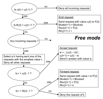
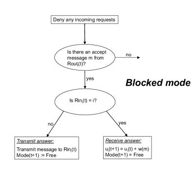
Figure 2: Representation of the average computation algorithm

A key step in the proof of Theorem 4.1 is the following proposition, whose proof is omitted.

Proposition 5.1.

There is a time $t^{\prime}$ such that ${u}_{i}(t)={u}_{i}(t^{\prime})$, for all $i$ and $t\geq t^{\prime}$. Moreover,

$$\sum_{i}u_{i}(t^{\prime}) = \sum_{i}u_{i}(0)\ {=\ \sum_{i}x_{i},}$$

$$|u_{i}({t^{\prime}})-u_{j}({t^{\prime}})| \leq 1,\mbox{ for all }i,j.$$

We now conclude our sketch of the proof of Theorem 4.1. Let $u_{i}^{*}$ be the value that $u_{i}(t)$ settles on. It follows from Proposition 5.1 that if the average $\bar{x}$ of the inputs $x_{i}$ is integer, then $u_{i}(t)=u_{i}^{*}=\bar{x}$ will eventually hold for every $i$. If $\bar{x}$ is not an integer, then some node will eventually have ${u_{i}^{*}}=\lfloor\bar{x}\rfloor$ and others $u_{i}^{*}=\lceil\bar{x}\rceil$. Using the maximum and minimum computation algorithm, nodes will eventually have a correct estimate of $\max_{i}u_{i}^{*}$ and $\min_{i}u_{i}^{*}$, because each $u_{i}(t)$ converges to $u_{i}^{*}$. This allows the nodes to determine if the average is exactly $\bar{x}$ (integer average), or if it lies in $(\bar{u}_{i}^{*},\bar{u}^{*}_{i}+1)$, or $(\bar{u}^{*}_{i}-1,\bar{u}^{*}_{i})$, which is the property asserted by Theorem 4.1.

References

- [1] “Local and global properties in networks of processors,” D. Angluin, Proceedings of the twelfth annual ACM symposium on Theory of computing, 1980.
- [2] “An introduction to population protocols,” J. Aspnes and E. Ruppert, Bulletin of the European Association for Theoretical Computer Science, 93:98 117, October 2007.
- [3] “Distributed Average Consensus using Probabilistic Quantization,” T.C. Aysal, M. Coates, M. Rabbat, 14th IEEE/SP Workshop on Statistical Signal Processing, 2007.
- [4] Y. Afek and Y. Matias, “Elections in anonymous networks,” Information and Computation, 113:2, pp. 113-330, 1994.
- [5] O. Ayaso, D. Shah, M. Dahleh, “Counting bits for distributed function computation,” Proceedings of the IEEE International Symposium on Information Theory, 2008.
- [6] H. Attiya, M. Snir, M.K. Warmuth, “Computing on an anonymous ring,” Journal of the ACM, Vol. 35, No. 4, pp. 845 - 875, 1988.
- [7] F. Bénézit, P. Thiran, M. Vetterli“Interval consensus: from quantized gossip to voting,” , Proceedings of ICASSP 08.
- [8] R. Carli, F. Bullo, “Quantized Coordination Algorithms for Rendezvous and Deployment, ” preprint.
- [9] P. Frasca, R. Carli, F. Fagnani, S. Zampieri, “Average consensus on networks with quantized communication,” preprint.
- [10] F. Fich, E. Ruppert, “Hundreds of impossibility results for distributed computing,” Distributed Computing, Vol. 16, pp. 121-163, 2003.
- [11] A. Giridhar, P.R. Kumar, “Computing and communicating functions over sensor networks,” IEEE Journal on on Selected Areas in Communications, Vol. 23, No. 4, pp. 755- 764, 2005.
- [12] P. Gacs, G.L. Kurdyumov, L.A. Levin, “One-dimensional uniform arrays that wash out finite islands,” Problemy Peredachi Informatsii, 1978.
- [13] A.G. Greenberg, P. Flajolet, R. Lander, “Estimating the multiplicity of conflicts to speed their resolution in multiple access channels,” Journal of the ACM, Vol 34, No. 2, 1987.
- [14] Y. Hassin and D. Peleg, “Distributed Probabilistic Polling and Applications to Proportionate Agreement,” Information and Computation 171, (2001), 248-268.
- [15] A. Jadbabaie, J. Lin, A.S. Morse, “ Coordination of groups of mobile autonomous agents using nearest neighbor rules,” IEEE Transactions on Automatic Control, Vol. 48, No. 6, pp. 988-1001, 2003.
- [16] A. Kashyap, T. Basar, R. Srikant, “Quantized consensus,” Automatica, Vol. 43, No. 7, pp. 1192-1203, 2007.
- [17] E. Kranakis, D. Krizanc, J. van den Berg, “Computing boolean functions on anonymous networks,” Proceedings of the 17th International Colloquium on Automata, Languages and Programming, Warwick University, England, July 16 20, 1990.
- [18] N. Khude, A. Kumar, A. Karnik, “Time and energy complexity of distributed computation in wireless sensor networks,” Proceedings of INFOCOM 05.
- [19] N. Katenka, E. Levina, and G. Michailidis, “Local Vote Decision Fusion for Target Detection in Wireless Sensor Networks,” IEEE Transactions on Signal Processing, 56(1):329-338, 2008.
- [20] S. Kar, J.M Moura, “Distributed average consensus in sensor networks with quantized inter-sensor communication, ” IEEE International Conference on Acoustics, Speech and Signal Processing, 2008.
- [21] M. Land, R.K. Belew, “No perfect two-state cellular automaton for density classification exists, ” Physical Review Letters, vol 74, no. 25, pp. 5148-5150, Jun 1995.
- [22] Y. Lei, R. Srikant, G.E. Dullerud, “Distributed Symmetric Function Computation in Noisy Wireless Sensor Networks,” IEEE Transactions on Information Theory, Vol. 53, No. 12, pp. 4826-4833, 2007.
- [23] L. Liss, Y. Birk, R. Wolff, and A. Schuster, “A Local Algorithm for Ad Hoc Majority Voting Via Charge Fusion,” Proceedings of DISC’04, Amsterdam, the Netherlands, October, 2004
- [24] S. Martinez, F. Bullo, J. Cortes, E. Frazzoli, “On synchronous robotic networks - part I: models, tasks, complexity,” IEEE Transactions on Robotics and Automation, Vol. 52, No. 12, pp. 2199 - 2213, 2007.
- [25] S. Mukherjeea, H. Kargupta, “Distributed probabilistic inferencing in sensor networks using variational approximation,” Journal of Parallel and Distributed Computing, Volume 68, Issue 1, Pages 78-92, 2008.
- [26] S. Moran, M.K. Warmuth, “Gap Theorems for Distributed Computation,” SIAM Journal of Computing Vol. 22, No. 2, pp. 379-394 (1993).
- [27] A. Nedic, A. Olshevsky, A. Ozdaglar, J.N. Tsitsiklis, “On distributed averaging algorithms and quantization effects,” preprint, to be published in Proceedings of 47th IEEE Conference on Decision and Control, 2008.
- [28] D. Peleg, “Local majorities, coalitions and monopolies in graphs: a review, ” Theoretical Computer Science, Vol. 282, No. 2, pp. 231-237, 2002.
- [29] E. Perron, D. Vasuvedan, M. Vojnovic, “Using Three States for Binary Consensus on Complete Graphs,” preprint.
- [30] L. Xiao and S. Boyd, “Fast Linear Iterations for Distributed Averaging,” Systems and Control Letters, 53:65-78, 2004.
- [31] M. Yamashita and T. Kameda, “Computing on an anonymous network,” Proceedings of the seventh annual ACM Symposium on Principles of distributed computing, 1988.