Untangling the Braid:
Finding Outliers in a Set of Streams

Abstract

Monitoring the performance of large shared computing systems such as the cloud computing infrastructure raises many challenging algorithmic problems. One common problem is to track users with the largest deviation from the norm (outliers), for some measure of performance. Taking a stream-computing perspective, we can think of each user’s performance profile as a stream of numbers (such as response times), and the aggregate performance profile of the shared infrastructure as a “braid” of these intermixed streams. The monitoring system’s goal then is to untangle this braid sufficiently to track the top $k$ outliers. This paper investigates the space complexity of one-pass algorithms for approximating outliers of this kind, proves lower bounds using multi-party communication complexity, and proposes small-memory heuristic algorithms. On one hand, stream outliers are easily tracked for simple measures, such as max or min, but our theoretical results rule out even good approximations for most of the natural measures such as average, median, or the quantiles. On the other hand, we show through simulation that our proposed heuristics perform quite well for a variety of synthetic data.

1 Introduction

Imagine a general purpose stream monitoring system faced with the task of detecting misbehaving streams among a large number of distinct data streams. For instance, a network diagnostic program at an IP router may wish to highlight flows whose packets experience unusually large average network latency. Or, a cloud computing service such as Yahoo Mail or Amazon’s Simple Storage Service (S3), catering to a large number of distinct users, may wish to track the quality of service experienced by its users. The performance monitoring of large, shared infrastructures, such as cloud computing, provides a compelling backdrop for our research, so let us dwell on it briefly. An important characteristics of cloud computing applications is the sheer scale and large number of users: Yahoo Mail and Hotmail support more than 250 million users, with each user having several GBs of storage. With this scale, any downtime or performance degradation affects many users: even a guarantee of $99.9\%$ availability (the published numbers for Google Apps, including Gmail) leaves open the possibility of a large number of users suffering downtime or performance degradation. In other words, even a $0.1\%$ user downtime affects 250,000 users, and translates to significant loss of productivity among users. Managing and monitoring systems of this scale presents many algorithmic challenges, including the one we focus on: in the multitude of users, track those receiving the worst service.

Taking a stream-computing perspective, we can think of each user’s performance profile as a stream of numbers (such as response times), and the aggregate performance profile of the whole infrastructure as a braid of these intermixed streams. The monitoring system’s goal then is to untangle this braid sufficiently to track the top $k$ outliers. In this paper, we study questions motivated by this general setting, such as “which stream has the highest average latency?”, or “what is the median latency of the $k$ worst streams?,” “how many streams have their $95$th percentile latency less than a given value?” and so on.

These problems seem to require peering into individual streams more deeply than typically studied in most of the extant literature. In particular, while problems such as heavy hitters and quantiles also aim to understand the statistical properties of IP traffic or latency distributions of webservers, they do so at an aggregate level: heavy hitters attempt to isolate flows that have large total mass, or users whose total response time is cumulatively large. In our context, this may be uninteresting because a user can accumulate large total response time because he sends a lot of requests, even though each request is satisfied quickly. On the other hand, streams that consistently show high latency are a cause for alarm. More generally, we wish to isolate flows or users whose service response is bad at a finer level, perhaps taking into account the entire distribution.

1.1 Problem Formulation

We have a set ${\cal B}$, which we call a braid, of $m$ streams $\{{S}_{1},{S}_{2},\ldots,{S}_{m}\}$, where the $i$th stream has size $n_{i}$, namely, $n_{i}=|{S}_{i}|$. We assume that the number of streams is large and each stream contains potentially an unbounded number of items; that is, $m\gg 1$ and $n_{i}\gg 1$, for all $i$. By $v_{ij}$, we will mean the value of the $j$th item in the stream ${S}_{i}$; we make no assumptions about $v_{ij}$ beyond that they are real-valued. In the examples mentioned above, $v_{ij}$ represents the latency of the $j$th request by the $i$th user. We formalize the misbehavior quality of a stream by an abstract weight function ${\lambda}$, which is function of the set of values in the stream. For instance, ${\lambda}({S})$ may denote the average or a particular quantile of the stream ${S}$. Our goal is to design streaming algorithms that can estimate certain fundamental statistics of the set $\{{\lambda}({S}_{1}),{\lambda}({S}_{2}),\ldots,{\lambda}({S}_{m})\}$.

When needed, we use a self-descriptive superscript to discuss specific weight functions, such as ${\lambda}^{\rm avg}$ for average, ${\lambda}^{\rm med}$ for median, ${\lambda}^{\max}$ for maximum, ${\lambda}^{\min}$ for minimum etc. For instance, if we choose the weight to be the average, then ${\lambda}^{\rm avg}({S})$ denotes the average value in stream ${S}$, and

$$\max\{{\lambda}^{\rm avg}({S}_{1}),{\lambda}^{\rm avg}({S}_{2}),\ldots,{\lambda}^{\rm avg}({S}_{m})\}$$

computes the worst-stream by average latency. Throughout we will focus on the one-pass model of data streams.

As is commonly the case with data stream algorithms, we must content ourselves with approximate weight statistics because even in the single stream setting neither quantiles nor frequent items can be computed exactly. With this in mind, let us now precisely define what we mean by a guaranteed-quality approximation of high weight streams. There are two natural and commonly used ways to quantify an approximation: by rank or by value. (Recall that the rank of an element $x$ in a set is the number of items with value equal to or less than $x$.)

• Rank Approximation: Let ${\lambda}$ be an arbitrary weight function (e.g. median), and let ${\lambda}_{i}={\lambda}({S}_{i})$ be the value of this function for stream ${S}_{i}$. We say that a value ${\lambda}^{\prime}_{i}$ is a rank approximation of ${\lambda}_{i}$ with error $E$ if the rank of ${\lambda}^{\prime}_{i}$ in the stream ${S}_{i}$ is within $E$ of the rank of ${\lambda}_{i}$. Namely,

  $$|{\rm rank}({\lambda}^{\prime}_{i},{S}_{i})\;-\;{\rm rank}({\lambda}_{i},{S}_{i})|\>\leq\>E,$$

  where ${\rm rank}(x,{S})$ denotes the rank of element $x$ in stream ${S}$ and $E$ is a non-negative integer. Thus, if we are estimating the median latency of a stream, then ${\lambda}^{\prime}_{i}$ is its rank approximation with error $E$ if —rank (λ’_i,S _i )  -  ⌊—S_i—/2 ⌋—  ≤  E .

• Value Approximation: Let ${\lambda}$ be an arbitrary weight function (e.g. median), and let ${\lambda}_{i}={\lambda}({S}_{i})$ be the value of this function for stream ${S}_{i}$. We say that ${\lambda}^{\prime}_{i}$ is a value approximation of ${\lambda}_{i}$ with relative error $c$ if

  $$|{\lambda}^{\prime}_{i}\;-\;{\lambda}_{i}|\>\leq\>c{\lambda}_{i}.$$

While rank approximation often seems more appropriate for quantile-based weights, and value approximation for average, they both yield useful insights into the underlying distribution. For instance, given any positive $\alpha$, at most $|{S}|/\alpha$ items in ${S}$ can have value more than $\alpha{\lambda}^{\rm avg}({S})$. Thus, a rank approximation of ${\lambda}^{\rm avg}({S})$ also localizes the relative position of the approximation. Conversely, a value approximation of the median or quantile can be especially useful when the distribution is highly clustered, making the rank approximation rather volatile—two items may differ greatly in rank, but still have values very close to each other. Our overall goal is to estimate streams with large weights with guaranteed quality of approximation: in other words, if we assert that the worst stream in the set ${\cal B}$ has median weight ${\lambda}^{*}$ then we wish to guarantee that ${\lambda}^{*}$ is an approximation of $\max\{{\lambda}^{\rm med}({S}_{1}),{\lambda}^{\rm med}({S}_{2}),\ldots,{\lambda}^{\rm med}({S}_{m})\}$, either by rank or by value. We prove possibility and impossibility results on what error bounds are achievable with small memory.

1.2 Our Contributions

We begin with a simple observation that finding the top k streams under the ${\lambda}^{max}$ or ${\lambda}^{min}$ weight functions is easy: this can be done using $O(k)$ space and $O(\log k)$ per-item processing time. In the context of webservices monitoring applications, this allows us to track the $k$ streams with worst latency values. As is well known, however, statistics based on max or min values are highly volatile due to outlier effects, and filtering based on more robust weight functions such as quantiles or even average is preferred.

We propose a generic scheme that can estimate the weight of any stream using $O(\varepsilon^{-2}\log U\log\delta^{-1})$ space (being $U$ the size of the range of the values in the streams), with rank error $\varepsilon\sum_{i=1}^{m}n_{i}$ with probability at least $1-\delta$. With this, we can report the weights of the top $k$ streams for any of the natural functions such as average, median, or other quantiles so that the rank error in the reported values is at most $\varepsilon\sum_{i=1}^{m}n_{i}$.

One may object to the $\sum_{i=1}^{m}n_{i}$ term in the rank approximation, and ask for a more desirable $\varepsilon n_{i}$ error term so that the error depends only on the size of an individual stream, rather than the whole set of streams. On pragmatic terms also, this is justified because even for modest values (a few thousand streams, each with a million or so items), the $\sum_{i=1}^{m}n_{i}$ error can make the approximation guarantee worthless. In essense, our error approximation is linearly worsening with the number of streams, which is not a very scalable use of space.

Unfortunately, we prove an impossibility result showing that achieving $\varepsilon n_{i}$ error in rank approximation requires space at least linear in the number of streams (the braid size). Worse yet, our lower bound even rules out $\varepsilon\tilde{n}$ rank approximation, where $\tilde{n}$ is the average stream size in the set. Thus, the space complexity is not an artifact of rarity, as is the case with the frequent item problem. In particular, we show that even if all streams in the braid have size $\Theta(\tilde{n})$, achieving rank approximation $\varepsilon\tilde{n}$ requires space $\Omega(m(\frac{1-2\varepsilon}{1+2\varepsilon})^{2+\gamma})$, for any $\gamma>0$, where $m$ is the number of streams in the braid.

Similarly, for the value approximation we show that estimating the average latency of the worst stream in ${\cal B}$ within a factor $t$ requires $\Omega(m/t^{2+\gamma})$ space. Our lower bounds also rule out optimistic bounds even for highly structured and special-case streams. For instance, consider a round robin setting where values arrive in a round-robin order over the streams, so at any instant the size of any two streams differs by at most one. One may have hoped that for such highly structured streams, improved error estimates should be possible. Unfortunately, a variant of our main construction rules out that possibility as well.

In the face of these lowers bounds, we designed and implemented two algorithms, ExponentialBucket and VariableBucket, and evaluated them for a variety of synthetic data distributions. We use three quality metrics to evaluate the effectiveness of our schemes: precision and recall, which measures how many of the top $k$ captured by our scheme are true top $k$, distortion, which measures the average rank error of the captured streams relative to the true top $k$, and average value error, which measures absolute value differences. We tested our scheme on a variety of synthetic data distributions. These data use a normal distribution of values within the streams, and either a uniform or a normal distribution across streams. In all these cases, our precision approaches 100% for all three metrics (average, median, 95th percentile), the distortion is between 1 and 2, and the average error is less than $0.02$. The memory usage plot also confirms the theory that the size of the data structure remains unaffected by the number and the sizes of the streams.

1.3 Related Work

Estimation of stream statistics in the one-pass model has received a great deal of interest within the database, networking, theory, and algorithms communities. While the one-pass majority finding algorithm dates back to Misra and Gries [14], and tradeoffs between memory and the number of passes required goes back to the work of Munro and Paterson [15], a systematic study of the stream model seems to have begun with the influential paper of Alon, Matias and Szegedy [1], who showed several striking results, including space lower bounds for estimating frequency moments, as well as for determining the frequency of the most frequent item in a single stream. While some statistics such as the average, min, and the max can be computed exactly and space-efficiently, other more holistic statistics such as quantiles cannot. Fortunately, however, several methods have been proposed over the last decade to approximate these values with bounded error guarantees. For instance, quantiles can be estimated with additive error $\varepsilon n$ using space $O(\varepsilon^{-1}\log n)$ [9] or space $O(\varepsilon^{-1}\log U)$ [18] where $n$ is the stream size and $U$ is the largest integer value for the stream items. There is also a rich body of literature on finding frequent items, top $k$ items, and heavy hitters [5, 4, 10, 12, 13, 17].

Schemes such as Counting Bloom filters [8] or Count-Min sketches [6] can be viewed as methods for estimating statistics over multiple streams. In particular, these methods are motivated by the need to estimate the sizes of large flows at a router: in our terminology, these methods estimate the aggregate sizes of the top $k$ streams in the braid. By contrast, we are interested in more refined statistics (e.g. top $k$ by the average value) that require peering into the streams, rather than simply aggregating them. Bonomi et al. [3] have extended Bloom filters to maintain not just the presence or absence of a stream, but also some state information about the stream. But this state information does not reflect any aggregate statistical properties of the stream itself.

The time-series data mining community has focused on finding similar [7] or dissimilar sequences [11] in a set of large time-series sequences. But this work is not geared towards a one-pass stream setting and hence assumes that we have $O(m)$ memory available where $m$ is the number of streams.

1.4 Organization

Our paper is organized in five sections. In Section 2, we present our main theoretical results, namely, the lower bounds on the space complexity of single-pass algorithms for detecting outlier streams in a braid. In Section 3, we propose two generic space-efficient schemes for estimating the top $k$ streams in a braid, and analyze their error guarantees. In Section 4, we discuss our experimental results. Finally, we conclude with a discussion in Section 5.

2 Space Complexity Lower Bounds

In this section, we present our main theoretical results, namely, space complexity lower bounds that rule out space-efficient approximation of outlier streams in a fairly broad setting. We mentioned earlier that for simple weight functions such as the max or min, one can easily track the top $k$ streams, using just $O(k)$ space and $O(\log k)$ per-item processing. (This is easily done by maintaining a heap of $k$ distinct streams with the largest item values.) Surprisingly, this good news ends rather abruptly: we show that even tracking top $k$ streams using the second largest item is already hard, and requires memory proportional to the size of the braid, $|{\cal B}|$. Similarly, we argue that while tracking streams with the maximum or the minimum items is easy, tracking streams with the largest spread, namely, difference of the maximum and the minimum items, requires linear space. Our main result rules out even good approximation of most of the major statistical measures, such as average, median, quantiles, etc.

We begin by recalling our formal definition of approximating the outlier streams. Suppose we wish to rank the streams in the braid ${\cal B}$ using a weight function ${\lambda}$. Without loss of generality, assume that the top $k$ streams are indexed $1,2,\ldots,k$; that is, ${\lambda}_{1}\geq{\lambda}_{2}\geq\cdots\geq{\lambda}_{k}$. We say that a stream $S_{i}$ is approximately a top $k$ stream if its ${\lambda}$-value is at least as large as ${\lambda}_{k}$ within the approximation error range. For instance, suppose we are using the median latency ${\lambda}^{\rm med}$, then stream $S_{i}$ is a top $k$ stream with rank approximation $E$ if the value of item with rank $|S_{i}|/2+E$ (true median plus the rank error) in $S_{i}$ is at least as large as ${\lambda}_{k}$. Similarly, one can define the approximation for value approximation. In the following, we discuss our lower bounds, which are all based on the multi-party communication complexity [2, 19, 16]. All our lower bounds employ variations on a single construction, so we begin by describing this general argument below.

2.1 The Lower Bound Framework

Our lower bounds are based on reductions from the multi-party set-disjointness problem, which is a well-known problem in communication complexity [16]. An instance DISJ_m,t of the multi-party set disjointness problem consists of $t$ players and a set of items $A=\{1,2,\ldots,m\}$. The player $i$, for $i=1,2,\ldots,t$, holds a subset $A_{i}\subseteq A$. Each instance comes with a promise: either all the subsets $A_{1},A_{2},\ldots A_{t}$ are pairwise disjoint, or they all share a single common element but are otherwise disjoint. The former is called the YES instance (disjoint sets), and the latter is called the NO instance (non-disjoint sets). The goal of a communication protocol is to decide whether a given instance is a YES instance or a NO instance. The protocol only counts the total number of bits that are exchanged among the players in order to decide this; the computation is free. We will use the following result from communication complexity [2]: any one-way protocol (where player $i$ sends a message to player $i+1$, for $i=1,2,\ldots,t$, that decides between all YES instances and NO instance with success probability greater than $1-\delta$, for any $0<\delta<1$, requires at least $\Omega(m/t^{1+\gamma})$ bits of communication, where recall that $t$ is the number of players and $m$ is the size of the set and $\gamma>0$ is an arbitrarily small constant.

The idea behind our lower bound argument is to simulate a one-way multi-party set-disjointness protocol using a streaming algorithm for the top $k$ streams. If the streaming algorithm uses a synopsis data structure of size $M$, then we show that there is a one-way protocol using $O(Mt)$ bits that can solve the $t$-party disjointness problem. Because the latter is known to have a lower bound of $\Omega(m/t^{1+\gamma})$, it implies that the memory footprint of the streaming algorithm becomes $\Omega(m/t^{2+\gamma})$. The basic construction associates a stream with each element of the set $A$; namely, the stream $S_{i}$ is identified with the item $i\in A$. See Fig. 1 for an example. We initialize each stream with some values, and then insert the remaining values based on the sets $A_{i}$ held by the $t$ players; these values depend on specific constructions. The key idea behind all our constructions is that the braid of streams is such that approximating the top $k$ streams within the approximation range requires distinguishing between the YES and NO instances of the underlying set-disjoint problem. We present the details below as we discuss specific constructions. We begin with our main result on the space complexity of tracking the top $k$ streams under the most common statistical measures, such as median, quantile, or average.

2.2 Space Complexity of Ranking by Median or Average

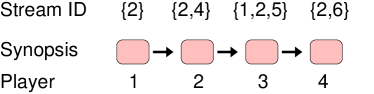
Figure 1: Illustration of a NO instance of DISJ_6,4, with four players. The subsets of the players are shown above their ids, and the values inserted by them into the streams (following the protocol of Theorem 1) are shown in the Table 1

.

Stream ID	1	2	3	4	5	6
Player 1	0	1	0	0	0	0
Player 2	0	1	0	1	0	0
Player 3	1	1	0	0	1	0
Player 4	0	1	0	0	0	1

Table 1: The values inserted by the players of Figure 1 in the lower bound construction of Theorem 1 are shown in this table.

Theorem 1

Let ${\cal B}$ be a braid of $m$ streams, where each stream has $\Theta(n)$ elements. Then, determining the top stream in ${\cal B}$ by median value, within rank error $\varepsilon n$ ($0<\varepsilon<1/2$) requires space at least Ω(m(1-2ε1+2ε)^2+γ). for arbitrarily small $\gamma>0$. That is, finding the stream with the maximum median latency, within additive rank approximation error $\varepsilon n$, requires essentially space linear in the number of streams.

Proof 2.2.

Suppose there exists a stream synopsis of size $M$ that can estimate the latency of the maximum median latency stream within rank error $\varepsilon n$. We now show a reduction that can use this synopsis to solve the multi-party set disjointness problem using $O(M)$ bits of communication. Let $p$ be an integer, to be fixed later. We initialize the synopsis by inserting $p$ items in each stream with value 0. The multi-party protocol then modifies the stream as follows, one player at a time, from player 1 through $t$. On his turn, if player $j$ has item $i$ in its set, then it inserts $p$ items of value 1 in stream $i$, for each $i\in A_{j}$. If the player $j$ does not have item $i$ in its set, then it inserts $p$ items of value $0$ in the stream $i$. (Recall that items of the ground set $A$ correspond to streams in our construction.) Thus each player inserts precisely $pm$ values to the streams, and in the end, each stream has exactly $p+pt$ items in it. An example of the running of this protocol is shown in Fig. 1 and the corresponding values inserted by each player is tabulated in Table 1.

Figure 2: Distribution of values in streams for YES and NO instances of DISJ_m,t. For the YES instance, the median value is 0 up to a rank error of $pt-p(t+1)/2$, while for the NO instance, the median value is 1 up to a rank error of $p(t+1)/2-p$.

After all the $t$ players are done, we output YES if the maximum median latency among all streams is 0, and otherwise we return NO. We now reason why this helps decide the set-disjointness problem. Suppose the instance on which we ran the protocol is a YES instance. Then any stream has either all 0 values (this happens when index corresponding to this stream is absent from all sets $A_{j}$), or it has $p$ values equal to $1$ and $pt$ values equal to $0$ (because of the disjointness promise, the index corresponding to this stream occurs in precisely one set $A_{j}$ and that $j$ inserts $p$ copies of $1$ to this stream, while others insert $0$s). See Fig. 2. Therefore up to a rank error $p(t-1)/2$ the median latency of all the streams is 0. On the other hand, if this is a NO instance, then there exists a stream that has $p$ 0 values and $pt$ values equal to $1$. This stream, therefore, has a median latency of $1$ up to a rank error $p(t-1)/2$. Therefore our algorithm can distinguish between a YES and a NO instance.

We may choose $p=n/(1+t)$, so that each stream has size $n$ and our rank error is $n\frac{1}{2}\frac{t-1}{t+1}$. Since the algorithm uses $O(M)$ space and there are $t$ players, the total communication complexity is $\Theta(Mt)$, which by the communication complexity theorem is $\Omega(m/t^{1+\gamma})$. Finally, solving the equality $\varepsilon=\frac{1}{2}\frac{t-1}{t+1}$ for $t$, we get the desired lower bound that $M=\Omega\left(m\left(\frac{1-2\varepsilon}{1+2\varepsilon}\right)^{2+\gamma}\right)$. This completes the proof.

We point out that our stream construction is highly structured, meaning that this lower bound rules out good approximation even for very regular and balanced streams. In particular, the difficulty of estimating the maximum median latency is not a result of rarity of the target stream: indeed, all streams have equal size. Moreover, the construction can be implemented in a way so that items are inserted into the streams in a round-robin way (see Table 1). Therefore, the construction is also not dependent on a pathological spikes in stream population. Thus, even under very strict ordering of values in the streams, the problem of determining high weight streams remains hard.

It is easy to see that the construction is easily modified to prove similar lower bounds for other quantiles. The same construction also shows a space lower bound for determining the maximum average latency stream. Simply observe that the average latency for the NO instance is $1/(1+t)$, while the average latency for the YES instance is $t/(1+t)$. Therefore any $t$-approximation algorithm for the average measure requires space at least $\Omega(m/t^{2+\gamma})$, for any $t\geq 2$ and $\gamma>0$.

Theorem 2.3.

Determining the top stream by average value within relative error at most $t$ requires at least $\Omega(m/t^{2+\gamma})$ space, where $m$ is the number of streams in the braid, $t\geq 2$ and $\gamma>0$.

2.3 Lower Bound for Second Largest

Surprisingly, similar constructions also show that even minor variations of the easy case (finding the stream with the largest or the smallest extremal value) make the problem provably hard. In particular, suppose we want to track the stream with the maximum second largest value. Let us denote this weight function as ${\lambda}^{2max}$. Our proof below proves a space lower bound for even approximating this. In particular, we say that an streaming algorithm finds the second largest-valued stream with approximation factor $c$ if it returns a stream whose rank by the second largest value is at most $2c$, for any integer $c\geq 1$. Note that this definition of approximation is one sided, because the approximate value returned always has rank $2c\geq 2$. (Of course, allowing $c<1$ trivializes the problem because then we can always use the max value instead of the second largest.) Then, we have the following.

Theorem 2.4.

Determining the top stream by second-largest value within approximation factor $t$ requires at least $\Omega(m/t^{2+\gamma})$ space, for any $\gamma>0$, where $m$ is the number of streams in the braid and $t\geq 2$ is an integer.

Proof 2.5.

In this case, suppose there exists a streaming algorithm for the top stream by second largest value problem using space $M$, and consider the following reduction from an instance of the $t$-party set-disjointness problem. Each player $j$, for $j=1,2,\ldots,t$, in turn adds items to stream using the following rule: player $j$ inserts values $j+1$ and $1/(j+1)$ in the stream $S_{i}$ for each $i$ in its set $A_{j}$. For all other streams that it does not hold, it inserts two 0 values in that stream. Therefore every player inserts $2m$ values into the braid and at the end of the protocol, each stream has exactly $2t$ values.

At the end, we return YES to the set-disjointness problem if our streaming algorithm computes the value of the top stream as less than 1, and NO otherwise. We now reason its correctness. If the $t$-party instance is a YES instance, then any stream $i$ either contains the values 0, or it contains values $0,p+1$ and $1/(p+1)$, for some $1\leq p\leq t$. Thus, the top stream by the second largest value has value less than 1 up to an approximation factor of $t/2$. On the other hand, if this is a NO instance, then there exists a stream that includes all the values $1/(t+1),1/t,\ldots,t,t+1$, whose second largest value is $t$. Therefore if our algorithm has an approximation ratio better than $t/2$, it can distinguish between YES and NO instances. Because our protocol requires sending $M$-size synopsis to $t$ players, the total communication complexity is $\Theta(Mt)$, which by the lower bound on set-disjointness is at least $\Omega(m/t^{1+\gamma})$. Therefore, determining the top stream by second largest must require at least $\Omega(m/t^{2+\gamma})$ space, and this completes the proof.

2.4 Lower Bound for Spread

We next argue that while tracking the top stream with the largest or the smallest value is possible, tracking the top stream with the largest spread, namely, $\max(S)-\min(S)$ is not possible without linear space.

Theorem 2.6.

Determining the top stream by the spread requires at least $\Omega(m)$ space, where $m$ is the number of streams in the braid.

Proof 2.7.

Let us consider an instance of DISJ_m,t and a streaming algorithm with a synopsis of size $M$ which can determine the stream with maximum spread.

In this case, we can use a 2-party set-disjointness lower bound. Let us call the two players, ODD and EVEN. We begin by inserting a single value 0 in each of the $m$ streams. First, the ODD player inserts the value $-1$ into each stream $S_{i}$ for which $i$ is in its set $A_{\textrm{ODD}}$. Next, the EVEN player inserts the value $+1$ into each stream $S_{i}$ for which $i$ is in its set $A_{\textrm{EVEN}}$. Clearly, the top stream by the maximum spread has spread 1, then the sets of ODD and EVEN are disjoint, and so this is a YES instance. Otherwise, the top stream has spread 2, and this is a NO instance. The synopsis size of the streaming algorithm, therefore, is at least $\Omega(m)$. This completes the proof.

This finishes the discussion of our lower bounds. The main conclusion is that approximating the top $k$ streams either by average value, within any fixed relative error, or by any quantile, within a rank approximation error of $\varepsilon n_{i}$, is not possible, where $n_{i}$ is the size of the top stream. In fact, the lower bound even rules out the rank approximation within error of $\varepsilon\tilde{n}$, where $\tilde{n}$ is the average size of the streams in the braid.

In the following section, we complement these lower bounds by describing a scheme with a worst-case rank approximation error $\sum_{i=1}^{m}\varepsilon n_{i}$, using roughly $O(\varepsilon^{-2}\log U)$ space.

3 Algorithms for Braid Outliers

We begin with a generic scheme for estimating top $k$ streams, and then refine it to get the desired error bounds. The basic idea is simple. Without loss of generality, suppose the items (values) in the streams come from a range $[1,U]$. We subdivide this range into subranges, called buckets, that are pairwise disjoint and cover the entire range $[1,U]$. All stream entries with a value $v$ are mapped to the bucket that contains $v$. Within the bucket, we use a sketch, such as the Count-Min sketch, to keep track of the number of items belonging to different streams. With this data structure, given any value $v$ and a stream index $i$, we can estimate how many items of stream $S_{i}$ have values in the range $[1,v]$. This is sufficient to estimate various streams statistics such as quantiles and the average. We point that this estimation incurs two kinds of error: one, a sketch has an inherent error in estimating how many of the items in a bucket belong to a certain stream $S_{i}$, and two, how many of those are less than a value $v$ when $v$ is some arbitrary value in the range covered by the bucket. For the former, we simply rely on a good sketch for frequency estimation, such as the Count-Min, but for the latter, we explore two options, which control how the bucket boundaries are chosen.

The first algorithm, called the ExponentialBucket algorithm, splits the range into pre-determined buckets, with boundary $[\ell_{b},r_{b}]$ such that the ratio $\ell_{b}/r_{b}$ is constant. This ensures that the relative value error of our approximation is bounded by $(r_{b}-\ell_{b})/r_{b}$. However, the pre-determined buckets is unable to provide a non-trivial rank approximation error bound. Our second scheme, therefore, takes a more sophisticated approach to bucketing, and adapts the bucket boundaries to data, so as to ensure that roughly an equal number of items fall in each bucket.

Before describing these algorithms in detail, let us first quickly review the key properties of our frequency-estimation data structure, Count-Min sketch, because we rely on its error analysis. The Count-Min (CM) sketch [6] is a randomized synopsis structure that supports approximate count queries over data streams. Given a stream of $n$ items, a CM sketch estimates the frequency of any item up to an additive error of $\varepsilon n$, with (confidence) probability at least $1-\delta$. The synopsis requires space $O(\frac{1}{\varepsilon}\log\frac{1}{\delta})$. The per-item processing time in the stream is $O(\frac{1}{\delta})$. We shall use the Count-Min data structure as a building block of our algorithms, but any similar sketch with the frequency estimation bound will do for our purpose.

3.1 The Exponential Bucket Algorithm

The ExponentialBucket scheme divides the value range $[1,U]$ into roughly $\log_{1+\rho}U$ buckets. The first bucket has the range $[1,1+\rho)$, the second one has range $[1+\rho,(1+\rho)^{2})$, and so on. There are a total of $\log_{1+\rho}U$ buckets, with the last one being $[U/(1+\rho),U]$. Note that the ranges are semi-closed, including the left endpoint but not the right. Only the last bucket is an exception, and includes both the endpoints. We will say that the $i$th bucket has range $[(1+\rho)^{i},(1+\rho)^{i+1}]$, with the first bucket being labeled the $0$th bucket.

foreach item $v_{ij}$ in the braid do bucketId $\leftarrow\frac{\log v_{ij}}{\log(1+\rho)}$ ;

insert($i$) into CMSketch(bucketId);

end

Algorithm 1 ExponentialBucket Algorithm

A stream entry $v$, is associated with the unique bucket containing the value $v$. For every bucket, we maintain a CM sketch to count items belonging to a stream id $i$. In particular, given an item $v_{ij}$ ($j$-the value in stream $i$) in the braid, we first determine the bucket $\lfloor\log_{1+\rho}v_{ij}\rfloor$ containing this item, and then in the CM sketch for that bucket, we insert the stream id $i$. Because there are $\log_{1+\rho}U$ buckets, and each bucket’s Count-Min sketch requires $O(\varepsilon^{-1}\log\delta^{-1})$ memory, the total space needed is $O(\varepsilon^{-1}\log_{1+\rho}U\log\delta^{-1})$.

Let us now consider how to estimate the number of values belonging to stream $i$ in a particular bucket $b$. The Count-Min sketch can estimate the occurrences of stream $i$ in this bucket with additive error at most $\varepsilon n(b)$, where $n(b)$ is the number of values from all streams that fall into bucket $b$. Now suppose we want to approximate the median value for a stream $i$. We first estimate $n_{i}=\sum_{b}n_{i}(b)$, the total number of items in stream $i$ over all the buckets. The error in estimating $n_{i}$ is given by the sum of individual errors in each bucket

$${\rm error}(n_{i})=\sum_{b}\varepsilon n(b)=\varepsilon n.$$ (1)

Then we find the bucket $B$ such that

$$\sum_{b}^{B-1}n_{i}(b)\>\>\leq\>\>n_{i}/2\>\>\leq\>\>\sum_{b}^{B}n_{i}(b).$$ (2)

Then we report the left boundary of the bucket $B$ as our estimate for the median value for stream $i$. We have the following theorem.

Theorem 3.8.

The ExponentialBucket is a data structure of size $O(\varepsilon^{-1}\log_{1+\rho}U\log\delta^{-1})$ that, with probability at least $1-\delta$, can find the top $k$ streams in a set of $m$ streams by average, median, or any quantile value.

The ExponentialBucket scheme is simple, space-efficient, and easy to implement, but unfortunately one cannot guarantee any significant rank or value approximation error with this scheme. For instance, in the worst-case, all items could fall in a single bucket, giving us only the trivial rank error of $n$. Similarly, it could also happen that all elements tend to fall into the two extreme buckets, and the $\varepsilon n$ error in size estimation may cause us to be incorrect in our value approximation by $\Theta(|U|)$. Thus, we will use ExponentialBucket only as a heuristic whose main virtue is simplicity, and whose practical performance may be much better than its worst-case. In the following, we present a more sophisticated scheme that adapts its bucket boundaries in a data-dependent way to yield a rank approximation error bound of $\varepsilon n$.

3.2 The Variable Bucket Algorithm

The basic building block of VariableBucket is the $q$-digest data structure [18], which is a deterministic synopsis for estimating the quantile of a data stream. At a high level, given a stream of $n$ values in the range $[1,U]$, the q-digest partitions this range into $O(\rho^{-1}\log U)$ buckets such that each bucket contains $O(\rho n)$ values. This synopsis allows us to estimate the $\phi$-th quantile of the value distribution in the stream up to an additive error of $\rho n$ using space $O(\rho^{-1}\log U)$. We briefly describe the q-digest data structure below with its important properties, and then discuss how to construct our VariableBucket structure on top of it. Throughout we shall assume that $U$ is a power of 2 for simplicity.

3.2.1 Approximate Quantiles Through q-digest

The q-digest divides the range $[1,U]$ into $2U-1$ tree-structured buckets. Each of the lowest level (zeroth level) bucket spans just a single value, namely, $[1,1],[2,2],\ldots,[U,U]$. The next level bucket ranges are $[1,2],[3,4],\ldots,[U-1,U]$, the one after that $[1,4],[5,8],\ldots,[U-3,U]$ and so on until the highest level bucket span the entire range $[1,U]$. In general the buckets at level $\ell$ are of the form [2^ℓ(2^i-1)+1,2^ℓ2^i)], where $\ell=0,1,2,\ldots$ and $i=0,1,2\ldots$. These buckets can be naturally organized in a binary tree of depth $\log U$ as shown in Fig. 3. For example, the bucket $[1,4]$ has two children: $[1,2]$ and $[3,4]$, while $[1,4]$ itself is the left child of $[1,8]$. Every bucket contains in integer counter which counts the number of values counted within that bucket. Note that the buckets in a q-digest are not disjoint: a single bucket overlaps in range with all its children and descendants. A q-digest with error parameter $\rho$ consists of a small subset (size $O(\rho^{-1}\log U)$) of all possible $2U-1$ buckets.

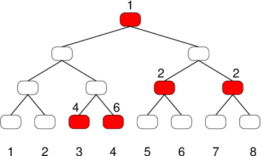
Figure 3: A q-digest formed over the value range [1,8]. The complete tree of buckets is shown and the buckets that actually exist on the q-digest are highlighted in red. The numbers next to the filled buckets show how many values were counted within that bucket. For this q-digest, $n=15,U=8$ and the threshold $\lfloor n\rho/\log U\rfloor=3$ (see eqns. 3, 4).

Intuitively a q-digest has many similarities to a equi-depth histogram: the buckets correspond to the histogram buckets and we strive to maintain the q-digest such that all buckets have roughly equal counts. The memory footprint of the q-digest is proportional to the number of buckets. Therefore to reduce memory consumption, we can take two sibling buckets and merge them with the parent bucket. The merge is done by deleting both the children and then adding their counts to the parent bucket. The merge step loses information, since the counts of both the children are lost, but reduces memory consumption.

Formally speaking, a q-digest with error parameter $\rho$, is a subset of all possible buckets such that it satisfies the following q-digest invariant. Suppose that the total number of values counted within the q-digest is $n$. Then any bucket $b$ in the q-digest satisfies the following two properties:

$$\rm{count}(b) \leq \left\lfloor\frac{n\rho}{\log U}\right\rfloor$$ (3)

$$\rm{count}(b)+\rm{count}(b_{p})+\rm{count}(b_{s}) > \left\lfloor\frac{n\rho}{\log U}\right\rfloor$$ (4)

where $b_{p}$ is the parent bucket of $b$ and $b_{s}$ is the sibling bucket of $b$. The first property (3) ensures that none of the buckets are too heavy and hence attempts to preserve accuracy being lost by merging too many buckets. The only exception to this property is the leaf bucket, which due to integer value assumption cannot be divided any further. The second property (4) ensures that the total values counted in a bucket, its sibling and parent are not too few; therefore it encourages merging of buckets to reduce memory. The only exception to this property is the root bucket since it does not have a parent.

The q-digest supports two basic operations: Insert and Compress. Below, we show how we extend this q-digest structure to implement our VariableBucket algorithm and how the basic operations work.

3.2.2 Variable Buckets Using q-digest

foreach item $v_{ij}$ in the braid do if bucket $b=[v_{ij},v_{ij}]$ does not exist then create bucket $b$ ;

end insert $i$ into CMSketch($b$);

increment count($b$) ;

if $b$ and its parent and sibling violates q-digest property then Compress end end

Algorithm 2 VariableBucket Insert Algorithm

for $\ell=0$ to $(\log U-1)$ do foreach bucket $b$ in level $\ell$ do if $\textrm{count}(b)+\textrm{count}(b_{p})+\textrm{count}(b_{s})<\lfloor n\rho/\log U\rfloor$ then count($b_{p}$) $\leftarrow$ count($b$) + count ($b_{s}$) ;

CMSketch($b_{p}$) $\leftarrow$ CMSketch($b_{p}$) $\cup$ CMSketch($b$) $\cup$ CMSketch($b_{s}$) ;

delete $b$ and $b_{s}$ ;

end end end

Algorithm 3 VariableBucket Compress Algorithm

The VariableBucket algorithm can be understood as a derivative of the q-digest data structure. In the basic q-digest, we divide the input values into $\rho^{-1}\log U$ buckets and in each bucket we count the values in that bucket using a simple counter. In the VariableBucket synopsis, we augment this simple counter by an CM sketch of size $O(\varepsilon^{-1}\log\delta^{-1})$.

Initially the q-digest starts out empty with no buckets. When processing the next value $v_{ij}$ (the $j$-th value in stream $i$) in the stream, we first check the q-digest to see if the leaf bucket $[v_{ij},v_{ij}]$ exists. If it exists, then we insert the stream id $i$ into the CM sketch for that bucket and increment the counter for that bucket by 1. If that bucket does not exist, then we create a new $[v_{ij},v_{ij}]$ bucket and insert the pair into that bucket. After adding the pair, we carry out a Compress operation on the q-digest. As more and more data is inserted into the VariableBucket structure, the buckets are automatically merged and reorganized by the Compress operation. This adaptive bucket structure is the reason for the name VariableBucket.

Given this data structure, let us now see how to approximate the median value of a stream $i$. First we estimate $n_{i}$ by taking the union of all the CM sketches in each bucket and then querying it for the value of $n_{i}$. We then do a post-order traversal of the q-digest tree and merge the CM sketches of all the buckets visited. As we merge the CM sketches, we check the value of the count for stream $i$. Suppose when we merge bucket $b$ to the unified CM sketch, the number of values in the unified CM sketch exceeds $n_{i}/2$. Then we report the right edge of the bucket $b$ as our estimate for the median.

This estimate has three sources of error. The first error is in the estimate of $n_{i}$ itself, which is at most $\varepsilon n$ using the CM sketch error bound. The second source of error is from estimating the value of $n_{i}/2$ while taking union of multiple CM sketches and this error is again $\varepsilon n$. The third error is from the error in count of $i$ in bucket $b$. This error arises from the fact that any value which is counted in bucket $b$ can be counted on its ancestors as well, because the bucket $b$ overlaps with all its ancestors. Since there are at most $\log U$ ancestors and every ancestor has count at most $n\rho/\log U$ (eqn. 3), the total error is $n\rho$ from this source. Therefore the total error is $2\varepsilon n+\rho n$. By rescaling $\varepsilon$ by a factor of two, and setting $\rho=\varepsilon$, we arrive at the following theorem.

Theorem 3.9.

The VariableBucket is a data structure of size $O(\varepsilon^{-2}\log U\log\delta^{-1})$ that, with probability at least $1-\delta$, can find the top $k$ streams in a set of $m$ streams by average, median, or any quantile value, with (additive) rank approximation error $\varepsilon n$, where $n$ is the total size of all the streams in the braid.

Similarly, we can find top $k$ streams using other measures such as 95th percentile, average, etc.

4 Experimental Results

In this section, we discuss our empirical results. We implemented both of our schemes ExponentialBucket and VariableBucket and evaluated them on a variety of datasets. In all of our experiments we found that VariableBucket consistently outperformed ExponentialBucket and the main advantage of ExponentialBucket is its somewhat smaller memory usage. (However, the memory advantage is at most a factor of 2.) Therefore, we report all performance numbers for the VariableBucket only and later show one experiment comparing the relative performance of the two schemes.

We focused on three most common statistical measures of streams: the median, the 95th percentile, and the average value. Our goal in these experiments was to evaluate the effectiveness of these schemes in extracting the top $k$ streams using these measures. We used the following performance metrics for this evaluation.

1. Precision and Recall: Precision is the most basic measure for quantifying the success rate of an information retrieval system. If $\mathcal{S}(k)$ is the true set of top $k$ streams under a weight function and $\mathcal{S}^{\prime}(k)$ is the set of streams returned by our algorithms, then the precision at $k$ $P(k)$ of our scheme is defined as

   $$P(k)\>=\>\frac{|\mathcal{S}(k)\cap\mathcal{S}^{\prime}(k)|}{|\mathcal{S}(k)|}=\frac{|\mathcal{S}(k)\cap\mathcal{S}^{\prime}(k)|}{k}.$$ (5)

   Thus, precision provides the relative measure of how many of the top $k$ are found by our scheme. The precision values always lie between $0$ and $1$, and closer the precision to $1.0$, the better the algorithm. We note that in this particular case, precision is the same as recall, defined as

   $$R(k)\>=\>\frac{|\mathcal{S}(k)\cap\mathcal{S}^{\prime}(k)|}{|\mathcal{S}^{\prime}(k)|}=\frac{|\mathcal{S}(k)\cap\mathcal{S}^{\prime}(k)|}{k}.$$ (6)

   since $|\mathcal{S}(k)|=|\mathcal{S}^{\prime}(k)|$.

2. Distortion: The precision is a good measure of the fraction of top $k$ streams found by our algorithm, but it fails to capture the ranking of those streams. For example, suppose we have two algorithms, and both correctly return the top 10 streams but one returns them in the correct rank order while the other returns them in the reverse order. Both algorithms enjoy a precision of 1.0 but clearly the second one performs poorly in its ranking of the streams. Our distortion measure is meant to capture this ranking quality. Suppose for a stream $S_{i}$ the true rank is $r(S_{i})$, while our heuristic ranks it as $r^{\prime}(S_{i})$. Then, we define the (rank) distortion for stream $S_{i}$ to be

   $$d_{i}\>=\>\left\{\begin{array}[]{l}r(S_{i})/r^{\prime}(S_{i}),\quad\mbox{if}~{}r(S_{i})\geq r^{\prime}(S_{i})\\ r^{\prime}(S_{i})/r(S_{i}),\quad\mbox{otherwise}.\end{array}\right.$$

   The overall distortion is taken to be the average distortion for the $k$ streams identified by our scheme as top $k$. The ideal distortion is 1, while the worst distortion can be $\Theta(m/k)$, where $m$ is the size of the braid: this happens when the algorithm ranks the bottom $k$ streams as top $k$, for $k\ll m$. Thus, smaller the distortion, the better the algorithm.

3. Value Error: Both precision and distortion are purely rank-based measures, and ignore the actual values of the weight function $\lambda(S)$. In the cases when data is clustered, many streams can have roughly the same $\lambda$ value, yet be far apart in their absolute ranks. Since in many monitoring application, we care about streams with large weights, a user may be perfectly satisfied with any stream whose weight is close to the weights of true top $k$ streams. With this motivation, we define a value-based error metric, as follows. Suppose the true and approximate streams at rank $k$ are $S_{k}$ and $S_{k}^{\prime}$. Then the relative value error $e(k)$ is defined as

   $$e(k)=\left|\frac{\lambda(S_{k})-\lambda(S_{k}^{\prime})}{\lambda(S_{k})}\right|$$ (7)

   The average value error $e$ for the top $k$ is then defined as the average of $e(k)$ over all $k$ streams.

4. Memory Consumption: The space bounds that our theorems give are unduly pessimistic. Therefore we also empirically evaluated the memory usage of our scheme.

We generate several synthetic data sets using natural distributions to evaluate the performance and quality of our algorithms. In all cases, we use 1000 streams, with about 5000 items each, for the total size of all the streams 5M. In all cases, the values within each stream are distributed using a Normal distribution with variance $U/20$. The mean values for each distribution are picked by an inter-stream distribution, for which we try 3 different distributions: uniform, outlier, and normal.

• In the Uniform distribution, we pick values uniformly at random from the range $U=[1,2^{16}]$, and each such value acts as the mean $\mu_{i}$ for stream $S_{i}$.

• In the Outlier distributions, we choose 900 of the streams with values in the range $[0,0.6U]$ and the remaining 100 streams in the range $[aU,(a+0.2)U]$, with $a<1$, for different values of $a$.

• In the Normal distribution, the values are chosen from a normal distribution with mean $2^{15}$, and standard deviation $2^{14}$.

4.1 Precision

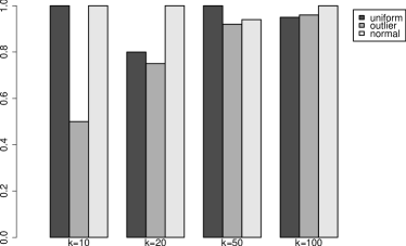
(a) Precision for $\lambda$=average

(b) Precision for $\lambda$=median

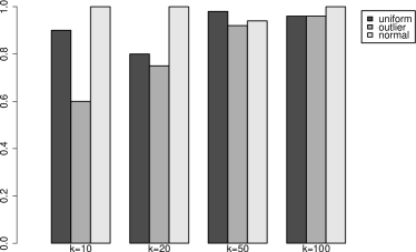
(c) Precision for $\lambda$=95th percentile

Figure 4: The precision quality of VariableBucket as a function of $k$, for the three choices of $\lambda$: average, median, and 95th percentile.

Our first experiment evaluates the precision quality: how many of the true top $k$ streams are correctly identified by our algorithms. Figure 4 shows the results of this experiment, where for each data set (of 1000 streams), we asked for the top $k$, for $k=10,20,50,100$. In Figure 4 the outlier distribution has parameter $a=0.8$. We evaluated the precision for each of the three choices of $\lambda$: average, median, and 95th percentile. As the figure shows, the precision quality of VariableBucket begins to approach 100% for $k\geq 50$. The pattern is similar for average, median, or the 95th percentile. The precision achieved by VariableBucket on the outlier distribution degrades as the parameter $a$ decreases. as it can be seen in Figure 5. This behavior is easily explained by the fact that the parameter $\alpha$ sets the separation between outlier and non-outlier streams. The smaller $\alpha$ is, the fuzzier becomes the separation, therefore VariableBucket success rate in identifying outliers decreases.

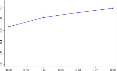
Figure 5: Precision achieved by VariableBucket for different $a$ in the outlier distribution, top-100, $\lambda$=median

4.2 Distortion Performance

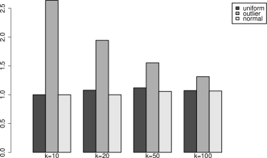
(a) Distortion for $\lambda$=average

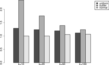
(b) Distortion for $\lambda$=median

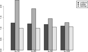
(c) Distortion for $\lambda$=95th percentile

Figure 6: The distortion performance of VariableBucket as a function of $k$, for the three choices of $\lambda$: average, median, and 95th percentile.

Our second experiment measures distortion in ranking the top $k$ streams, under the three weight functions average, median, and 95th percentile. The results are shown in Figure 6. For all three data sets, distortion is uniformly small (between 1 and 4), even for $k$ as small as 10, and it actually drops to the range 1–2 for $k\geq 50$.

4.3 Average Value Error

(a) Average value error for $\lambda$=average

(b) Average value error for $\lambda$=median

Figure 7: The average value error of VariableBucket as a function of $k$, for the three choices of $\lambda$: average, median, and 95th percentile.

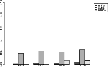
(c) Precision for median $\lambda$=95th percentile

The previous two experiments have attempted to measure the quality of our scheme using a rank-based metric. In this section, we consider the performance using the value error, as defined earlier. The results are shown in Figure 4.3. For all distributions, the relative error in the value of the top $k$ streams is quite small: of the order of 1–2%. Thus, even when the algorithm finds streams outside the true top $k$, it is identifying streams that are close in value to the true top $k$. This is especially encouraging because in data without clear outliers, the meaning of top $k$ is always a bit fuzzy.

4.4 ExponentialBucket vs. VariableBucket

In our experiments, we tried both our schemes, ExponentialBucket and VariableBucket, on all the data sets, but due to the space limitation, we reported all the results using VariableBucket only. In this section, we show one comparison of the two schemes to highlight their relative performance. Figure 8 shows the results for the precision using the median weight, for all three data sets. The bottom figure is the same one as in Figure 4 (middle), while the top one shows the performance of ExponentialBucket for this experiment. One can see that in general VariableBucket delivers better precision than ExponentialBucket. This was our observation in nearly all the experiments, leading us to conclude that VariableBucket has better precision and error guarantees than ExponentialBucket. This is also consistent with out theory, where we found that VariableBucket can be shown to have bounded rank error guarantee while ExponentialBucket could not. On the other hand, ExponentialBucket does have a memory advantage: its data structure consistently was more space-efficient that that of VariableBucket, so when space is a major constraint, ExponentialBucket may be preferable. However, the space usage of VariableBucket itself is not prohibitive, as we show in the following experiment.

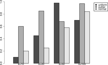
(a) Precision for median, ExponentialBucket

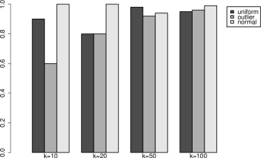
(b) Precision for median, VariableBucket

Figure 8: A comparison of ExponentialBucket with VariableBucket. The ExponentialBucket is more space-efficient but consistently does worse than VariableBucket. This experiment shows, side-by-side, the results of the precision quality experiment for the median weight, using the two schemes.

4.5 Memory Usage

In this experiment, we evaluated how the memory usage of VariableBucket scales with the size of the braid. In theory, the size of VariableBucket does not grow with $m$, the number of streams, or the size of individual streams. However, theoretical bounds on the space size are highly pessimistic, so used this experiment to evaluate the space usage in practice. In our implementation of VariableBucket we used a Count-Min sketch with depth 64 and width 64. We then built VariableBucket for number of streams varying from $m=1000$ to $m=10,000$, and Figure 9 plots the memory usage vs. the number of streams. As predicted, the data structure size remains virtually constant, and is about 2 MB.

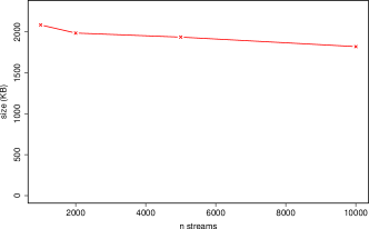
Figure 9: Data structure size as a function of the braid size.

5 Conclusion

We investigated the problem of tracking outlier streams in a large set (braid) of streams in the one-pass streaming model of computation, using a variety of natural measures such as average, median, or quantiles. These problems are motivated by monitoring of performance in large, shared systems. We show that beyond the simplest of the measures (max or min), these problems immediately become provably hard and require space linear in the braid size to even approximate. It seems surprising that the problem remains hard even for such minor extensions of the max as the “second maximum” or the spread ($\max-\min$), or that even highly structured streams with the round robin order remain inapproximable. We also propose two heuristics, ExponentialBucket and VariableBucket, analyzed their performance guarantees and evaluated their empirical performance.

There are several directions for future work. For instance, we observed that the different Count-Min sketches are used quite unevenly. Some sketches are populated to the point of saturation, making their error estimates quite bad while others are hardly used. This suggest that one could improve the performance of our data structures by an adaptive allocation of memory to the different sketches so that heavily trafficked sketches receive more memory than others.

References

- [1] N. Alon, Y. Matias, and M. Szegedy. The space complexity of approximating the frequency moments. In Proc. of STOC, 1996.
- [2] Z. Bar-Yossef, T. S. Jayram, R. Kumar, and D. Sivakumar. An information statistics approach to data stream and communication complexity. J. Comput. Syst. Sci., 68(4):702–732, 2004.
- [3] F. Bonomi, M. Mitzenmacher, R. Panigrahi, S. Singh, and G. Varghese. Beyond bloom filters: from approximate membership checks to approximate state machines. Proc. Sigcomm, 36(4):315–326, 2006.
- [4] M. Charikar and K. Chen M. Farach-Colton. Finding frequent items in data streams. Theoretical Computer Science, 312(1):3–15, 2004.
- [5] G. Cormode and M. M. Hadjieleftheriou. Finding frequent items in data streams. Proceedings of VLDB, 1(2):1530–1541, 2008.
- [6] G. Cormode and S. Muthukrishnan. An improved data stream summary: the count-min sketch and its applications. Journal of Algorithms, 55(1):58–75, 2005.
- [7] Christos Faloutsos, M. Ranganathan, and Yannis Manolopoulos. Fast subsequence matching in time-series databases. In SIGMOD Conference, 1994.
- [8] L. Fan, P. Cao, J. Almeida, and A. Z. Broder. Summary cache: A scalable wide-area web cache sharing protocol. In IEEE/ACM Transactions on Networking, pages 254–265, 1998.
- [9] M. Greenwald and S. Khanna. Space-efficient online computation of quantile summaries. In Proc. of ACM SIGMOD, pages 58–66, 2001.
- [10] R. M. Karp, S. Shenker, and C. H. Papadimitriou. A simple algorithm for finding frequent elements in streams and bags. ACM TODS, 28(1):51–55, 2003.
- [11] Eamonn J. Keogh, Jessica Lin, and Ada Wai-Chee Fu. Hot sax: Efficiently finding the most unusual time series subsequence. In ICDM, 2005.
- [12] G. S. Manku and R. Motwani. Approximate frequency counts over data streams. In Proceedings of VLDB, pages 346–357, 2002.
- [13] A. Metwally, D. Agrawal, and A. El Abbadi. Efficient computation of frequent and top-k elements in data streams. In Proceedings of ICDT, pages 398–412, 2005.
- [14] J. Misra and D. Gries. Finding repeated elements. Sci. Comput. Programming, pages 143–152, 1982.
- [15] I. Munro and M. S. Paterson. Selection and sorting with limited storage. Theoretical Computer Science, pages 315–323, 1980.
- [16] Noam Nisan and Eyal Kushilevitz. Cambridge University Press, 1997.
- [17] R. Schweller, Z. Li, Y. Chen, Y. Gao, A. Gupta, Y. Zhang, P. Dinda, M. Kao, and G. Memik. Reversible sketches: enabling monitoring and analysis over high-speed data streams. IEEE/ACM Transactions on Networking, 15:1059–1072, 2007.
- [18] N. Shrivastava, C. Buragohain, D. Agrawal, and S. Suri. Medians and beyond: new aggregation techniques for sensor networks. In Proc. of ACM SenSys, pages 239–249, 2004.
- [19] Andrew Chi-Chih Yao. Some complexity questions related to distributive computing(preliminary report). In ACM STOC, 1979.