Numerical simulations of the energy- supercritical Nonlinear Schrödinger equation

Abstract.

We present numerical simulations of the defocusing nonlinear Schrödinger (NLS) equation with an energy supercritical nonlinearity. These computations were motivated by recent works of Kenig-Merle and Kilip-Visan who considered some energy supercritical wave equations and proved that if the solution is a priori bounded in the critical Sobolev space (i.e. the space whose homogeneous norm is invariant under the scaling leaving the equation invariant), then it exists for all time and scatters.

In this paper, we numerically investigate the boundedness of the $H^{2}$-critical Sobolev norm for solutions of the NLS equation in dimension five with quintic nonlinearity. We find that for a class of initial conditions, this norm remains bounded, the solution exists for long time, and scatters.

1. Introduction

This paper is a numerical investigation of wellposedness and scattering properties of solutions of the defocusing nonlinear Schrödinger (NLS) equation,

(1.1) $$\mathrm{i}u_{t}+\Delta u-\lvert u\rvert^{p-1}u=0,\quad u:\mathbb{R}^{d}\times\mathbb{R}\to\mathbb{C}$$

in the energy supercritical setting. The notion of $H^{s}$-criticality is associated with the scaling transformation $u(x,t)\to u_{\lambda}(x,t)=\lambda^{2/(p-1)}u(\lambda x,\lambda^{2}t)$ that leaves the NLS equation invariant. We say that the problem is $H^{s}$-critical, if the homogeneous $H^{s}$-norm of the solution remains unchanged under the above scaling. We place ourselves in the energy ($H^{1}$) supercritical regime by assuming that the dimension and the nonlinearity are such that the critical Sobolev exponent $s_{c}$ satisfies

(1.2) $$s_{c}\equiv\frac{d}{2}-\frac{2}{p-1}>1.$$

The two conserved quantities of the NLS equation, the mass

(1.3) $$M(u)=\int_{\mathbb{R}^{d}}|u(x,t)|^{2}dx$$

and the energy

(1.4) $$E(u)=\int_{\mathbb{R}^{d}}(|\nabla u(x,t)|^{2}+\frac{1}{p+1}|u|^{p+1})dx$$

have indeed led to a special interest to mass-critical ($s_{c}=0$) and energy-critical ($s_{c}=1$) problems.

Significant progress on global well-posedness and scattering has been made since the pioneering work on scattering by Ginibre and Velo [8], Lin and Strauss [18], and Strauss [22]. In these early works, scattering was shown to hold for a range of energy subcritical configurations with finite variance. Subsequent work [9] proved scattering in the energy space. These results, and refinements, are collected in [23], [25], [4].

For energy subcritical problems with $s_{c}<1$, global well-posedness and scattering results have been obtained for $H^{s}$ data with $s$ near 1 and away from $s_{c}$. Bourgain [1] established scattering in $H^{s}$, for radially symmetric data, for all $s\in(11/3,1)$. This was refined by Colliander, Keel, Staffilani, Tao and Takaoka [5], where the solution emerging from general initial data was shown to scatter for $s\in(4/5,1)$. These results establish global well-posedness and scattering for some data which have infinite energy.

Scattering results at critical regularity have been established starting ten years ago. A breakthrough result [2] on the 3d energy critical problem for radial data established a new strategy for proving scattering for initial data of critical regularity. With other ideas in [6], Bourgain’s induction-on-energy strategy resolved the case for general data. The 4 dimensional defocusing energy critical case was then established by Ryckman and Visan [20] with the higher dimensional case thereafter [27]. Other important advances on the energy critical problem appear in [10], [26]. Scattering was obtained [11] beneath the natural threshold size for the focusing energy critical problem. Moreover, ideas in [11, 13] simplified the implementation of the energy critical strategy leading to advances on other model equations. Building on these developments, scattering in the $L^{2}$-critical problem for large radial $L^{2}$ data was established in the defocusing case [15] and for radial data under the ground state mass in the focusing case [17] .

Scattering is expected to hold for general large data of critical regularity for (1.1). To date, no such result has been established except in the energy critical case. Under the assumption of bounded critical norm, the defocusing $H^{1/2}$ case has been shown [12] to scatter for large critical data.

The hypothesis of a bounded critical Sobolev norm has recently been considered in the energy supercritical regime $s_{c}>1.$ Following a recent work by Kenig and Merle [14] on the energy supercritical wave equation, Killip and Visan [16] considered some classes of energy supercritical NLS equations in dimension $d\geq 5$ and proved that if the solution is a priori bounded in the critical Sobolev space $H^{s_{c}}$, it exits for all time and scatters.

The purpose of our study is to investigate numerically the latter assumption on the critical Sobolev norm. We are also motivated by the discussion of the “theoretical possibility for computer assisted proofs of global well-posedness and scattering” appearing in [3]. We have performed our computations in the case $d=5$ with quintic nonlinearity ($p=5$). This is the ‘simplest’ case when the critical exponent is the smallest possible integer; $s_{c}=2$. In addition, we assume the initial conditions are spherically symmetric to simplify the computations. Note that our choice of dimension and nonlinearity is not exactly covered by Theorems 1.4 and 1.5 of [16], although the authors claim that their result can be extended to any power law nonlinearity $|u|^{p-1}u$ with $p$ odd integer, and $s_{c}<p$.

The main observation of our numerical work is that, for the various initial conditions we have considered, the critical norm $\dot{H}^{2}$ of the solution remains bounded for all time and that the solution scatters. As time evolves and the solution reaches an asymptotic state, the energy concentrates into the kinetic energy and the potential energy tends to zero. At the same time, the $\dot{H}^{2}$ norm of the solution stabilizes to some value. This value may be much higher than that of the initial conditions. For a more quantitative assessment of the solution in the frequency space, we also calculate the norm of the solution in the Besov space $\dot{B}^{2}_{2,\infty}$. Let $P_{j}$ be the Fourier multiplier operator which projects the Fourier transform of a function $f$ onto the annulus $2^{j}\leq|\xi|<2^{j+1}$. The Besov $\dot{B}^{s}_{2,\infty}(\mathbb{R}^{d})$ is equipped with the norm

(1.5) $$\sup_{j\in\mathbb{Z}}2^{2j}\|P_{j}f\|_{L^{2}_{x}}.$$

We observe that the $H^{2}$ density spreads out in Fourier space and the $B^{2}_{2,\infty}$ norm shrinks to small values as time advances under (1.1). The emergent small Besov norm and Strichartz refinements (such as those appearing in the work [19] of Planchon and references therein) gives further evidence of scattering for solutions of (1.1) and provides a smallness mechanism for possibly implementing the computer assisted proof described in [3].

In Section 2 we describe our numerical schemes and in Section 3 we present our main results.

2. Numerical Methods

2.1. Time and Space Discretization

We study (1.1) with $d=5$ and $p=5$ and radially symmetric data. This configuration is convenient because the $\dot{H}^{2}$ norm is bounded by the $L^{2}$ norm of $\Delta u$.

To simulate the problem, we first truncate the domain, restricting $r\in(0,R_{\max})$, with boundary conditions

(2.1) $$u_{r}\mid_{r=0}=0,\qquad u(r=R_{\max})=0.$$

These are interpreted as a symmetry condition at the origin, and an infinite barrier at $r=R_{\max}$ so that $u=0$ at all $r>R_{\max}$. $R_{\max}$ must be sufficiently large to avoid boundary interaction. The domain is discretized as

(2.2) $$0=r_{0}<r_{1}<r_{2}<\ldots<r_{j}=jh<\ldots<r_{N}=L.$$

Letting $U_{j}(t)=u(r_{j},t)$, the fourth order spatial discretization is

(2.3) $$\begin{split}&\imath\dot{U}_{j}+\frac{-U_{j-2}+16U_{j-1}-30U_{j}+16U_{j+1}-U_{j+2}}{12h^{2}}\\ &\quad+\frac{4}{r_{j}}\frac{U_{j-2}-8U_{j-1}+8U_{j+1}-U_{j+2}}{12h}=\lvert U_{j}\rvert^{4}U_{j}.\end{split}$$

and the discretized boundary conditions are:

(2.4) $$U_{-1}=U_{1}\;;\;U_{-2}=U_{2},$$

(2.5) $$U_{N+1}=0\;;\;U_{N+2}=0.$$

We integrate in time using the classical fourth order Runge-Kutta scheme with $\Delta t=O(\Delta r^{2})$ to ensure numerical stability.

2.2. Fourier Transform

We need to compute the Fourier transform of the solution to evaluate its norm in the Besov space. The Fourier transform of a radial function in $\mathbb{R}^{d}$ at $k=\lvert\mathbf{k}\rvert$ is

(2.6) $$\hat{u}(k)=\frac{1}{k^{\nu}}\int_{0}^{\infty}u(r)J_{\nu}(kr)r^{d/2}dr,\quad\nu=\frac{d-2}{2}.$$

This formula is derived in many texts on the Fourier transform, including Stein and Weiss [21]. Indeed, for radially symetric functions,

$$\hat{u}(\mathbf{k})=\frac{1}{(2\pi)^{d/2}}\int_{\mathbb{R}^{d}}e^{-i\mathbf{k}\cdot\mathbf{x}}u(\mathbf{x})d\mathbf{x}=\frac{1}{(2\pi)^{d/2}}\int_{0}^{\infty}\left\{\int_{\partial B_{0}(1)}e^{-ikr\hat{\mathbf{k}}\cdot\mathbf{y}}dS_{\mathbf{y}}\right\}u(r)r^{d-1}dr.$$

The kernel is

$$\int_{\partial B_{0}(1)}e^{-ikr\hat{\mathbf{k}}\cdot\mathbf{y}}dS_{\mathbf{y}}=(2\pi)^{d/2}(kr)^{-(d-2)/2}J_{(d-2)/2}(kr),$$

leading to expression 2.6.

Following Cree and Bones [7], we approximate the integral as follows. For $k>0$, we use the trapezoidal rule at the grid points $r_{j}=j\Delta r$, $\Delta r=R_{\max}/N$ and $j=0,1,\ldots,N$. At $k=0$, we instead approximate the integral

(2.7) $$\hat{u}(k=0)=\frac{1}{2^{\nu}\Gamma(1+\nu)}\int_{0}^{\infty}u(r)r^{\nu+d/2}dr.$$

The Nyquist frequency, $K_{\max}$, is related to our discretization by the expression:

$$K_{\max}R_{\max}=\frac{N}{2}.$$

The Fourier transform is computed at the points $k_{j}=j\Delta k$, $\Delta k=1/(2R_{\max})$ and $j=0,1,\ldots,N$. As discussed in their article, Cree and Bones found this method to be robust, though it is slow.

2.3. Besov Approximation

We now approximate the Besov space norm

(2.8) $$\lVert u\rVert_{\dot{B}^{2}_{2,\infty}}=\sup_{j\in\mathbb{Z}}2^{2j}\lVert\hat{u}\rVert_{L^{2}([2^{j},2^{j+1}))}$$

For this purpose, we first identify values of $j$ for which these integrals can be meaningfully computed by the trapezoidal rule. Let

(2.9) $$j_{\min} =\mathrm{ceil}(\log(4k_{1})/\log(2))$$

(2.10) $$j_{\max} =\mathrm{floor}(\log(k_{N})/\log(2))$$

We choose $j_{\min}$ to guarantee at least four grid points $<2^{j_{\min}}$. For $j_{\min}\leq j\leq j_{\max}-1$, the integral

(2.11) $$\lVert\hat{u}\rVert_{L^{2}([2^{j},2^{j+1}))}^{2}=\int_{2^{j}}^{2^{j+1}}\lvert\hat{u}\rvert^{2}dk\approx q_{j}^{2}$$

is computed by the trapezoidal rule. We also compute

(2.12) $$\lVert\hat{u}\rVert_{L^{2}([0,2^{j_{\min}}))}^{2}=\int_{0}^{2^{j_{\min}}}\lvert\hat{u}\rvert^{2}dk\approx q_{j_{\min}-1}^{2}$$

and

(2.13) $$\lVert\hat{u}\rVert_{L^{2}([2^{j_{\max}},K_{\max}])}^{2}=\int_{2^{j}_{\max}}^{K_{\max}}\lvert\hat{u}\rvert^{2}dk\approx q_{j_{\max}}^{2}$$

With these integrals in hand,

(2.14) $$\lVert u\rVert_{\dot{B}^{2}_{2,\infty}}\approx\max_{j_{\min}-1\leq j\leq j_{\max}}\left\{2^{2j}q_{j}\right\}$$

2.4. Error of Numerical Scheme

We have tested our scheme by varying both the domain size and the grid resolution. In Table 1, we show two metrics of our simulations, the value of $\lvert u\rvert$ at the origin, and the maximum of $\lvert u\rvert$ at a fixed time. We see consistency amongst the simulations for the different parameters. Examining the tails of $\lvert u\rvert$ in Figure 1, we get a qualitative assessment of how these parameters influence the simulation. So long as we have not reached the edge of the domain, which none of these simulations have, $R_{\max}$ matters little. In the better resolved simulations, $\lvert u\rvert$ has propogated farther too the right. This is expected since greater resolution resolves higher wave numbers. As will be argued in the next section, $u$ is scattering, and thus obeys the linear equation, where higher frequencies propagate with greater speed.

No. Points	$R_{\max}$	$\lvert u\rvert(r=0)$	$\max_{r\in[0,R_{\max}]}\lvert u\rvert$
10000	100	0.7126025579	2.665689301
20000	100	0.712561663	2.665668567
40000	100	0.7125588732	2.665667313
20000	200	0.7126025586	2.665689301
40000	200	0.7125616583	2.665668567
200000	2000	0.7126025579	2.665689301

Table 1. Convergence of $\lvert u\rvert(r=0)$ and $\max_{r}\lvert u\rvert$ for Gaussian data $u_{0}=10e^{-r^{2}}$ at $t=.02$.

The discretization scheme is neither mass nor energy conservative. A calculation of the relative error on these conserved quantities is another measure of accuracy. Table 2 shows that the spatial resolution for our various initial conditions and the relative error for the two invariants. As expected, the simulations with better spatial resolution, hence better temporal resolution, better conserve the invariants. These invariants were computed by Simpson’s method on the interval $[0,R_{\max}]$ with the discrete densities

$$\left[(\Re U_{i})^{2}+(\Im U_{i})^{2}\right]r_{i}^{4}$$

and

$$\left[-(\Re U_{i}\Delta_{\textrm{disc.}}\Re U_{i})-(\Im U_{i}\Delta_{\textrm{disc.}}\Im U_{i})+\frac{2}{p+1}\left((\Re U_{i})^{2}+(\Im U_{i})^{2}\right)^{6}\right]r_{i}^{4}.$$

$\Delta_{\textrm{disc.}}$ is the discrete Laplacian from (2.3).

Initial Condition	No. Points	$R_{\max}$	$T_{\max}$	$\max_{t}\lvert\%\Delta\mathrm{Mass}\rvert$	$\max_{t}\lvert\%\Delta\mathrm{Energy}\rvert$
Gaussian, $u_{0}=10e^{-r^{2}}$	40001	100	0.04	6.55478e-09	2.67077e-08
Gaussian, $u_{0}=10e^{-r^{2}}$	200001	2000	3.2	1.97657e-06	7.94582e-06
Ring, $u_{0}=8r^{2}e^{-r^{2}}$	32001	100	0.2	2.33731e-10	2.19067e-09
Ring, $u_{0}=8r^{2}e^{-r^{2}}$	120001	2400	9.0	9.61835e-07	8.70909e-05
Osc. Gaussian, $u_{0}=4e^{-10\mathrm{i}r^{2}}e^{-r^{2}}$	40001	100	0.1	1.35194e-08	1.8279e-08
Osc. Gaussian, $u_{0}=4e^{-10\mathrm{i}r^{2}}e^{-r^{2}}$	200001	1000	1.0	2.15647e-07	2.91404e-07

Table 2. Error in the conserved quantities for each simulation.

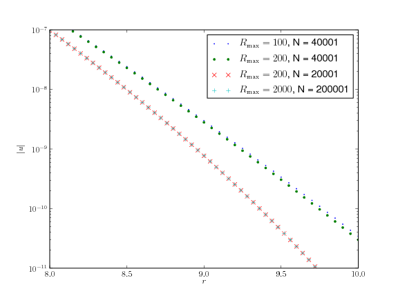
Figure 1. Variation in the tails of $\lvert u\rvert$ at $t=.04$ for Gaussian data $u_{0}=10e^{-r^{2}}$.

We also verify our time stepping and Fourier approximation by simulating a linear problem, computing the approximate Fourier transform, and observing that it does not change in time; see Figure 2.

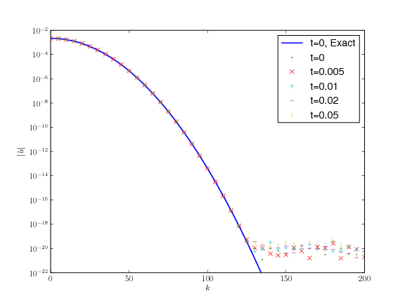
Figure 2. Fourier transform at various times of a linear Schrödinger equation simulation with initial condition $u_{0}=4e^{-10\mathrm{i}r^{2}}e^{-r^{2}}$

3. Numerical Observations

In this section we present and discuss our numerical simulations for energy supercritical defocusing NLS, (1.1). Throughout, our initial conditions are radially symmetric, simplifying the computations. We speculate that the dynamics persist for general data and for other energy supercritical configurations.

3.1. Initial Conditions

We consider several families of initial conditions. These are:

Gaussians:

(3.1) $$u_{0}(r)=Ae^{-r^{2}}$$

Under the linear flow, these are well known to spread and decay in $L^{\infty}$. Our simulations show the nonlinear distortion in the shape.

Rings:

(3.2) $$u_{0}(r)=Ar^{2}e^{-r^{2}}$$

Oscillatory Gaussians:

(3.3) $$u_{0}(r)=Ae^{-\alpha\mathrm{i}r^{2}}e^{-r^{2}}$$

Under the linear flow with $\alpha>0$, such an initial condition will initially focus towards the origin, then relax and decay. Our simulations show that the nonlinearity arrests this focusing.

In all cases, the amplitude $A$ is taken “large enough” so that the nonlinear effects in (1.1) will, at least initially, be strong and we will be outside the small data regime where scattering is known to occur [25]. We present the following cases: Gaussian data with $A=10$, $u_{0}=10e^{-r^{2}}$; Ring data with $A=8$, $u_{0}=8r^{2}e^{-r^{2}}$; Oscillating Gaussian data with $A=4$ and $\alpha=10$, $u_{0}=4e^{-10\mathrm{i}r^{2}}e^{-r^{2}}$.

3.2. Results

In all simulations, we find that after a transient period, the solution remains smooth and monotonically decays in amplitude. This is evidence of global well-posedness. The $L^{\infty}$ smallness of the solution is a first indication of scattering, as the nonlinearity becomes a perturbation of the linear equation. After this transient period, the $L^{6}$-norm also decays monotonically. Since the energy invariant is conserved, the potential energy is absorbed by the kinetic term, as is expected in scattering. We also study the evolution of the $L^{14}_{x}$-norm, which is important because, by Strichartz,

$$\lVert e^{i\Delta t}u_{0}\rVert_{L^{14}_{t,x}}\leq C\lVert u_{0}\rVert_{\dot{H}^{2}}.$$

If the flow is to become asymptotically linear, we would expect $L^{14}_{x}$ to decay $\propto t^{-15/7}$, the theoretical rate of the linear flow. Indeed, when the simulation is run for a sufficiently long time, this is observed. Finally, there is the critical norm, $\dot{H}^{2}$. For numerical convenience we track $\lVert\Delta u\rVert_{L^{2}}$, which controls $\dot{H}^{2}$. Finally, our simulations indicate that $\lVert\Delta u\rVert_{L^{2}}$ saturates to a finite value. Thus, we have evidence that the scale invariant norm is globally bounded in time. This was the fundamental a assumption in [14, 16].

Let us examine the profiles from our simulations. The evolution of the Gaussian data, $u_{0}=10e^{-r^{2}}$ is plotted in Figure 3. The shape is distorted, but $\lvert u\rvert$ is monotonically decreasing in time. We can also see that oscillations in the shape spread. The ring data, $u_{0}=8r^{2}e^{-r^{2}}$, has more complex transient dynamics. As shown in Figure 4, there is initially a focusing of $u$ towards the origin. This subsequently relaxes, and $u$ spreads and decays in amplitude, much like the Gaussian data. The oscillatory gaussian, $u_{0}=4e^{-10\mathrm{i}r^{2}}e^{-r^{2}}$, is similar. It initially focuses, subsequently relaxes, and appears to scatter as in Figure 5.

For comparison, we simulate the linear Schrödinger equation with data $u_{0}=4e^{-10\mathrm{i}r^{2}}e^{-r^{2}}$ and the same discretization as in the nonlinear problem. Figure 6 shows much stronger focusing towards the origin than seen in Figure 5. The nonlinearity is arresting the rush towards the origin and keeps the amplitude orders of magnitude smaller.

For a more quantitative assessment of scattering, we examine the aforementioned integrated quantities. In Figure 7 (a) and (b), we plot $\lVert\Delta u\rVert_{L^{2}}$. Figure 7 (a) shows the rapid growth of this norm to $\sim 1200$, orders of magnitude larger than the initial value. Figure 7 (b), computed for a longer time, suggests that it has saturated at this value. As expected, the potential energy, $\int\lvert u\rvert^{6}$, vanishes. We see this in in Figures 7 (c) and (d), where we have plotted $\lVert u\rVert_{L^{6}}$ from the same two simulations. Lastly, in Figure 7 (f) the $L^{14}$ space norm, after a sufficient time, begins to decay as $\propto t^{-15/7}$.

The ring data and the oscillatory gaussian are, asymptotically, very similar. The same plots appear in Figures 8 and 9. We see rapid saturation of $\dot{H}^{2}$, the decay of the potential energy, and the asymptotically linear decay of the $L^{14}_{x}$ norm. One notable difference is that in the oscillating gaussian simulation, the initial focusing causes a decrease in $\dot{H}^{2}$ and an increase in the potential. Furthermore, the saturated value of $\lVert\Delta u\rVert_{L^{2}}$ is not appreciably larger than in its initial value. These simulations suggest there are at least two different time scales of interest. Saturation of $\dot{H}^{2}$ happen very rapidly. In contrast, the expected asymptotic decay of $L^{14}_{x}$ sets in at a much later time.

3.3. Fourier and Besov

Much of the recent analytical progress on NLS used careful treatment of the equation in the Fourier domain. We examine the Fourier transform of our simulations for hints that might be applied to future analysis. The transform, plotted at various times in Figures 7 (e), 8 (e), and 9 (e) shows several features. There is an initial spreading into high wave numbers, and the support is much broader than the initial condition. This relaxes, and the limiting state has a smaller support than during the transient period, but still in excess of the initial condition. The asymptotic constancy of the transform is further evidence that $u$ evolves linearly and scatters.

We can also interpret the Fourier data through the Besov norm (1.5). Using the method described in Section 2.3, we approximate the Besov norm $\dot{B}^{2}_{2,\infty}$ at several times in each simulation. This data, appearing as $\times$’s in Figures 7 (a), 8 (a), and 9 (a), shows several things. First, the Besov norm $\dot{B}^{2}_{2,\infty}$ is orders of magnitudes smaller than the scale invariant norm $\dot{H}^{2}$. Like the Sobolev norm, there is some transient variation followed by saturation to some asymptotic value. In the case of the oscillating gaussian data, Figure 9 (a), the dynamics of the two norms appear to be phase locked. Another feature is that while the Sobolev norm can increase (substantially) as it saturates, the Besov norm always decays. More detailed information for each of the three simulations is given in Tables 3, 4, and 5.

Time	$\lVert\Delta u\rVert_{L^{2}}$	$\lVert u\rVert_{\dot{B}^{2}_{2,\infty}}$
0.000	20.2791	1.68739
0.004	679.386	1.12284
0.008	864.094	1.26507
0.012	1040.59	1.17468
0.016	1119.92	1.23148
0.020	1150.59	1.26737
0.024	1163.46	1.28262
0.028	1169.47	1.28782
0.032	1172.59	1.28787
0.036	1174.35	1.28542
0.040	1175.41	1.28225

Table 3. Comparison of norms for the Gaussian data with $R_{\max}=100$ and $N=10000$. Both Besov and Sobev saturate very rapidly.

Time	$\lVert\Delta u\rVert_{L^{2}}$	$\lVert u\rVert_{\dot{B}^{2}_{2,\infty}}$
0.000	17.6789	1.66075
0.002	43.9913	1.55944
0.004	63.3487	1.59434
0.006	74.0549	1.55922
0.008	77.8274	1.55706
0.010	79.2784	1.56396
0.012	80.0381	1.56898
0.014	80.5317	1.57103
0.016	80.8207	1.57138
0.018	80.9811	1.57106
0.020	81.0696	1.57057

Table 4. Comparison of norms for the ring data with $R_{\max}=100$ and $N=32000$. Both Besov and Sobev saturate very rapidly.

Time	$\lVert\Delta u\rVert_{L^{2}}$	$\lVert u\rVert_{\dot{B}^{2}_{2,\infty}}$
0.00	819.277	0.665221
0.01	689.723	0.505825
0.02	793.98	0.554248
0.03	826.662	0.664362
0.04	827.449	0.6642
0.05	827.483	0.664262
0.06	827.486	0.664268
0.07	827.487	0.664269
0.08	827.487	0.664269
0.09	827.487	0.664269
0.1	827.487	0.664269

Table 5. Comparison of norms for the oscillating gaussian data with $R_{\max}=100$ and $N=40001$. Both Besov and Sobev saturate very rapidly.

$\begin{array}[]{cc}\includegraphics[width=252.94499pt]{figs/gauss10_40000/frame1.png}&\includegraphics[width=252.94499pt]{figs/gauss10_40000/frame4.png}\\ \includegraphics[width=252.94499pt]{figs/gauss10_40000/frame8.png}&\includegraphics[width=252.94499pt]{figs/gauss10_40000/frame12.png}\\ \includegraphics[width=252.94499pt]{figs/gauss10_40000/frame16.png}&\includegraphics[width=252.94499pt]{figs/gauss10_40000/frame20.png}\end{array}$

Figure 3. Evolution of $u_{0}=10e^{-r^{2}}$. Computed on the domain $[0,100]$ with $40000+1$ points.

$\begin{array}[]{cc}\includegraphics[width=252.94499pt]{figs/ring7_32000/frame1.png}&\includegraphics[width=252.94499pt]{figs/ring7_32000/frame2.png}\\ \includegraphics[width=252.94499pt]{figs/ring7_32000/frame4.png}&\includegraphics[width=252.94499pt]{figs/ring7_32000/frame6.png}\\ \includegraphics[width=252.94499pt]{figs/ring7_32000/frame8.png}&\includegraphics[width=252.94499pt]{figs/ring7_32000/frame10.png}\end{array}$

Figure 4. Evolution of $u_{0}=8r^{2}e^{-r^{2}}$. Computed on the domain $[0,100]$ with $32000+1$ points.

$\begin{array}[]{cc}\includegraphics[width=252.94499pt]{figs/ring5_40000/frame1.png}&\includegraphics[width=252.94499pt]{figs/ring5_40000/frame2.png}\\ \includegraphics[width=252.94499pt]{figs/ring5_40000/frame4.png}&\includegraphics[width=252.94499pt]{figs/ring5_40000/frame6.png}\\ \includegraphics[width=252.94499pt]{figs/ring5_40000/frame8.png}&\includegraphics[width=252.94499pt]{figs/ring5_40000/frame10.png}\end{array}$

Figure 5. Evolution of $u_{0}=4e^{-10\mathrm{i}r^{2}}e^{-r^{2}}$. Computed on the domain $[0,100]$ with $40000+1$ points.

$\begin{array}[]{cc}\includegraphics[width=252.94499pt]{figs/ring5_l_40000/largeframe1.png}&\includegraphics[width=252.94499pt]{figs/ring5_l_40000/largeframe4.png}\\ \includegraphics[width=252.94499pt]{figs/ring5_l_40000/largeframe5.png}&\includegraphics[width=252.94499pt]{figs/ring5_l_40000/largeframe6.png}\\ \includegraphics[width=252.94499pt]{figs/ring5_l_40000/largeframe8.png}&\includegraphics[width=252.94499pt]{figs/ring5_l_40000/largeframe10.png}\end{array}$

Figure 6. Evolution of $u_{0}=4e^{-10\mathrm{i}r^{2}}e^{-r^{2}}$ under the linear flow. Computed on the domain $[0,100]$ with $40000+1$ points.

$\begin{array}[]{cc}\includegraphics[width=252.94499pt]{figs/gauss10_40000/h2b22inf.png}&\includegraphics[width=252.94499pt]{figs/gauss10_200000/lap.png}\\ \mathrm{(a)}&\mathrm{(b)}\\ \includegraphics[width=252.94499pt]{figs/gauss10_40000/pot.png}&\includegraphics[width=252.94499pt]{figs/gauss10_200000/pot.png}\\ \mathrm{(c)}&\mathrm{(d)}\\ \includegraphics[width=252.94499pt]{figs/gauss10_40000/ftfig.png}&\includegraphics[width=252.94499pt]{figs/gauss10_200000/lpnorm.png}\\ &\\ \mathrm{(e)}&\mathrm{(f)}\end{array}$

Figure 7. Metrics for $u_{0}=10e^{-r^{2}}$. Figures (b), (d), (f) are computed on the domain $[0,2000]$, with 200000+1 points.

$\begin{array}[]{cc}\includegraphics[width=252.94499pt]{figs/ring7_32000/h2b22inf.png}&\includegraphics[width=252.94499pt]{figs/ring7_120000/lap.png}\\ \mathrm{(a)}&\mathrm{(b)}\\ \includegraphics[width=252.94499pt]{figs/ring7_32000/pot.png}&\includegraphics[width=252.94499pt]{figs/ring7_120000/pot.png}\\ \mathrm{(c)}&\mathrm{(d)}\\ \includegraphics[width=252.94499pt]{figs/ring7_32000/ftfig.png}&\includegraphics[width=252.94499pt]{figs/ring7_120000/lpnorm.png}\\ &\\ \mathrm{(e)}&\mathrm{(f)}\end{array}$

Figure 8. Evolution of $u_{0}=8r^{2}e^{-r^{2}}$. Figures (a), (c), and (e) are computed on the domain $[0,100]$ with $32000+1$ points. Figures (b), (d), and (f) are computed on the domain $[0,2400]$, with 120000+1 points.

$\begin{array}[]{cc}\includegraphics[width=252.94499pt]{figs/ring5_40000/h2b22inf.png}&\includegraphics[width=252.94499pt]{figs/ring5_200000/lap.png}\\ \mathrm{(a)}&\mathrm{(b)}\\ \includegraphics[width=252.94499pt]{figs/ring5_40000/pot.png}&\includegraphics[width=252.94499pt]{figs/ring5_200000/pot.png}\\ \mathrm{(c)}&\mathrm{(d)}\\ \includegraphics[width=252.94499pt]{figs/ring5_40000/ftfig.png}&\includegraphics[width=252.94499pt]{figs/ring5_200000/lpnorm.png}\\ &\\ \mathrm{(e)}&\mathrm{(f)}\end{array}$

Figure 9. Evolution of $u_{0}=4e^{-10\mathrm{i}r^{2}}e^{-r^{2}}$. Figures (a), (c), and (e) are computed on the domain $[0,100]$ with $40000+1$ points. Figures (b), (d), and (f) are computed on the domain $[0,1000]$, with 200000+1 points.

References

- [1] J. Bourgain. Scattering in the energy space and below for 3D NLS. Journal d’Analyse Mathématique, 75(1):267–297, 1998.
- [2] J. Bourgain. Global wellposedness of defocusing critical nonlinear Schrodinger equation in the radial case. Journal of the American Mathematical Society, 12:145–171, 1999.
- [3] J. Bourgain. Problems in Hamiltonian PDE’s. Geom. Funct. Anal., (Special Volume, Part I):32–56, 2000.
- [4] T. Cazenave. Semilinear Schrödinger equations. American Mathematical Society, 2003.
- [5] J. Colliander, M. Keel, G. Staffilani, H. Takaoka, and T. Tao. Global existence and scattering for rough solutions of a nonlinear Schrödinger equation on . Communications on Pure and Applied Mathematics, 57(8):987–1014, 2004.
- [6] J. Colliander, M. Keel, G. Staffilani, H. Takaoka, and T. Tao. Global well-posedness and scattering for the energy-critical nonlinear Schrödinger equation in . Annals of Mathematics, 167(3):767–865, 2008.
- [7] M.J. Cree and P.J. Bones. Algorithms to numerically evaluate the Hankel transform. Computers & Mathematics with Applications, 26(1):1–12, 1993.
- [8] J. Ginibre and G. Velo. On a class of nonlinear Schroödinger equations. II. Scattering Theory, General Case. Journal of Functional Analysis, 32:33–71, 1979.
- [9] J. Ginibre and G. Velo. Scattering theory in the energy space for a class of nonlinear Schrödinger equations. Journal de mathématiques pures et appliquées, 64(4):363–401, 1985.
- [10] M.G. Grillakis. On nonlinear Schrödinger equations. Communications in Partial Differential Equations, 25(9):1827–1844, 2000.
- [11] C. E. Kenig and F. Merle. Global well-posedness, scattering and blow-up for the energy-critical, focusing, non-linear Schrödinger equation in the radial case. Invent. Math., 166(3):645–675, 2006.
- [12] C. E Kenig and F. Merle. Scattering for bounded solutions to the cubic, defocusing NLS in 3 dimensions. 0712.1834, December 2007.
- [13] C. E. Kenig and F. Merle. Global well-posedness, scattering and blow-up for the energy-critical focusing non-linear wave equation. Acta Math., 201(2):147–212, 2008.
- [14] C.E. Kenig and F. Merle. Nondispersive radial solutions to energy supercritical non-linear wave equations, with applications. arXiv:0810.4834v2, 2009.
- [15] R. Killip, T. Tao, and M. Visan. The cubic nonlinear Schrodinger equation in two dimensions with radial data. Arxiv preprint math.AP/0707.3188.
- [16] R. Killip and M. Visan. Energy-supercritical NLS: critical -bounds imply scattering. arXiv:0812.2084v1, 2008.
- [17] R. Killip, M. Visan, and X. Zhang. The mass-critical nonlinear Schrödinger equation with radial data in dimensions three and higher. Analysis & PDE, 1(2):229–266, 2008.
- [18] J.E. Lin and W.A. Strauss. Decay and scattering of solutions of a nonlinear Schrodinger equation. J. Funct. Anal, 30(2):245–263, 1978.
- [19] F. Planchon. Dispersive estimates and the 2D cubic NLS equation. J. Anal. Math., 86:319–334, 2002.
- [20] E. Ryckman and M. Visan. Global well-posedness and scattering for the defocusing energy-critical nonlinear Schrödinger equation in . Amer. J. Math., 129(1):1–60, 2007.
- [21] E.M. Stein and G. Weiss. Introduction to Fourier analysis on Euclidean spaces. Princeton University Press, 1971.
- [22] W.A. Strauss. Nonlinear scattering theory at low energy. Journal of Functional Analysis, 41:110–133, 1981.
- [23] W.A. Strauss. Nonlinear Wave Equations. American Mathematical Society, 1989.
- [24] W.A. Strauss and L. Vazquez. Numerical solution of a nonlinear Klein-Gordon equation. J. Comput. Phys., 28(2):271–278, 1978.
- [25] C. Sulem and P.L. Sulem. The Nonlinear Schrödinger Equation: Self-Focusing and Wave Collapse. Springer, 1999.
- [26] T. Tao. Global well-posedness and scattering for the higher-dimensional energy-critical nonlinear Schrodinger equation for radial data. New York J. Math, 11:57–80, 2005.
- [27] M. Visan. The defocusing energy-critical nonlinear Schrödinger equation in higher dimensions. Duke Math. J., 138(2):281–374, 2007.