Quantum oscillations and decoherence due to electron-electron
interaction in metallic networks and hollow cylinders

Abstract

We have studied the quantum oscillations of the conductance for arrays of connected mesoscopic metallic rings, in the presence of an external magnetic field. Several geometries have been considered: a linear array of rings connected with short or long wires compared to the phase coherence length, square networks and hollow cylinders. Compared to the well-known case of the isolated ring, we show that for connected rings, the winding of the Brownian trajectories around the rings is modified, leading to a different harmonics content of the quantum oscillations. We relate this harmonics content to the distribution of winding numbers. We consider the limits where coherence length $L_{\varphi}$ is small or large compared to the perimeter $L$ of each ring constituting the network. In the latter case, the coherent diffusive trajectories explore a region larger than $L$, whence a network dependent harmonics content. Our analysis is based on the calculation of the spectral determinant of the diffusion equation for which we have a simple expression on any network. It is also based on the hypothesis that the time dependence of the dephasing between diffusive trajectories can be described by an exponential decay with a single characteristic time $\tau_{\varphi}$ (model A) .

At low temperature, decoherence is limited by electron-electron interaction, and can be modelled in a one-electron picture by the fluctuating electric field created by other electrons (model B). It is described by a functional of the trajectories and thus the dependence on geometry is crucial. Expressions for the magnetoconductance oscillations are derived within this model and compared to the results of model A. It is shown that they involve several temperature-dependent length scales.

I Introduction

Understanding which processes limit phase coherence in electronic transport is an important issue in mesoscopic physics. Such phenomena like weak localization or universal conductance fluctuations are well understood to result from phase coherence effects limited at a given time (or length) scale called phase coherence time $\tau_{\varphi}$ (or phase coherent length $L_{\varphi}$). This explains the interest in studying quantum corrections to the classical conductivity : to provide a powerful experimental probe of phase coherence in weakly disordered metals and furnish some informations on the microscopic mechanisms responsible for the limitation of quantum coherence. This limitation originates from the coupling of electrons to external degrees of freedom like magnetic impurities or phonons ChaSch86 ; AkkMon07 . It also results from the interaction among electrons themselves. The physical origin of this decoherence in weakly disordered metals has been understood in the pioneering paper of Altshuler, Aronov & Khmelnitskii (AAK) AltAroKhm82 . In a one electron picture, it is due to the fluctuations of the electric field created by the other electrons. In a quasi-1d wire, these authors have shown that this mechanism leads to the following temperature dependence of the dephasing time $\tau_{\varphi}(T)\propto{}T^{-2/3}$. This power-law can be understood qualitatively as follows: the typical dephasing is proportional to the fluctuations of the electric potential, which themselves are known from Nyquist theorem to be proportional to the temperature $T$ and to the resistance of the sample. For an infinite wire, the relevant fluctuations are limited to the scale of the coherence length itself. Consequently, the dephasing time has the structure : ${\hbar}/{\tau_{\varphi}}={k_{B}T}/{g(L_{\varphi})}$, where $g(L_{\varphi})$ is the dimensionless conductance at the length scale $L_{\varphi}$. For a quasi-1d conductor, the conductance is linear in length and the length scales as the square-root of time. Therefore the function $g(L_{\varphi})$ scales as $\sqrt{\tau_{\varphi}}$, whence the above power law.

More recently, Ludwig & Mirlin LudMir04 and two of the authors TexMon05b have considered the geometry of a ring, and they have shown that the damping of magnetoresistance oscillations could be described with a different temperature dependence of the dephasing time $\tau_{\varphi}(T)\propto{}T^{-1}$. This new behaviour can be qualitatively understood by considering that the diffusive trajectories encircle the ring and have all a length equal to the perimeter $L$ of the ring, so that the relevant resistance is the resistance of the ring itself. As a result : ${\hbar}/{\tau_{\varphi}}={k_{B}T}/{g(L)}$.

In Ref. TexMon05b we have shown how the dephasing on a ring depends on the nature of the diffusive trajectories : the fluctuations of the electric potential affect differently trajectories which encircle the ring and trajectories which do not encircle it. Within this framework, we have analyzed magnetoresistance experiments performed on a square network of quasi-1d wires, and we have found that indeed two characteristic lengths with two different temperature dependence could be extracted from the data FerRowGueBouTexMon08 . These recent considerations have led us to the general conclusion that the dephasing depends on the geometry of the system considered.

The purpose of this paper is to analyze the dephasing process and to calculate the weak localization correction in different geometries, where the decoherence induced by electron-electron interaction may have a more complex structure. In order to address this question, it is important to understand that the weak localization correction depends on two ingredients, one is the probability to have pairs of reversed trajectories, which is related to the return probability $\mathcal{P}(t)$ for a diffusive particle after a time $t$, the other is the nature of the dephasing process itself. Schematically, the weak localization correction to the conductivity can be written as

$$\Delta\sigma\sim-\int_{0}^{\infty}\mathrm{d}t\,\mathcal{P}(t)\,\langle{\mbox{\large e}}^{\mathrm{i}\Phi(t)}\rangle\>,$$ (1)

where $\langle{\mbox{\large e}}^{\mathrm{i}\Phi(t)}\rangle$ is the average dephasing accumulated along a diffusive trajectory for a time $t$. The return probability has been analyzed in Ref. TexMon05 for various types of networks. Its Laplace transform, the spectral determinant, can be simply calculated from the parameters of the network. More complex is the analysis of the dephasing process itself. A simple and natural ansatz would be to assume an exponential decay $\langle{\mbox{\large e}}^{\mathrm{i}\Phi(t)}\rangle={\mbox{\large e}}^{-t/\tau_{\varphi}}$. This assumption is correct when the dephasing is due to random magnetic impurities or electron-phonon scattering. For electron-electron interaction the analysis of the AAK result for a wire shows that time dependence is not exponential MonAkk05  : $\langle{\mbox{\large e}}^{\mathrm{i}\Phi(t)}\rangle_{\mathrm{ee}}\neq{\mbox{\large e}}^{-t/\tau_{\varphi}}$. The qualitative reason stands again on the fact that dephasing can be described as due to the fluctuations of the electric potential due to other electrons. Then, one may understand that this dephasing depends on the nature of the trajectories and is not exponential. The main goal of this paper is to describe this dephasing for complex networks and to generalize the known results of the infinite wire and the ring.

The paper is organized as follows : In section II, we recall the physical basis at the origin of this work and in section III we present the general formalism appropriate for our study. In the next sections, we consider successively more and more complex geometries. In section IV, we recall known results for the infinite wire and the ring. In section V, we consider the case of a ring attached to arms and show how the harmonics of the magnetoresistance oscillations are reduced by the existence of the arms. The situation is the same for a chain of rings connected through arms longer than the coherence length. When rings become close to each other the dephasing in one ring is strongly modified by the winding trajectories in the neighboring rings. This is discussed in section VI. The case of an infinite regular network is much more difficult to address since the hierarchy of diffusive trajectories is difficult to analyze, and we have used the limit of the infinite plane as a guideline (section VII). Finally the case of a hollow cylinder (section VIII) is quite interesting since it combines trajectories winding around the axis of the cylinder and two-dimensional trajectories. Throughout the paper, we shall consider two situations, respectively denoted by model A and model B : the case where the dephasing has a simple exponential time dependence, and the case where the dephasing is induced by electron-electron interaction. We shall systematically discuss the analogies and the differences between these two situations.

II Background

In a weakly disordered metal, due to elastic scattering by impurities, the classical conductivity reaches a finite value at low temperature, given by the Drude conductivity $\sigma_{0}=\frac{ne^{2}\tau_{e}}{m}$, where $n$ is the electronic density and $\tau_{e}$ the elastic scattering time. Quantum interferences are responsible for small quantum corrections to the Drude result. One important contribution, that survives averaging over the disorder UmbHaeLaiWasWeb86 ; WasWeb86 ; SchMalMaiTexMonSamBau07 , comes from interferences of reversed closed electronic trajectories, and therefore diminishes the conductivity. This quantum contribution to the average conductivity is called the weak localization (WL) correction. It has been expressed as (1) where the function $\langle{\mbox{\large e}}^{\mathrm{i}\Phi(t)}\rangle$ describes dephasing and cut off the large time contributions. A simple exponential decay $\langle{\mbox{\large e}}^{\mathrm{i}\Phi(t)}\rangle={\mbox{\large e}}^{-t/\tau_{\varphi}}$ is usually assumed (denoted model A in the present paper). $\tau_{\varphi}$ is the phase coherence time, related to the phase coherence length $L_{\varphi}=\sqrt{D\tau_{\varphi}}$, where $D$ is the diffusion constant of electrons in the disordered metal. From eq. (1), we obtain the WL correction in a wire $\Delta\sigma^{\mathrm{(1d)}}\sim-\int_{\tau_{e}}^{\tau_{\varphi}}\frac{\mathrm{d}{}t}{\sqrt{t}}\sim-\sqrt{\tau_{\varphi}}\sim-L_{\varphi}$ and in a plane $\Delta\sigma^{\mathrm{(2d)}}\sim-\int_{\tau_{e}}^{\tau_{\varphi}}\frac{\mathrm{d}{}t}{t}\sim-\ln(\tau_{\varphi}/\tau_{e})$ (diffusion sets in after a time $\tau_{e}$, whence the lower cutoff in the integrals). In practice, the WL is a small correction to the Drude conductivity and it can be extracted thanks to its sensitivity to a magnetic field. In the presence of a magnetic field, the contribution of a closed diffusive trajectory $\mathcal{C}$ is multiplied by ${\mbox{\large e}}^{2\mathrm{i}{}e\phi_{\mathcal{C}}/\hbar}$, where $\phi_{\mathcal{C}}$ is the magnetic flux through the loop. This phase factor comes from the interference of the two reversed electronic trajectories, whence the factor $2$. After summation over all loops, the additional magnetic phase is responsible for the vanishing of the contributions of loops such that $\phi_{\mathcal{C}}\gtrsim\phi_{0}$, where $\phi_{0}=h/e$ is the flux quantum. Therefore the magnetic field provides an additional cutoff at time $\tau_{\mathcal{B}}$ corresponding to diffusive trajectories encircling one flux quantum. In a narrow wire of width $w$ we have $\tau^{\mathrm{(1d)}}_{\mathcal{B}}\sim\phi_{0}^{2}/(Dw^{2}\mathcal{B}^{2})$ and in a thin film (plane) $\tau^{\mathrm{(2d)}}_{\mathcal{B}}\sim\phi_{0}/(D\mathcal{B})$ (see Refs. ChaSch86 ; AkkMon07 ). The two cutoffs are added “à la Matthiessen” AltAro81 ; Ber84 as $1/\tau_{\varphi}\to 1/\tau_{\varphi}+1/\tau_{\mathcal{B}}$ ; this leads to a smooth dependence of the WL correction as a function of the magnetic field.

The above discussion concerns homogeneous devices (like a wire or a plane). Another experimental setup appropriate to study quantum interferences and extract the phase coherence length is a metallic ring or an array of rings. In this case the topology constrains the magnetic flux intercepted by the rings to be an integer multiple of the flux per ring $\phi$ (we neglect for the moment the penetration of the magnetic field in the wires) : $\phi_{\mathcal{C}}=n\,\phi$ with $n\in{\ensmathonze Z}$. This gives rise to Aharonov-Bohm (AB) oscillations of the conductance as a function of the flux with period $\phi_{0}$. Disorder averaging is responsible for the vanishing of these $\phi_{0}$-periodic oscillations : only survive the contributions of the reversed electronic trajectories leading to WL correction oscillations, known as Al’tshuler-Aronov-Spivak (AAS) oscillations AltAroSpi81 ; AroSha87 , with a period half of the flux quantum. It will be convenient to introduce the harmonics $\Delta\sigma_{n}$ of the periodic WL correction. An important motivation for considering the harmonic content $\Delta\sigma_{n}$ in networks, is that it allows to decouple the two effects of the magnetic field FerAngRowGueBouTexMonMai04  : the rapid AAS oscillations ($\Delta\sigma_{n\neq 0}$) and the penetration of the magnetic field in the wires, responsible for a smooth decrease of the MC at large field ($\Delta\sigma_{0}$). Since the $n$-th harmonic is given by contributions of loops encircling $n$ fluxes we can write

$$\Delta\sigma_{n}=-\frac{2e^{2}D}{\pi s}\int_{0}^{\infty}\mathrm{d}{t}\,\mathcal{P}_{n}(t)\,{\mbox{\large e}}^{-t/\tau_{\varphi}}\>,$$ (2)

where $\mathcal{P}_{n}(t)$ is the return probability after a time $t$ having encircled $n$ fluxes. $s$ is the cross section of the wires. In an isolated ring of perimeter $L$, this probability reads $\mathcal{P}_{n}^{\mathrm{ring}}(t)=\frac{1}{\sqrt{4\pi Dt}}\exp-\frac{(nL)^{2}}{4Dt}$. Integral (2) gives AltAroSpi81

$$\Delta\sigma_{n}^{\mathrm{AAS}}=-\frac{2e^{2}}{h\,s}\,L_{\varphi}\,{\mbox{\large e}}^{-|n|L/L_{\varphi}}\>,$$ (3)

where $L_{\varphi}=\sqrt{D\tau_{\varphi}}$ is the phase coherence length. Note that $\Delta\sigma_{-n}=\Delta\sigma_{n}$ follows from the symmetry under reversing the magnetic field ; in the following we will simply consider $n\geqslant 0$. The exponential decay of the harmonics directly originates from the diffusive nature of the winding around the ring : for a time $t\sim\tau_{\varphi}$, the typical winding scales as $n_{t}\sim\sqrt{Dt}/L\sim{}L_{\varphi}/L$. The AAS oscillations were first observed in narrow metallic hollow cylinders ShaSha81 ; AltAroSpiShaSha82 and in large metallic networks PanChaRamGan84 ; PanChaRamGan85 ; AroSha87 .

Although the simple behaviour (3) has been used to analyze AAS or AB oscillations footnote1 in many experiments until recently (see for example Refs. WasWeb86 ; PieBir02 ), a realistic description of a network made of connected rings leads to harmonics with a $L/L_{\varphi}$ dependence a priori quite different from the simple exponential prediction (3) for two reasons related to the nontrivial topology of the networks.

(i) Winding properties of diffusive loops in networks.– Consider for example the square network of figure 1 made of rings of perimeter $L=4a$. For $L_{\varphi}\ll{}L$, an electron unlikely keeps its phase coherence around a ring, therefore AAS oscillations are dominated by trajectories enlacing one ring only and all rings can be considered as independent. In the opposite regime footnote2 $L_{\varphi}\gtrsim{}L$, the interfering electronic trajectories explore regions much larger than the ring perimeter $L$. In this case, winding properties are more complicated (figure 1) and the probability $\mathcal{P}_{n}(t)$ may strongly differ from the one obtained for a single ring $\mathcal{P}_{n}^{\mathrm{ring}}(t)$. A theory must be developed to account for these topological effects, which leads to an harmonic content quite different from (3). This was done in Refs. DouRam85 ; DouRam86 ; Pas98 ; PasMon99 ; AkkComDesMonTex00 for large regular networks. This theory was later extended in Ref. TexMon04 in order to deal with arbitrary networks, properly accounting for their connections to contacts footnote19 .

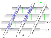
Figure 1: A square metallic network submitted to a magnetic field. Schematic picture of a closed diffusive trajectory winding a flux $2\phi$ is represented ($\phi$ is the flux per elementary plaquette).

(ii) e-e interaction leads to geometry dependent decoherence.– Not only the winding probability $\mathcal{P}_{n}(t)$ involved in eq. (2) is affected by the nontrivial topology of networks, but also $\langle{\mbox{\large e}}^{\mathrm{i}\Phi(t)}\rangle={\mbox{\large e}}^{-t/\tau_{\varphi}}$ describing the nature of phase coherence relaxation is replaced by a more complex function. When decoherence is due to e-e interaction, the dominant phase-breaking mechanism at low temperature, this relaxation is not described by a simple exponential anymore. This situation will be refered as model B throughout this paper. Such decoherence can be modeled in a one-electron picture by including dephasing due to the fluctuating electromagnetic field created by the other electrons AltAroKhm82 . Therefore the pair of reversed interfering trajectories picks up an additional phase $\Phi[\mathcal{C}]$ that depends on the electric potential $V$. Averaging over the fluctuations of the potential leads to the relaxation of phase coherence. The harmonics present the structure

$$\Delta\sigma_{n}\sim-\int_{0}^{\infty}\mathrm{d}{t}\,\mathcal{P}_{n}(t)\>\langle{\mbox{\large e}}^{\mathrm{i}\Phi[\mathcal{C}_{t}^{n}]}\rangle_{V,\mathcal{C}_{t}^{n}}\>,$$ (4)

where averaging is taken over the potential fluctuations $\langle\cdots\rangle_{V}$ and over the loops with winding $n$ for time $t$, $\langle\cdots\rangle_{\mathcal{C}_{t}^{n}}$. In a quasi 1d-wire, the relaxation of phase coherence involves an important length scale, the Nyquist length $L_{N}$, characterizing the efficiency of the electron-electron interaction to destroy the phase coherence in the wire. We will see that, in networks also, the Nyquist length is the intrinsic length characterizing decoherence due to e-e interaction. It is given by AltAroKhm82 ; AltAro85 ; footnote3 ; footnote4

$$\boxed{L_{N}=\left(\frac{\hbar^{2}\sigma_{0}Ds}{e^{2}k_{B}T}\right)^{1/3}=\left(\frac{\alpha_{d}}{\pi}N_{c}\ell_{e}L_{T}^{2}\right)^{1/3}}$$ (5)

where $s$ is the cross-section of the wire. We have rewritten the Nyquist length in terms of the thermal length $L_{T}=\sqrt{\hbar{}D/k_{B}T}$, the elastic mean free path $\ell_{e}$ and the number of conducting channels $N_{c}$ (not including spin degeneracy) ; $\alpha_{d}$ is a dimensionless constant depending on the dimension ($\alpha_{d}=V_{d}/V_{d-1}$ where $V_{d}$ is the volume of the unit sphere in dimension $d$) footnote5 . In the following we will set $\hbar=k_{B}=1$. In the infinite wire, the decaying function $\langle{\mbox{\large e}}^{\mathrm{i}\Phi}\rangle_{V,\mathcal{C}_{t}}$ can only involve the unique length $L_{N}$. A precise analysis of the magnetoconductance (MC) of the wire shows that, in this case, the calculation of (2) and (4) for the infinite wire, for which $\mathcal{P}(t)\propto 1/\sqrt{t}$, leads to almost indistinguishable results provided Pie00 ; AkkMon07 $L_{\varphi}\to\sqrt{2}\,L_{N}$. Therefore the analysis of the MC of the wire suggests that the sophisticated calculation of (4) can be replaced by the simpler one (2) with ${\mbox{\large e}}^{-t/\tau_{\varphi}}\to{\mbox{\large e}}^{-t/2\tau_{N}}$ where $\tau_{N}=L_{N}^{2}/D\propto{}T^{-2/3}$ is the Nyquist time. However this is a priori not true anymore as soon as we consider networks with a nontrivial topology because electric potential fluctuations depend on the geometry, and therefore the decoherence is geometry-dependent.

Let us formulate this idea more precisely. Being related to the potential as $\Phi\sim\int^{t}V$, fluctuations of the phase $\Phi$ picked by the two reversed electronic trajectories can be related to the power spectrum of the potential, given by the fluctuation-dissipation theorem (FDT) : $\frac{\mathrm{d}}{\mathrm{d}{}t}\langle\Phi^{2}\rangle_{V,\,\mathcal{C}_{t}}\sim{}e^{2}T\mathcal{R}_{t}\sim\frac{e^{2}T}{\sigma_{0}s}x(t)$ where $\mathcal{R}_{t}=x(t)/(\sigma_{0}s)$ is the resistance of a wire of length $x(t)$. The average $\langle\cdots\rangle_{V,\,\mathcal{C}_{t}}$ is taken over potential fluctuations and closed diffusive trajectories $\mathcal{C}_{t}$ for a time scale $t$. The length $x(t)$ is the typical length probed by electronic trajectories. For an infinite wire it scales like $x(t)\sim\sqrt{Dt}$ therefore $\langle\Phi^{2}\rangle_{V,\,\mathcal{C}_{t}}\sim(t/\tau_{N})^{3/2}$ where $\tau_{N}=L_{N}^{2}/D\sim{T}^{-2/3}$ is the Nyquist time. On the other hand, in a ring, diffusion is constrained by the geometry : harmonics of the MC of a ring involve winding trajectories for which the length scale probed is therefore the perimeter $x(t)\sim{L}$, leading to $\langle\Phi^{2}\rangle_{V,\,\mathcal{C}_{t}}\sim(t/\tau_{c})$ where $\tau_{c}\sim{T}^{-1}$. Therefore, in a ring, depending on their winding, trajectories probe different length scales : $L_{N}\propto{T}^{-1/3}$ or $L_{c}\propto{T}^{-1/2}$.

Let us summarize. At the level of eqs. (2,3), $L_{\varphi}$ is a phenomenological parameter put by hand. The modelization of decoherence due to e-e interaction of AAK shows that, in an infinite wire, the WL correction probes the Nyquist length $L_{N}\propto{T}^{-1/3}$ (the only length scale of the problem). This shows that, in the MC of the infinite wire, the phenomenological parameter $L_{\varphi}$ must be replaced by $L_{\varphi}\to{}L_{N}\propto{T}^{-1/3}$. On the other hand the MC of a ring involves a new length scale $L_{c}=L_{N}^{3/2}/L^{1/2}$ combination of the Nyquist length and the perimeter. In this case, assuming the simple AAS behaviour $\Delta\sigma_{n}\propto{\mbox{\large e}}^{-nL/L_{\varphi}}$, the phenomenological parameter should be substituted by $L_{\varphi}\to{}L_{c}\propto{T}^{-1/2}$.

Geometry dependent decoherence in ballistic rings.– It is worth pointing that such a geometry dependent decoherence can also be observed in ballistic systems : potential fluctuations responsible for decoherence depend on the precise distribution of currents inside the device, that are affected by the way the current is injected through different contacts PedLanBut98 . Depending whether the measurement is local or nonlocal, different phase coherence lengths have been extracted from the damping of AB oscillations KobAikKatIye02 . The different $\tau_{\varphi}$ are probed by changing the contact configuration (current/voltage probes) SeePilJorBut03 , whereas in the diffusive ring, the different length scales are probed by considering different harmonics.

III General formalism

We first recall the basic formalism and apply precisely the ideas given in the introduction. We will consider the reduced conductivity $\tilde{\sigma}$, defined by

$$\sigma=\frac{2e^{2}}{h\,s}\,\tilde{\sigma}$$ (6)

where $s$ is the cross-section of the wire. The reduced WL correction has the dimension of a length. As mentioned above, it is a sum of contributions of interfering closed reversed electronic trajectories, which can be conveniently written as a path integral :

$$\Delta\tilde{\sigma}(x)\equiv-2\,P_{c}(x,x)$$ (7)

$$=-2\int_{0}^{\infty}\mathrm{d}{t}\,\int_{x(0)=x}^{x(t)=x}\mathcal{D}x(\tau)\,{\mbox{\large e}}^{-\int_{0}^{t}\mathrm{d}\tau\,\big{(}\frac{1}{4}\dot{x}^{2}+2\mathrm{i}{e}\dot{x}A(x)\big{)}}\,{\mbox{\large e}}^{\mathrm{i}\Phi[x(\tau)]}\>.$$

$P_{c}(x,x)$ is the so-called Cooperon. Summation over diffusive paths for time $t$ involves the Wiener measure $\mathcal{D}x(\tau)\exp{-\int_{0}^{t}\mathrm{d}\tau\,\frac{1}{4}\dot{x}^{2}}$ (we have performed a change of variable $t\to{}t/D$ so that “time” has now the dimension of a squared length). Each loop receives a phase proportional to the magnetic flux $2\int_{0}^{t}\mathrm{d}\tau\,\dot{x}A(x)$ intercepted by the reversed interfering trajectories, where $A(x)$ is the vector potential. The factor $2$ originates from the fact that the Cooperon measures interference between two closed electronic trajectories undergoing the same sequence of scattering events in a reversed order. Finally we have introduced an additional phase $\Phi[x(\tau)]$ to account for dephasing : dephasing due to penetration of the magnetic field in the wires AltAro81 or decoherence due to electron-electron interaction. In this latter case the phase $\Phi$ depends also on the environment dynamics over which one should average.

The $x$ dependence of $\Delta\tilde{\sigma}(x)$ in eq. (7).– In a general network, in the absence of translational invariance, the WL correction to the conductance was shown to be given by an integration of $\Delta\tilde{\sigma}(x)$ over the network, with some nontrivial weights attributed to the wires. Let us write the classical dimensionless conductance as $g^{\mathrm{class}}=\alpha_{d}N_{c}\ell_{e}/\mathcal{L}$ where the effective length $\mathcal{L}$ is obtained from addition (Kirchhoff) laws of classical resistances (dimensionless parameter $\alpha_{d}$ was defined above : $\alpha_{3}=4/3$, $\alpha_{2}=\pi/2$ and $\alpha_{1}=2$). Then the WL correction to the conductance is TexMon04

$$\Delta{}g=\frac{1}{\mathcal{L}^{2}}\sum_{i}\frac{\partial\mathcal{L}}{\partial l_{i}}\,\int_{\mathrm{wire}\>i}\mathrm{d}x\,\Delta\tilde{\sigma}(x)\>,$$ (8)

where the summation runs over all wires of the networks and $l_{i}$ is the length of the wire $i$. Eq. (8) was demonstrated in Ref. TexMon04 for the conductance matrix elements of multiterminal networks with arbitrary topology. This result relies on a careful discussion of current conservation (derivation of current conserving quantum corrections can be found in Refs. KanSerLee88 ; HerAmb88 ; Her89 ; HasStoBar94 ). This point will play a relatively minor role in the present paper. Eq. (8) may be used in order to calculate geometry dependent prefactors.

Magnetoconductance oscillations and winding properties.– In an array of metallic rings of same perimeter, the magnetic flux is an integer multiple of the flux $\phi$ per ring $\int_{0}^{t}\mathrm{d}\tau\,\dot{x}A(x)=\phi\times\mathcal{N}[x(\tau)]$ where $\mathcal{N}[x(\tau)]\in{\ensmathonze Z}$ is the winding number of the closed trajectory (the number of fluxes encircled). This makes the WL correction a periodic function of the flux $\phi=\theta\frac{\phi_{0}}{4\pi}$, where $\phi_{0}=h/e$. The $n$-th harmonic of the MC

$$\Delta\tilde{\sigma}_{n}=\int_{0}^{2\pi}\frac{\mathrm{d}\theta}{2\pi}\Delta\tilde{\sigma}(\theta)\>{\mbox{\large e}}^{-\mathrm{i}{n}\theta}$$ (9)

involves trajectories with winding number $n$. We can write the harmonics as

$$\Delta\tilde{\sigma}_{n}(x)\equiv-2\,P_{c}^{(n)}(x,x)=-2\,\int_{0}^{\infty}\mathrm{d}{t}\,$$ (10)

$$\times\int_{x(0)=x}^{x(t)=x}\mathcal{D}x(\tau)\,\delta_{n,\mathcal{N}[x(\tau)]}\,{\mbox{\large e}}^{-\int_{0}^{t}\mathrm{d}\tau\,\frac{1}{4}\dot{x}^{2}}\,{\mbox{\large e}}^{\mathrm{i}\Phi[x(\tau)]}\>,$$

where the Kronecker symbol selects only trajectories for a given winding number $n$. Let us introduce the probability for a diffusive particle to return to its starting point after a time $t$, with the condition of winding $n$ fluxes

$$\mathcal{P}_{n}(x,x;t)=\int_{x(0)=x}^{x(t)=x}\mathcal{D}x(\tau)\,\delta_{n,\mathcal{N}[x(\tau)]}\,{\mbox{\large e}}^{-\int_{0}^{t}\mathrm{d}\tau\,\frac{1}{4}\dot{x}^{2}}\>.$$ (11)

For example, in an isolated ring of perimeter $L$, this probability is simply given by

$$\mathcal{P}_{n}^{\mathrm{ring}}(x,x;t)=\frac{1}{\sqrt{4\pi{t}}}\,{\mbox{\large e}}^{-\frac{(nL)^{2}}{4t}}\>.$$ (12)

Then, we can rewrite the harmonics as

$$\boxed{\Delta\tilde{\sigma}_{n}(x)=-2\,\int_{0}^{\infty}\mathrm{d}{t}\,\mathcal{P}_{n}(x,x;t)\,\langle{\mbox{\large e}}^{\mathrm{i}\Phi[\mathcal{C}^{n}_{t}]}\rangle_{\mathcal{C}^{n}_{t}}}\>,$$ (13)

which is the structure given in eq. (4). In eq. (13) we have introduced the notation $\mathcal{C}^{n}_{t}\equiv(x(\tau),\,\tau\in[0,t]\,|\,x(0)=x(t)=x\,;\,\mathcal{N}[x(\tau)]=n)$ for a closed diffusive path winding $n$ times. $\left\langle\cdots\right\rangle_{\mathcal{C}^{n}_{t}}$ designates averaging over all such paths, with the measure of the path integral (11). The phase $\Phi[\mathcal{C}]$ accounts for dephasing and eliminates the contributions of diffusing trajectories at large time. We now discuss two possible modelizations for this function, denoted by “A” and “B”.

III.1 Model A : Exponential relaxation

The simplest choice is an exponential relaxation, with a dephasing rate $\gamma=1/\tau_{\varphi}=1/L_{\varphi}^{2}$ :

$$\langle{\mbox{\large e}}^{\mathrm{i}\Phi[\mathcal{C}_{t}]}\rangle_{\mathcal{C}_{t}}={\mbox{\large e}}^{-\gamma t}\>.$$ (14)

This simple prescription correctly describes dephasing due to spin-orbit coupling, magnetic impurities HikLarNag80 ; Ber84 , effect of penetration of the magnetic field in the wires AltAro81 , or decoherence due to electron-phonon scattering ChaSch86 ; footnote6 . Using (12,13) with this exponential decay yields the familiar result (3) for the isolated ring.

III.2 Model B : geometry dependent decoherence from electron-electron interaction

It turns out that the simple exponential relaxation does not describe correctly the decoherence due to electron-electron interaction, the physical reason being that this decoherence is due to electromagnetic field fluctuations that depend on the geometry of the system. AAK have proposed a microscopic description AltAroKhm82 ; AltAro85 that we can rephrase as follows. In eq. (7), the phase $\Phi$ picked up by the reversed trajectories depends on the environment (the potential $V$ created by the other electrons due to electron-electron interaction) : $\Phi_{V}[\mathcal{C}_{t}]=\int_{0}^{t}\mathrm{d}\tau\,[V(x(\tau),\tau)-V(x(\tau),t-\tau)]$. Averaging over the Gaussian fluctuations of $V$ leads to $\langle{\mbox{\large e}}^{\mathrm{i}\Phi_{V}[\mathcal{C}_{t}]}\rangle_{V}={\mbox{\large e}}^{-\frac{1}{2}\langle\Phi_{V}[\mathcal{C}_{t}]^{2}\rangle_{V}}$ where the fluctuation-dissipation theorem (written for $\omega\ll{}T$ describing classical fluctuations) $\langle V(r,t)V(r^{\prime},t^{\prime})\rangle_{V}\simeq\frac{e^{2}T}{\sigma_{0}}\delta(t-t^{\prime})\,P_{d}(r,r^{\prime})$ gives $\frac{1}{2}\langle\Phi_{V}[\mathcal{C}_{t}]^{2}\rangle_{V}=\Gamma[\mathcal{C}_{t}]\,t$ with footnote7

$$\boxed{\Gamma[\mathcal{C}_{t}]\,t=\frac{2}{L_{N}^{3}}\int_{0}^{t}\mathrm{d}\tau\,W(x(\tau),x(t-\tau))}$$ (15)

$$=\frac{k_{B}T}{\hbar}\frac{2\pi}{R_{K}}\int_{0}^{t}\mathrm{d}\tau\,\mathcal{R}(x(\tau),x(t-\tau))\>,$$ (16)

where $R_{K}=h/e^{2}$ is the quantum of resistance. The function $W(x,x^{\prime})$ is related to the diffuson, solution of $-\Delta{P_{d}}(x,x^{\prime})=\delta(x-x^{\prime})$, by

$$W(x,x^{\prime})=\frac{P_{d}(x,x)+P_{d}(x^{\prime},x^{\prime})}{2}-P_{d}(x,x^{\prime})\>.$$ (17)

This function has a physical interpretation discussed in the appendix E : it is proportional to the equivalent resistance $\mathcal{R}(x,x^{\prime})$ between the points $x$ and $x^{\prime}$ (figure 21). With this remark, we see that eq. (16) can be understood as a local version of the Johnson-Nyquist theorem relating the potential fluctuations to the resistance.

In eqs. (15,16) we have introduced a decoherence rate $\Gamma[\mathcal{C}_{t}]$ which depends not only on the time but on the trajectory itself. Therefore the decay of phase coherence is now described by

$$\boxed{\langle{\mbox{\large e}}^{\mathrm{i}\Phi_{V}[\mathcal{C}_{t}]}\rangle_{V,\mathcal{C}_{t}}=\langle{\mbox{\large e}}^{-\Gamma[\mathcal{C}_{t}]\,t}\rangle_{\mathcal{C}_{t}}}\>.$$ (18)

Within this framework, relaxation of phase coherence is not described by a simple exponential decay like in eq. (14) but is controlled by a functional of the trajectories footnote8 $x(\tau)$. Therefore the nature of decoherence depends on the network, through the resistance $\mathcal{R}(x,x^{\prime})$ between $x$ and $x^{\prime}$, and on the winding properties of the trajectories.

The central problem of the present paper is to compute the path integral

$$\Delta\tilde{\sigma}_{n}(x)=-2\,\int_{0}^{\infty}\mathrm{d}{t}\,{\mbox{\large e}}^{-\gamma t}\int_{x(0)=x}^{x(t)=x}\mathcal{D}x(\tau)\,\delta_{n,\mathcal{N}[x(\tau)]}\,$$

$$\hskip 56.9055pt\times{\mbox{\large e}}^{-\int_{0}^{t}\mathrm{d}\tau\,\big{[}\frac{1}{4}\dot{x}^{2}+\frac{2}{L_{N}^{3}}W(x(\tau),x(t-\tau))\big{]}}$$ (19)

for the different networks. Such a calculation has been already performed in two cases : the infinite wire AltAroKhm82 and the isolated ring LudMir04 ; TexMon05b .

The logic of the following sections is the following : first we study the winding properties in the network. For that purpose we first compute the WL correction $\Delta\tilde{\sigma}_{n}^{(A)}$ within model A, eq. (13) with (14). The probability $\mathcal{P}_{n}(x,x;t)$ can be extracted from an inverse Laplace transform with respect to the parameter $\gamma$. Having fully characterized the winding properties, we use this information in order to study the harmonics $\Delta\tilde{\sigma}_{n}^{(B)}$ within the model B describing decoherence due to electron-electron interaction, eq. (13) with (18).

IV The wire and the ring

We first recall known results within the framework of model B concerning the simplest geometries that will be useful for the following.

IV.1 Phase coherence relaxation in an infinite wire

The case of an infinite wire was originally solved in Ref. AltAroKhm82 . In this case we have $W_{\mathrm{wire}}(x,x^{\prime})=\frac{1}{2}|x-x^{\prime}|$ and the path integral

$$\Delta\tilde{\sigma}= -2\int_{0}^{\infty}\mathrm{d}{t}\,{\mbox{\large e}}^{-\gamma t}$$ (20)

$$\times\int_{x(0)=x}^{x(t)=x}\mathcal{D}x(\tau)\,{\mbox{\large e}}^{-\int_{0}^{t}\mathrm{d}\tau\,\big{[}\frac{1}{4}\dot{x}^{2}+\frac{1}{L_{N}^{3}}|x(\tau)-x(t-\tau)|\big{]}}$$

can be computed thanks to translational invariance (as pointed in Ref. ComDesTex05 , using the symmetry of the path integral we can perform the substitution $x(\tau)-x(t-\tau)\to{}x(\tau)$, provided that the starting point of the path integral is set to $x\to 0$, see appendix A). Combining exponential relaxation (model A) and decoherence due to e-e interaction (model B) allows to extract the function (18) with an inverse Laplace transform of the AAK result AltAroKhm82 ; AltAro85 ; AleAltGer99 ; AkkMon07

$$\Delta\tilde{\sigma} =-\int_{0}^{\infty}\frac{\mathrm{d}{t}}{\sqrt{\pi{}t}}\,{\mbox{\large e}}^{-\gamma t}\,\langle{\mbox{\large e}}^{\mathrm{i}\Phi_{V}[\mathcal{C}_{t}]}\rangle_{V,\mathcal{C}_{t}}$$ (21)

$$=L_{N}\frac{\mathrm{Ai}(\gamma\,L_{N}^{2})}{\mathrm{Ai}^{\prime}(\gamma\,L_{N}^{2})}\>,$$ (22)

where $\mathrm{Ai}(z)$ is the Airy function AbrSte64 . As mentioned above, this expression is very close to Pie00 ; AkkMon07 $\Delta\tilde{\sigma}\simeq-\big{(}\frac{1}{L_{\varphi}^{2}}+\frac{1}{2L_{N}^{2}}\big{)}^{-1/2}$, the result obtained by performing the substitution $\langle{\mbox{\large e}}^{\mathrm{i}\Phi_{V}[\mathcal{C}_{t}]}\rangle_{V,\mathcal{C}_{t}}\to{\mbox{\large e}}^{-t/2L_{N}^{2}}$ (see figure 2).

The inverse Laplace transform of (21) was computed in Ref. MonAkk05 with residue’s theorem :

$$f_{\mathrm{wire}}\left({t}/{\tau_{N}}\right) =\langle{\mbox{\large e}}^{\mathrm{i}\Phi_{V}[\mathcal{C}_{t}]}\rangle_{V,\mathcal{C}_{t}}$$ (23)

$$=\sqrt{\frac{\pi t}{\tau_{N}}}\sum_{m=1}^{\infty}\frac{1}{|u_{m}|}{\mbox{\large e}}^{-|u_{m}|t/\tau_{N}}\>,$$ (24)

where $u_{m}$ are zeros of $\mathrm{Ai}^{\prime}(z)$. In particular $u_{1}\simeq-1.019$ and $u_{m}\simeq-[\frac{3\pi}{2}(m-\frac{3}{4})]^{2/3}$ for $m\to\infty$. The limiting behaviours are

$$f_{\mathrm{wire}}\left({t}/{\tau_{N}}\right) \simeq 1-\frac{\sqrt{\pi}}{4}\,\left(\frac{t}{\tau_{N}}\right)^{3/2}\hskip 14.22636pt\mbox{for }t\ll\tau_{N}$$ (25)

$$\simeq\frac{1}{|u_{1}|}\sqrt{\frac{\pi t}{\tau_{N}}}\,{\mbox{\large e}}^{-|u_{1}|t/\tau_{N}}\hskip 9.95863pt\mbox{for }\tau_{N}\ll t\>.$$ (26)

Note that the short time behaviour can be obtained by expanding $f\left({t}/{\tau_{N}}\right)=\langle{\mbox{\large e}}^{\mathrm{i}\Phi}\rangle_{V,\mathcal{C}_{t}}=\langle{\mbox{\large e}}^{-\frac{1}{2}\langle\Phi^{2}\rangle_{V}}\rangle_{\mathcal{C}_{t}}\simeq 1-\frac{1}{2}\langle\Phi_{V}[\mathcal{C}_{t}]^{2}\rangle_{V,\mathcal{C}_{t}}$. This limit can be simply obtained by noticing that in the wire $W(x(\tau),x(t-\tau))\sim{}x(\tau)\sim\sqrt{t}$, therefore $\Gamma[\mathcal{C}_{t}]\,t\sim{}T\,t^{3/2}\sim({t}/{\tau_{N}})^{3/2}$ where we recover that the Nyquist time scales as $\tau_{N}\propto{}T^{-2/3}$.

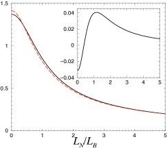
Figure 2: Comparison between $-\mathrm{Ai}(x^{2})/\mathrm{Ai}^{\prime}(x^{2})$ (black continuous line) and $1/\sqrt{1/2+x^{2}}$ (red dashed line). Relative difference (inset) does not exceed 4%.

IV.2 Phase coherence relaxation in the isolated ring

For the isolated ring of perimeter $L$, we have $W_{\mathrm{ring}}(x,x^{\prime})=\frac{1}{2}|x-x^{\prime}|(1-\frac{|x-x^{\prime}|}{L})$. The path integral (III.2) can be computed exactly TexMon05b (see appendix A). Up to a dimensionless prefactor, we obtain

$$\Delta\tilde{\sigma}_{n} \sim-L_{N}\,{\mbox{\large e}}^{-\frac{\pi}{8}n(L/L_{N})^{3/2}}\hskip 14.22636pt\mbox{for }L_{N}\ll L$$ (27)

$$\sim-T^{-1/3}\,{\mbox{\large e}}^{-nL^{3/2}T^{1/2}}\>.$$ (28)

This result can be simply understood as follows : in the ring, trajectories with finite winding necessarily explore the whole ring. This “ergodicity” implies that $W(x(\tau),x(t-\tau))\sim{}x(\tau)\sim{}L$ and therefore the decoherence rate $\Gamma[\mathcal{C}_{t}]\,t\sim{}TL\,t\sim{t}/{\tau_{c}}$ involves the different time scale $\tau_{c}\sim 1/(TL)$, according to the physical argument given in section II. As a consequence Eq. (13) indeed leads to LudMir04

$$\Delta\tilde{\sigma}_{n}\sim-L_{N}\,{\mbox{\large e}}^{-\frac{\pi}{8}nL/L_{c}}\>,$$ (29)

where

$$\boxed{L_{c}=\frac{L_{N}^{3/2}}{L^{1/2}}}\>.$$ (30)

Figure 3: The relative difference ($1-\eta(x^{2})/\sqrt{(\pi/8)^{2}+x^{2}}$) between the effective length $L_{\varphi}^{\mathrm{osc}}$, eq. (33), and its approximation, eq. (36), does not exceed 1.5%.

Phase coherence length : $L_{\varphi}\propto{}T^{-1/3}$ or $L_{\varphi}\propto{}T^{-1/2}$ ?– Note that the introduction of a new length scale LudMir04 $L_{c}$ might appear arbitrary since the harmonics may be written uniquely in terms TexMon05b of $L$ and $L_{N}$. The difference between (27) and (29) is a matter of convention and may be related to the experimental procedure. The usual method extracts the phase coherence length from the analysis of MC harmonics. Then it is natural to see how the winding number $n$ scales with the phase coherence length, or more properly how the length $nL$ scales with $L_{\varphi}$ and therefore assume the form $\Delta\tilde{\sigma}_{n}\propto{}f(nL/L_{\varphi})$. From eq. (29) we see that the function is simply the exponential, $f(x)={\mbox{\large e}}^{-x}$, with a perimeter dependent phase coherence length $L_{\varphi}\to{L_{c}}\propto{}(TL)^{-1/2}$. Another procedure may consist in studying the harmonics content as a function of the perimeter $L$, that is for different samples. The experiment is then analyzed with the form $\Delta\tilde{\sigma}_{n}\propto{}f_{n}(L/L_{\varphi})$. Eq. (27) gives $f_{n}(x)={\mbox{\large e}}^{-nx^{3/2}}$ with the geometry independent phase coherence length $L_{\varphi}\to{L_{N}}\propto{}T^{-1/3}$.

The temperature dependence $\Delta\sigma_{n}\sim{\mbox{\large e}}^{-L^{3/2}T^{1/2}}$ was first predicted in Ref. LudMir04 using instanton method (with a different pre-exponential dependence) and studied in details in Ref. TexMon05b where the path integral (III.2) was computed exactly for the isolated ring. The effect of the connecting arms was clarified in Ref. Tex07b . The fact that the pre-exponential factor is $L_{N}$ is related to the fact that the smooth part of the MC, due to the penetration of the field in the wire, probes the same length scale as in the infinite wire.

It is worth pointing the recent work TreYevMarDelLer09 in which the crossover to the 0d limit is studied in a ring weakly connected. In this case the authors get a crossover from $\tau_{\varphi}\propto{}T^{-1}$ (diffusive ring) to $\tau_{\varphi}\propto{}T^{-2}$ (ergodic) for temperature below the Thouless energy. This latter behaviour coincides with the result known for quantum dots in the same regime SivImrAro94 .

IV.3 Penetration of the magnetic field in the wires of the ring

Networks are made of wires of finite width $w$. The penetration of the magnetic field in the wires is responsible for fluctuations of the magnetic flux enclosed by trajectories with the same winding number but different areas. In the weak magnetic field limit, this effect is described by introducing an effective dephasing rate AltAro81

$$\gamma\to 1/L_{\mathcal{B}}^{2}=\frac{1}{3}\left(\frac{e\mathcal{B}w}{\hbar}\right)^{2}\>.$$ (31)

The question of how to combine the two decoherence mechanisms (models A & B) in the ring was discussed in Ref. TexMon05b . It was shown that the WL correction of the ring presents the structure

$$\Delta\tilde{\sigma}_{n}\simeq L_{N}\,\frac{\mathrm{Ai}(L_{N}^{2}/L_{\mathcal{B}}^{2})}{\mathrm{Ai}^{\prime}(L_{N}^{2}/L_{\mathcal{B}}^{2})}\,{\mbox{\large e}}^{-nL/L_{\varphi}^{\mathrm{osc}}(L_{c},L_{\mathcal{B}})}$$ (32)

for $L_{N}\ll L$, with

$$L_{\varphi}^{\mathrm{osc}}(L_{c},L_{\mathcal{B}})=\frac{L_{c}}{\eta(L_{c}^{2}/L_{\mathcal{B}}^{2})}\>,$$ (33)

where $\eta(x)=(\frac{1}{4}+x)\arctan\frac{1}{2\sqrt{x}}+\frac{\sqrt{x}}{2}$.

Prefactor.– In eq. (32), the pre-exponential factor coincides with the result obtained for an infinite wire AltAroKhm82 . The ratio of Airy functions can be approximated as Pie00 ; AkkMon07 $\frac{\mathrm{Ai}(x)}{\mathrm{Ai}^{\prime}(x)}\simeq-(\frac{1}{2}+x)^{-1/2}$ (figure 2). In other terms, we may write the zero harmonic (i.e. the result for the infinite wire) as

$$\Delta\tilde{\sigma}_{0}\simeq-L_{\varphi}^{\mathrm{env}}$$ (34)

where

$$L_{\varphi}^{\mathrm{env}}=\left(\frac{1}{2L_{N}^{2}}+\frac{1}{L_{\mathcal{B}}^{2}}\right)^{-1/2}\>.$$ (35)

This combination expresses that, in a wire of width $w$, the penetration of the magnetic field provides the dominant cutoff when typical trajectories enclose more than one quantum flux $L_{\varphi}{}w\mathcal{B}\gtrsim\phi_{0}$ (here $L_{\varphi}\sim{}L_{N}$ for trajectories with winding $n=0$).

Exponential damping.– In the exponential of eq. (32), the effective length interpolates between $L_{\varphi}^{\mathrm{osc}}\simeq\frac{8}{\pi}{L_{c}}$ for $L_{\mathcal{B}}\gg{L_{c}}$ and $L_{\varphi}^{\mathrm{osc}}\simeq{}L_{\mathcal{B}}$ for $L_{\mathcal{B}}\ll{L_{c}}$. Its overall behaviour is well approximated by

$$L_{\varphi}^{\mathrm{osc}}\simeq\left[\left(\frac{\pi}{8L_{c}}\right)^{2}+\frac{1}{L_{\mathcal{B}}^{2}}\right]^{-1/2}=\left(\frac{\pi^{2}L}{64L_{N}^{3}}+\frac{1}{L_{\mathcal{B}}^{2}}\right)^{-1/2}$$ (36)

which differs with (33) by less than 1.5% (figure 3). When $L_{\mathcal{B}}$ is the shortest length, the decay of AAS oscillations $\sim{\mbox{\large e}}^{-nL/L_{\mathcal{B}}}$ can be understood from the fact that modulations of the flux enclosed by trajectories with finite winding become larger than the quantum flux $nLw\mathcal{B}\gtrsim\phi_{0}$. Eq. (36) was used in the analysis of the recent experiment FerRowGueBouTexMon08 .

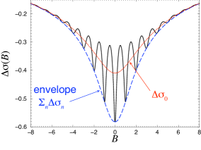
Figure 4: Typical shape of the MC curve of a network (here a chain of rings). Rapid oscillations are AAS oscillations. Damping of oscillations over large scale is due to the penetration of the magnetic field in the wires.

These two remarks show that the magnetic length $L_{\mathcal{B}}$ probes two different length scales : in the pre-exponential factor $L_{\mathcal{B}}$ probes the Nyquist length $L_{N}\propto{T}^{-1/3}$, whereas in the ratio of harmonics $\Delta\tilde{\sigma}_{n}/\Delta\tilde{\sigma}_{0}$, the magnetic length $L_{\mathcal{B}}$ probes the length scale $L_{c}\propto{T}^{-1/2}$.

IV.4 How to analyze MC experiments in networks

In order to understand the implications of this remark, let us discuss the structure of the typical MC curve of a network. The following discussion applies to the case $L_{N}\lesssim{}L$ where (32) holds. Figure 4 represents a typical MC curve, here for a chain of rings. It exhibits rapid AAS oscillations with a period given by $\mathcal{B}_{\mathrm{osc}}\sim\phi_{0}/L^{2}$, superimposed with a smooth variation over a scale $\mathcal{B}_{\mathrm{damp}}\sim\phi_{0}/wL_{\varphi}$. The phase coherence length can be extracted either from the amplitude of the oscillations or from the decay of the envelope of the MC curve. Which $L_{\varphi}$ ($L_{N}$ or $L_{c}$) is obtained from such a curve ?

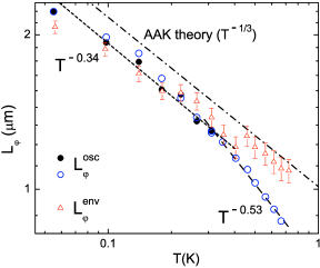
Figure 5: Phase coherence length as a function of the temperature obtained from measurements realized on a large square network FerRowGueBouTexMon08 of lattice spacing $a=1\>\mu$m (perimeter $L=4\>\mu$m). The length scale $L_{\varphi}\to{}L_{\varphi}^{\mathrm{env}}\propto{T}^{-1/3}$ has been extracted from the smooth MC while the length $L_{\varphi}\to{}L_{\varphi}^{\mathrm{osc}}\propto{T}^{-1/2}$ has been extracted from ratio of harmonics. (Note that $L_{\varphi}^{\mathrm{env}}$ and $L_{\varphi}^{\mathrm{osc}}$ in Ref. FerRowGueBouTexMon08 denote eqs. (35) and (36) for $L_{\mathcal{B}}=\infty$).

According to (32) we see that $L_{\varphi}\to{}L_{N}$ in the pre-exponential factor, which mostly dominates the smooth envelope, while $L_{\varphi}\to{}L_{c}$ in the exponential decay, which dominates the damping of the rapid oscillations. In order to decouple the two effects the analysis of the experiments of Ref. FerRowGueBouTexMon08 have been analyzed as follows Fer04 ; FerAngRowGueBouTexMonMai04  : the Fourier transform of the MC curve $\Delta\sigma(\mathcal{B})$ presents broadened Fourier peaks due to the penetration of the magnetic field in the wires. Integration of Fourier peaks eliminates this effect. Ratio of harmonics involve the length scale $L_{c}$. The length $L_{N}$ was extracted from the smooth envelope $\Delta\tilde{\sigma}_{\mathrm{env}}=\sum_{n}\Delta\tilde{\sigma}_{n}\simeq\Delta\tilde{\sigma}_{0}$ for $L_{N}\ll{}L$. The temperature dependence of the phase coherence length was extracted in this way in Ref. FerRowGueBouTexMon08 . Results are plotted on figure 5, exhibiting clearly the two length scales in the regime $L_{N}\ll{}L$. We see that it is crucial to analyze the experiment in terms of the MC harmonics $\Delta\sigma_{n}$.

Isolated ring vs ring embedded in a network.– In transport experiments the ring is never isolated : it is at least connected to contacts through which current is injected. Moreover the samples are often made of a large number of loops, in order to realize disorder averaging. The results obtained for the isolated ring are fortunately relevant to describe a more complex network of equivalent rings (Figs. 1 & 9) when the rings can be considered as independent, i.e. when interference phenomena do not involve several rings ; this occurs when $L_{\varphi}\ll{L}$ (or $L_{N}\ll{L}$), in practice in a high temperature regime. This temperature dependence of harmonics is rather difficult to extract from measurements since harmonics are suppressed exponentially. This has been done only very recently in Ref. FerRowGueBouTexMon08 . Another difficulty is that the “high temperature regime” $L_{N}\ll{}L$ is in practice quite narrow in these samples due to fact that electron-phonon interaction dominates the decoherence above $1\>$K (in the sample of Refs. SchMalMaiTexMonSamBau07 ; Mal06 $L_{N}$ is much larger and when $L_{N}\ll{}L$ the role of electron-eletron interaction is negligible).

It is an important issue to obtain the expression of the WL correction for a broader temperature range, that is to study the regime $L\lesssim{}L_{N}$. This regime is reached in several experiments FerAngRowGueBouTexMonMai04 ; SchMalMaiTexMonSamBau07 ; Mal06 . In this case diffusive interfering trajectories responsible for AAS harmonics are not constrained to remain inside a unique ring, but explore the surrounding network (see figs. 1, 6 & 9). This affects both the winding properties and the nature of decoherence. The MC oscillations are therefore network dependent. In the following sections we discuss the behaviour of the MC harmonics in the limit $L\lesssim{}L_{\varphi}$ (or $L\lesssim{}L_{N}$) for different networks : a ring connected to long arms, a necklace of rings and a large square network. The case of a long hollow cylinder will also be discussed.

V The connected ring

In this section we consider the case of a single ring connected to two wires supposed much longer than $L_{\varphi}$ (figure 6). This problem has already been considered in Refs. TexMon05 ; TexMon05b .

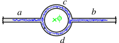
Figure 6: A ring connected to reservoirs through long wires $a$ and $b$. In the regime $L_{\varphi}\gtrsim{}L$, the WL correction is dominated by trajectories exploring the arms, as represented here.

V.1 Model A

$\bullet$ Let us consider first the case $L_{\varphi}\ll{}L$. The Cooperon is constructed in appendix F.1 (see Ref. TexMon05 ) and we obtain

$$\Delta\tilde{\sigma}_{n}(x\in\>\mbox{ring})\simeq-\left(\frac{2}{3}\right)^{2n}L_{\varphi}\>{\mbox{\large e}}^{-nL/L_{\varphi}}\>,$$ (37)

where $x$ is any position inside the ring far from the vertices (at distance larger than $L_{\varphi}$).
$\bullet$ Now we turn to the regime $L_{\varphi}\gg{}L$. The Cooperon is uniform inside the ring and is computed in appendix F.1. We have TexMon05  :

$$\Delta\tilde{\sigma}_{n}(x)\simeq-\sqrt{\frac{L_{\varphi}L}{2}}\,{\mbox{\large e}}^{-n\sqrt{2L/L_{\varphi}}}\hskip 14.22636pt\mbox{for }L\ll L_{\varphi}$$ (38)

where $x$ is any position inside the ring, or in the arms at a distance to the ring smaller than $L_{\varphi}$. We emphasize that this behaviour, quite different from (3), is due to the fact that the diffusive trajectories spend most of the time in the wires TexMon05 (the distribution of the time spent by winding trajectories in the arm was analyzed in Ref. ComDesTex05 ).

Winding probability in a ring connected to $N_{a}$ arms.– We now derive the winding probability for a ring connected to $N_{a}$ infinitely long arms (figure 7) from the inverse Laplace transform of the Cooperon $P_{c}^{(n)}(x,x)=-\frac{1}{2}\Delta\tilde{\sigma}_{n}(x)$. At small time, (37) gives

$$\mathcal{P}_{n}(x,x;t)\simeq\left(\frac{2}{3}\right)^{N_{a}n}\frac{1}{\sqrt{4\pi{t}}}\,{\mbox{\large e}}^{-\frac{(nL)^{2}}{4t}}\hskip 7.11317pt\mbox{for }t\ll L^{2}\>,$$ (39)

where $x$ is inside the ring, far from a vertex (at distance larger than $\sqrt{t}$).

At large time scales, $t\gg{}L^{2}$, the arms strongly modify the winding properties around the ring : the time dependence of the typical winding number becomes subdiffusive $n_{t}\sim{t}^{1/4}$, to be compared with the behaviour for the isolated ring $n_{t}\sim{t}^{1/2}$ reflected by eq. (12). For a ring connected to $N_{a}$ infinite wires, eq. (12) is replaced by the probability TexMon05

$$\boxed{\mathcal{P}_{n}(x,x;t)\simeq\frac{\sqrt{L/N_{a}}}{2\,t^{3/4}}\ \Psi\!\left(\frac{n\sqrt{N_{a}L}}{t^{1/4}}\right)\hskip 14.22636pt\mbox{for }t\gg L^{2}}\>,$$ (40)

where $N_{a}$ is the number of arms (as far as $x$ is inside the ring or at a distance to the ring smaller than $t^{1/2}\sim{}1/\sqrt{\gamma}=L_{\varphi}$, the Cooperon, or the corresponding probability is almost independent on $x$). The function $\Psi(\xi)$, given by TexMon05 ; ComDesTex05

$$\Psi(\xi)=\frac{2}{\pi}\mathop{\mathrm{Re}}\nolimits\left[{\mbox{\large e}}^{-\mathrm{i}\frac{\pi}{4}}\int_{0}^{\infty}\mathrm{d}{u}\,\sqrt{u}\,{\mbox{\large e}}^{-u^{2}-\sqrt{u}\,\xi\,{\mbox{\large e}}^{-\mathrm{i}\pi/4}}\right]\>,$$ (41)

is studied in the appendix B and plotted in the conclusion (figure 17).

Figure 7: A ring connected to $N_{a}$ wires.

From the conductivity to the conductance.– In the geometry of figure 6, the conductance is not simply related to the conductivity. The classical conductance of the connected ring is given by $g=\alpha_{d}N_{c}\ell_{e}/\mathcal{L}$ with $\mathcal{L}=l_{a}+l_{c\parallel d}+l_{b}$ where $l_{i}$ is the length of the wire $i$. $l_{c\parallel d}^{-1}=l_{c}^{-1}+l_{d}^{-1}$ is the equivalent length. From eq. (8) :

$$\Delta g_{n} =\frac{1}{(l_{a}+l_{c\parallel d}+l_{b})^{2}}$$ (42)

$$\times\left[\int_{a}+\frac{l_{d}^{2}}{(l_{c}+l_{d})^{2}}\int_{c}+\frac{l_{c}^{2}}{(l_{c}+l_{d})^{2}}\int_{d}+\int_{b}\right]\mathrm{d}x\,\Delta\tilde{\sigma}_{n}(x)\>.$$

The Cooperon $\Delta\tilde{\sigma}_{n}(x)=-2P_{c}^{(n)}(x,x)$ has been constructed for different positions of the coordinate $x$ in appendix F.1. Depending on the ratio $L_{\varphi}/L$, the WL correction $\Delta{g}_{n}$ is dominated by different terms.
$\bullet$ For $L_{\varphi}\ll{}L$, eq. (165) shows that harmonics of the Cooperon decay exponentially in the arms (figure 24) ; inside the ring, the Cooperon (167) is almost uniform, apart for small variations near the nodes. Therefore $\Delta{g}_{n}$ is dominated by integrals $\int_{c}$ and $\int_{d}$ in the ring and we have

$$\Delta{g}_{n}\simeq\frac{l_{c\parallel d}}{\mathcal{L}^{2}}\Delta\tilde{\sigma}_{n}(x\in\>\mathrm{ring})\hskip 14.22636pt\mbox{for }L_{\varphi}\ll L\>,$$ (43)

where $x$ is any position inside the ring far from the vertices (at distance larger than $L_{\varphi}$).
$\bullet$ For $L_{\varphi}\gg{}L$, using eqs. (165,167) we see that the terms $\int_{c}$ and $\int_{d}$ bring a contribution proportional to the perimeter $L$ whereas the terms $\int_{a}$ and $\int_{b}$ bring larger contributions proportional to $L_{\varphi}$ : $\int_{a}\mathrm{d}{x}\,P_{c}^{(n)}(x,x)\simeq\frac{1}{2}L_{\varphi}{}P_{c}^{(n)}(0,0)$, therefore

$$\Delta{g}_{n}\simeq\frac{L_{\varphi}}{\mathcal{L}^{2}}\Delta\tilde{\sigma}_{n}(x\in\>\mathrm{ring})\hskip 14.22636pt\mbox{for }L\ll L_{\varphi}\>.$$ (44)

The general expression describing the crossover between (43) and (44) can be obtained easily using the formalism of Ref. TexMon04 .

V.2 Model B

We now compute the harmonics of the conductivity within model B. We have now to consider eqs. (13,15,18). The function $W(x,x^{\prime})$ has been constructed in Ref. TexMon05b . In the limit $l_{a},\,l_{b}\gg{L}$ and if $x$ and $x^{\prime}$ belong to the connecting wires for $x,\,x^{\prime}$(i.e. $L_{N}$)$\ll{}l_{a},\,l_{b}$, the function coincides with the one of the infinite wire $W(x,x^{\prime})\simeq\frac{1}{2}|x-x^{\prime}|$. Therefore, since in the limit $L\ll L_{N}$ the diffusive trajectories spend most of the time in the wires ComDesTex05 (figure 6), the dephasing mostly occurs in the wires and the relaxation of the phase coherence is similar to the one for the wire, eq. (24), irrespectively of the winding : $\langle{\mbox{\large e}}^{\mathrm{i}\Phi_{V}[\mathcal{C}^{n}_{t}]}\rangle_{V,\mathcal{C}^{n}_{t}}\to{}f_{\mathrm{wire}}(t/L_{N}^{2})$.

Introducing (24) in (13) and performing the change of variable $|u_{m}|t/\tau_{N}=v^{2}$, we obtain for the correction to the conductivity

$$\Delta\tilde{\sigma}_{n}(x)\simeq -\sqrt{2\pi L_{N}L}\,\sum_{m=1}^{\infty}\frac{1}{|u_{m}|^{7/4}}$$ (45)

$$\times\int_{0}^{\infty}\mathrm{d}v\,\sqrt{v}\>\Psi\!\left(|u_{m}|^{1/4}n\sqrt{\frac{2L}{v\,L_{N}}}\right)\,{\mbox{\large e}}^{-v^{2}}\>,$$

where $x$ is any position inside the ring. Using (41) we rewrite the double integral in polar coordinates and perform integration over the radial coordinate. We find

$$\boxed{\Delta\tilde{\sigma}_{n}(x)\simeq-L\,n\,\>F_{1}\!\left(n\sqrt{2L/L_{N}}\right)}$$ (46)

with

$$F_{1}(\xi)=\frac{2\sqrt{2}}{\xi}\,\sum_{m=1}^{\infty}\frac{1}{|u_{m}|^{7/4}}\,g\!\left(|u_{m}|^{1/4}\xi\right)$$ (47)

and

$$g(\Lambda) =\mathop{\mathrm{Re}}\nolimits\left[\frac{{\mbox{\large e}}^{-\mathrm{i}\frac{\pi}{4}}}{4}\int_{0}^{\pi/2}\mathrm{d}\theta\,\sqrt{\sin 2\theta}\,{\mbox{\large e}}^{-\Lambda\sqrt{\mathop{\mathrm{cotg}}\nolimits\theta}\,{\mbox{\large e}}^{-\mathrm{i}\pi/4}}\right]$$ (48)

$$=\frac{1}{\sqrt{2}}\mathop{\mathrm{Re}}\nolimits\left[{\mbox{\large e}}^{-\mathrm{i}\frac{\pi}{4}}\int_{0}^{\infty}\mathrm{d}t\,\frac{t^{2}\,{\mbox{\large e}}^{-\Lambda t\,{\mbox{\large e}}^{-\mathrm{i}\pi/4}}}{(t^{4}+1)^{3/2}}\right]\>.$$ (49)

A convenient representation can be obtained by a rotation of $\pi/4$ of the axis of integration in the complex plane. We get

$$g(\Lambda)=\frac{{\mbox{\large e}}^{-\Lambda}}{\sqrt{2}}\int_{0}^{\infty}\mathrm{d}t\,\left(\frac{1}{8t^{3/2}}-\frac{(t+1)^{2}\,{\mbox{\large e}}^{-\Lambda t}}{[(t+1)^{4}-1]^{3/2}}\right)\>.$$ (50)

The function $F_{1}(\xi)$ is plotted on figure 8. We now analyze the limiting behaviours.

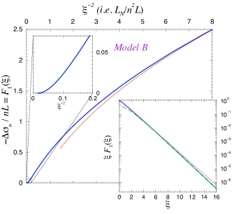
Figure 8: $\Delta\tilde{\sigma}_{n}\propto{}F_{1}(\xi)$ (continuous blue line) as a function of $1/\xi^{2}\propto L_{N}/n^{2}L$. Comparison with the limiting behaviour $F_{1}(\xi\ll 1)\simeq 1.191/\xi-0.877$ (red dotted line). Inset : $\xi\,F_{1}(\xi)$ in semi-log scale. For moderate values of $\xi$, the function is well fitted by $1.21\,{\mbox{\large e}}^{-0.9\xi}$ (magenta dots). Green dashed curve is the asymptotic expression, eq. (51).

We first consider the limit $L_{N}\ll n^{2}L$. Eq. (50) gives $g(\Lambda\gg 1)\simeq\frac{1}{\sqrt{2}}{\mbox{\large e}}^{-\Lambda}\int_{0}^{\infty}\frac{\mathrm{d}{x}}{8x^{3/2}}(1-{\mbox{\large e}}^{-\Lambda{}x})=\frac{1}{4\sqrt{2}}\sqrt{\pi\Lambda}\,{\mbox{\large e}}^{-\Lambda}$, therefore $F_{1}(\xi\gg 1)\simeq\frac{1}{2}|u_{1}|^{-13/8}\sqrt{\pi/\xi}\,{\mbox{\large e}}^{-|u_{1}|^{1/4}\xi}$ and

$$\boxed{\Delta\tilde{\sigma}_{n}(x)\simeq-\frac{L\,n\sqrt{\pi}}{2^{\frac{5}{4}}|u_{1}|^{\frac{13}{8}}}\left(\frac{L_{N}}{n^{2}L}\right)^{\!1/4}\!{\mbox{\large e}}^{-\kappa_{2}n\sqrt{L/L_{N}}}}$$ (51)

$$\hskip 14.22636pt\sim T^{-1/12}{\mbox{\large e}}^{-n\,L^{1/2}T^{1/6}}\hskip 7.11317pt\mbox{for }L\ll L_{N}\ll n^{2}L\>,$$ (52)

where $\kappa_{2}=\sqrt{2}|u_{1}|^{1/4}\simeq 1.421$.

For the lowest temperature $n^{2}L\ll L_{N}$, eq. (49) gives $g(0)=\frac{1}{4\sqrt{\pi}}\Gamma(3/4)^{2}$. Therefore $F_{1}(\xi\ll 1)\simeq{}A_{1}/\xi$ with $A_{1}=\frac{1}{2}\sqrt{2/\pi}\,\Gamma(3/4)^{2}\sum_{m=1}^{\infty}|u_{m}|^{-7/4}\simeq 1.191$ (the sum is $\sum_{m=1}^{\infty}|u_{m}|^{-7/4}\simeq 1.989$)

$$\boxed{\Delta\tilde{\sigma}_{n}(x)\simeq-A_{1}\sqrt{\frac{L_{N}L}{2}}\hskip 14.22636pt\mbox{for }n^{2}L\ll L_{N}}\>.$$ (53)

Comparison between models A & B.– We have seen that for the wire, the MC obtained from the two models are related through $L_{\varphi}\to\sqrt{2}\,L_{N}$ (cf. section IV). It is tempting to look for a similar relation for the connected ring in the limit $L\ll{}L_{N}$.

Let us compare the results for the two models of decoherence. In the limit $n^{2}L\ll{}L_{N}$ the expressions (53) is very close to (38) because in this case, the harmonics involve an integral over time of the function $\langle{\mbox{\large e}}^{\mathrm{i}\Phi}\rangle_{V,\mathcal{C}_{t}}$. Therefore harmonics are insensitive to the details of this function but only to the scale over which it decays. In the other limit $L_{N}\ll{}n^{2}L$, the calculation of the harmonics rather involves the tail of the function $\langle{\mbox{\large e}}^{\mathrm{i}\Phi}\rangle_{V,\mathcal{C}_{t}}$. Eq. (51) presents an exponential decays similar to eq. (38), with a different pre-exponential power law since the decay $\langle{\mbox{\large e}}^{\mathrm{i}\Phi}\rangle_{V,\mathcal{C}_{t}}\propto\sqrt{t/\tau_{N}}{\mbox{\large e}}^{-|u_{1}|t/\tau_{N}}$ is different from the simple exponential decay ${\mbox{\large e}}^{-t/\tau_{\varphi}}$ for model A. The additional $\sqrt{t}$ in model B explains the different pre-exponential terms in eqs. (38) and (51).

Could we map the results of the two models through a simple substitution of phase coherence length, as for the infinite wire ? In the regime $L\ll{}L_{N}\ll{}n^{2}L$ we should compare the exponentials of (38) and (51) what leads to $L_{\varphi}\to{}L_{N}/\sqrt{|u_{1}|}\simeq 0.99L_{N}$, however pre-exponential factors cannot be matched, obviously. In the regime $L_{N}\gg{}n^{2}L$ we rather compare the square roots (38) and (53) and therefore $L_{\varphi}\to{}A_{1}^{2}L_{N}\simeq 1.418L_{N}$. Despite there is no unique simple substitution, we get in both cases $L_{\varphi}\sim{}L_{N}$.

Conductivity vs conductance.– We discuss the relation to the conductance. In the regime $L_{N}\gg{}L$ discussed in this section, we expect

$$\Delta{g}_{n}\sim\frac{L_{N}}{\mathcal{L}^{2}}\Delta\tilde{\sigma}_{n}(x)$$ (54)

for $x\in$ ring, for the same reason as for model A, eq. (44), (the factor $L_{N}$ comes from the fact that the integral (8) is dominated by regions of typical size $L_{N}$ in the arms).

VI The chain of rings

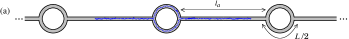
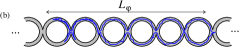
Figure 9: Chains of rings. If we consider the regime $l_{a}\gg{L_{\varphi}}($or $L_{N})\gg{L}$ the rings of figure (a) can be considered as independent. On the other hand, in the regime ${L_{\varphi}}($or $L_{N})\gg{}l_{a},\,{L}$ interferences occur between trajectories encircling several rings ; these latter cannot be anymore considered as independent in this case, as illustrated by the trajectory in the network (b).

Let us consider now a chain of rings separated by arms of lengths $l_{a}$ (figure 9.a). The case where the phase coherence length remains smaller than the arms ($L_{\varphi}\lesssim{}l_{a}$) can be obtained from the results of the previous section since the rings can be considered as independent. The conductance of a chain of such $N_{r}$ rings is given by performing the substitution $\frac{1}{\mathcal{L}^{2}}\to\frac{N_{r}}{[(N_{r}+1)l_{a}+N_{r}l_{c\parallel{}d}]^{2}}$ in the expression of $\Delta{g}_{n}$ for one ring, eqs. (43,44,54).

When arms separating the rings are smaller than the phase coherence length ($l_{a}\lesssim{}L_{\varphi}$), coherent trajectories enclose magnetic fluxes in several rings. In order to study how the MC harmonics are affected by this effect we consider the limit when rings are directly attached to each other (figure 9.b).

VI.1 Model A

Considering the conductance of the symmetric chain of figure 9.b, the weights of the wires involved in eq. (8) are all equal. This justifies a uniform integration of the Cooperon in the chain. In this case we can use the relation between the WL correction and the spectral determinant Pas98 ; PasMon99 ; AkkComDesMonTex00 (appendix D). The spectral determinant of the infinite chain is given in appendix F.2. Averaging the Cooperon in the chain, $\Delta\tilde{\sigma}(\theta)\equiv\int_{\mathrm{chain}}\frac{\mathrm{d}{}x}{\mathrm{Vol}}\Delta\tilde{\sigma}(x,\theta)$, and using (148,169), we finally obtain DouRam86

$$\Delta\tilde{\sigma}(\theta)=-\frac{L_{\varphi}}{2}\left(\coth(L/2L_{\varphi})-\frac{2L_{\varphi}}{L}+\frac{\sinh(L/2L_{\varphi})}{\sqrt{\cosh^{2}(L/2L_{\varphi})-\cos^{2}(\theta/2)}}\right)\>,$$ (55)

where $\theta=4\pi\phi/\phi_{0}$ is the reduced flux per ring. We now study the harmonics $n\neq 0$ :

$$\Delta\tilde{\sigma}_{n}=-\frac{L_{\varphi}}{\sqrt{2}}\,\int_{0}^{2\pi}\frac{\mathrm{d}\theta}{2\pi}\frac{\sinh(L/2L_{\varphi})\,{\mbox{\large e}}^{\mathrm{i}n\theta}}{\sqrt{\cosh(L/L_{\varphi})-\cos(\theta)}}=-L_{\varphi}\,\sinh(L/2L_{\varphi})\oint_{\mathrm{circle}}\frac{\mathrm{d}z}{2\mathrm{i}\pi}\frac{z^{n-1}}{\sqrt{({\mbox{\large e}}^{L/L_{\varphi}}-z)(z-{\mbox{\large e}}^{-L/L_{\varphi}})/z}}\>.$$ (56)

The integration in the complex plane is performed along the unit circle in the clockwise direction. The segment of the real axis $[0,{\mbox{\large e}}^{-L/L_{\varphi}}]$ is a branch cut. The contour of integration is deformed to follow closely this segment. We obtain :

$$\Delta\tilde{\sigma}_{n} =-\frac{L}{2\pi}\,\frac{\sinh(L/2L_{\varphi})}{L/2L_{\varphi}}\,{\mbox{\large e}}^{-(n-1/2)L/L_{\varphi}}\int_{0}^{1}\mathrm{d}u\,\frac{(1-u)^{n-1/2}}{\sqrt{u^{2}+\varepsilon\,u}}$$ (57)

with $\varepsilon={\mbox{\large e}}^{2L/L_{\varphi}}-1$. We recognize the integral representation (C) of the hypergeometric function gragra  $F$ :

$$\boxed{\Delta\tilde{\sigma}_{n}=-\frac{L}{2\pi}\,\frac{\sinh(L/2L_{\varphi})}{L/2L_{\varphi}}\,{\mbox{\large e}}^{-(n+1/2)L/L_{\varphi}}\,B\!\left(\frac{1}{2},n+\frac{1}{2}\right)\,F\!\left(\frac{1}{2},n+\frac{1}{2};n+1;{\mbox{\large e}}^{-2L/L_{\varphi}}\right)}\>,$$ (58)

where $B(x,y)$ is the Euler $\beta$ function.

Weakly coherent limit.– We consider the limit $L_{\varphi}\ll L$. Using $F(\alpha,\beta;\gamma;\xi\to 0)\to 1$, we obtain :

$$\Delta\tilde{\sigma}_{n}\simeq-\frac{(2n-1)!!}{2^{n+1}\,n!}\,L_{\varphi}\,{\mbox{\large e}}^{-nL/L_{\varphi}}\hskip 14.22636pt\mbox{ for }L_{\varphi}\ll L\>,$$ (59)

a result reminiscent of the result of the isolated ring (3), with a different prefactor originating from the probability to cross the vertices of coordination number $4$ (note that $\frac{(2n-1)!!}{2^{n+1}\,n!}=\frac{\Gamma(n+1/2)}{2\sqrt{\pi}\,n!}\simeq\frac{1}{\sqrt{4\pi n}}$ for $n\gg 1$).

Large coherence length.– In the opposite limit limit $L_{\varphi}\gg{L}$. Eq. (141) gives :

$$\Delta\tilde{\sigma}_{n}\simeq-\sqrt{\frac{L_{\varphi}L}{8\pi n}}\,{\mbox{\large e}}^{-nL/L_{\varphi}}\hskip 7.11317pt\mbox{ for }L\ll L_{\varphi}\ll nL\>.$$ (60)

We have recovered an exponential damping of the harmonics, reminiscent of (3,59), but with a different $L_{\varphi}$ dependence of the pre-exponential factor.

On the other hand, for harmonics with $nL\ll{}L_{\varphi}$, the harmonics can be expanded by using eq. (140). Let us introduce $b_{n}=\ln{n}-\psi(n+\frac{1}{2})+\psi(1)$. These coefficients converge to a finite limit at large $n$ : $b_{n}=-$C$-\frac{1}{24n^{2}}+O(\frac{1}{n^{4}})$, where C$=-\psi(1)=0.577215...$ is the Euler constant. Finally we obtain

$$\Delta\tilde{\sigma}_{n}\simeq-\frac{L}{2\pi}\,\left[\ln(2L_{\varphi}/nL)+b_{n}\right]\hskip 7.11317pt\mbox{ for }nL\ll L_{\varphi}\>.$$ (61)

It is useful to remark that the expressions (60) and (61) coincide with the limiting behaviours of the modified Bessel function $K_{0}(z)$ for large $n$ (the proof is given in appendix C) :

$$\Delta\tilde{\sigma}_{n}\simeq-\frac{L}{2\pi}\,K_{0}(nL/L_{\varphi})\hskip 7.11317pt\mbox{ for }L\ll L_{\varphi}\>.$$ (62)

Up to a factor $1/2$ interpreted below, this expression coincides with the MC harmonics for a long hollow cylinder AltAroSpi81 , eq. (102) recalled in section VIII. We compare this approximation with the exact expression (58) on figure 10. We see that the approximation is already good for $n=1$, provided $L_{\varphi}\gtrsim L$. The difference rapidly diminishes as $n$ increases.

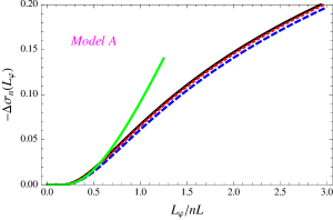
Figure 10: Comparison between exact result (58) for $n=1$ (dashed blue line) and $2$ (dotted red line) and the approximation (62) (black continuous line). The interrupted green curve is (59). Even for small $n$ ($=2$) eq. (62) is a very good approximation of eq. (58).

Logarithmic divergence of the harmonics for $L_{\varphi}\to\infty$.– We see from eq. (61) that the harmonics are weakly dependent on $n$ (for $n\ll{}L_{\varphi}/L$). This logarithmic behaviour reflects the singular behaviour $\Delta\tilde{\sigma}_{\mathrm{osc}}(\theta)\sim 1/\theta$, with a cutoff at $\theta\sim{L/L_{\varphi}}$ : $\Delta\tilde{\sigma}_{n}\sim\int^{1/n}_{L/L_{\varphi}}\frac{\mathrm{d}\theta}{\theta}=\ln(L_{\varphi}/(nL))$. The harmonics are therefore almost independent on $n$ as soon as $n$ is small enough compared to $L_{\varphi}/L$. Note that in practice, this logarithmic divergence of the harmonics is limited : when the phase coherence length reaches the total length of the chain $L_{\varphi}\sim{}N_{r}L$, harmonics reach a finite limit, $\Delta\tilde{\sigma}_{n}\simeq-\frac{L}{2\pi}\ln(N_{r}/n)$, due to the effect of boundaries (external contacts).

Winding probability.– We now extract the probability $\mathcal{P}_{n}(x,x;t)$ from these results. First of all the behaviour (59) is related to

$$\mathcal{P}_{n}(x,x;t)\simeq\frac{(2n-1)!!}{2^{n+1}\,n!}\frac{1}{\sqrt{4\pi t}}\,{\mbox{\large e}}^{-(nL)^{2}/4t}\hskip 14.22636pt\mbox{ for }t\ll L^{2}\>.$$ (63)

We have recovered (12) with an additional dimensionless factor coming from the probability to cross the vertices of coordination number $4$ (this factor can be understood when one writes the trace formula for the heat kernel in the network Rot83 ; AkkComDesMonTex00 ).

The regime $L_{\varphi}\gtrsim{}L$ for the WL correction probes the regime $t\gtrsim{}L^{2}$ for the winding probability. We use the approximation (62) in order to perform the inverse Laplace transform. Using the integral representation of the modified Bessel function gragra , we get :

$$\boxed{\mathcal{P}_{n}(x,x;t)\simeq\frac{L}{8\pi t}\,{\mbox{\large e}}^{-(nL)^{2}/4t}\hskip 14.22636pt\mbox{ for }t\gg L^{2}}\>.$$ (64)

We may check that (60,61) coincide with the limiting behaviours of this probability. It is interesting to point that this probability is similar to the one found for an infinitely long hollow cylinder, apart for a factor $1/2$. This additional factor can be understood from the fact that, starting from a given ring, it is equiprobable to return in one of its two arms.

Let us give a heuristic argument to recover roughly (64), that will be useful for the following. Arriving at a vertex, the diffusive particle equiprobably chooses one of the four arms. Therefore it is equiprobable to wind a ring or not, while diffusing along the chain. This suggests that the winding probability is almost independent on $n$, up to $n\sim\sqrt{t}/L$, the maximum number of rings explored for a time $t$. This rough approximation would be $\mathcal{P}_{n}(x,x;t)\sim\mathcal{N}_{t}\,\theta(\sqrt{t}/L-|n|)$. The normalisation is estimated easily : since diffusion along the chain is one-dimensional, we expect $\sum_{n}\mathcal{P}_{n}(x,x;t)\sim 1/\sqrt{t}$ so that $\mathcal{P}_{n}(x,x;t)\sim{}L/t$ for $|n|\lesssim\sqrt{t}/L$ and $\mathrm{𝟎}$ otherwise. This is a crude estimate of eq. (64).

VI.2 Model B

In order to compute the MC harmonics we first need to construct the function $W$ entering in eq. (15). Following appendix F, we introduce a coordinate $\tilde{x}=(x,f)$ to locate a point in the chain (the continuous variable $x$ measures the distance along the chain while the discrete index $f\in\{u,d\}$ precise the arm, up or down). If $\tilde{x}$ and $\tilde{x}^{\prime}$ do not belong to the same ring we have

$$W(\tilde{x},\tilde{x}^{\prime})=\frac{1}{4}|x-x^{\prime}|=\frac{1}{2}\,W_{\mathrm{wire}}(x,x^{\prime})\>.$$ (65)

Remembering that $W(x,x^{\prime})$ is proportional to the resistance between points $x$ and $x^{\prime}$ this equation has a clear meaning : when two consecutive nodes are linked by two wires instead of one, the resistance is diminished by a factor of $2$. In the limit $t\gg L_{N}^{2}$ the trajectories contributing to

$$\langle{\mbox{\large e}}^{\mathrm{i}\Phi_{V}[\mathcal{C}^{n}_{t}]}\rangle_{V,\mathcal{C}^{n}_{t}}=\left\langle{\mbox{\large e}}^{-\frac{2}{L_{N}^{3}}\int_{0}^{t}\mathrm{d}\tau\,W(x(\tau),x(t-\tau))}\right\rangle_{\mathcal{C}^{n}_{t}}$$ (66)

are trajectories extending over distances $L_{N}\gg{L}$ along the chain. In this case we can neglect the contributions to the integral where the two arguments of $W(\tilde{x},\tilde{x}^{\prime})$ are in the same ring. We have seen that for $nL\lesssim\sqrt{t}$ the measure of the Brownian paths weakly depends on $n$, therefore we expect that $\langle{\mbox{\large e}}^{\mathrm{i}\Phi}\rangle_{V,\mathcal{C}^{n}_{t}}\simeq\langle{\mbox{\large e}}^{\mathrm{i}\Phi}\rangle_{V,\mathcal{C}_{t}}$, where the average of the l.h.s. is realized among Brownian curves of definite winding whereas the average of the r.h.s. is among all Brownian curves. The argument shows that the function describing decoherence corresponds to the result of the infinite wire in which $L_{N}^{3}\to 2L_{N}^{3}$. This factor $2$ stands from the ratio between the resistance of a wire and of a chain of rings of the same length. Finally :

$$\langle{\mbox{\large e}}^{\mathrm{i}\Phi_{V}[\mathcal{C}^{n}_{t}]}\rangle_{V,\mathcal{C}^{n}_{t}}\simeq f_{\mathrm{wire}}(t/2^{2/3}\tau_{N})\>.$$ (67)

We can use (24) in order to compute $\Delta\tilde{\sigma}_{n}\simeq-2\int_{L^{2}}^{\infty}\mathrm{d}{t}\,\frac{L\,{\mbox{\large e}}^{-(nL)^{2}/4t}}{8\pi{t}}\,f_{\mathrm{wire}}(t/2^{2/3}L_{N}^{2})$. The lower cutoff takes into account the fact that expression of $\mathcal{P}_{n}(x,x;t)$ is only valid for $t\gg{L}^{2}$. However, except if $n=0$, the cutoff is not important and can be replaced by $\mathrm{𝟎}$. Using (24) we obtain :

$$\boxed{\Delta\tilde{\sigma}_{n}\simeq-L\,F_{2}\!\left(2^{-1/3}n{L}/{L_{N}}\right)}$$ (68)

where

$$F_{2}(\xi)=\frac{1}{4}\,\sum_{m=1}^{\infty}\frac{1}{|u_{m}|^{3/2}}{\mbox{\large e}}^{-\sqrt{|u_{m}|}\,\xi}\>.$$ (69)

In the limit $L_{N}\ll nL$ the first term of the series dominates :

$$\boxed{\Delta\tilde{\sigma}_{n}\simeq-\frac{L}{4|u_{1}|^{3/2}}\,{\mbox{\large e}}^{-\kappa_{3}n{L}/{L_{N}}}}$$ (70)

$$\hskip 21.33955pt\sim{\mbox{\large e}}^{-nLT^{1/3}}\hskip 14.22636pt\mbox{for }L\ll L_{N}\ll nL\>,$$ (71)

where $\kappa_{3}=2^{-1/3}|u_{1}|^{1/2}\simeq 0.801$.

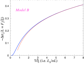
Figure 11: $\Delta\tilde{\sigma}_{n}\propto{}F_{2}(\xi)$ as a function of $1/\xi\propto L_{N}/nL$ (blue continuous line). Comparison with the limiting behaviour (red dotted line) $\frac{1}{2\pi}[\ln(1/\xi)+C_{\mathrm{cyl}}]$ with $C_{\mathrm{cyl}}\simeq 0.51$.

In the opposite limit, for $nL\ll{}L_{N}$ ($\xi\to 0$), we can replace the sum by an integral and use the asymptotic behaviour $u_{m}\simeq-[\frac{3\pi}{2}(m-\frac{3}{4})]^{2/3}$ :

$$F_{2}(\xi)\underset{\xi\to 0}{\simeq}\frac{1}{6\pi}\int_{1}^{\infty}\frac{\mathrm{d}{m}}{m}\,{\mbox{\large e}}^{-\xi[\frac{3\pi}{4}m]^{1/3}}$$ (72)

$$\simeq\frac{1}{6\pi}\int_{1}^{1/\xi^{3}}\frac{\mathrm{d}{m}}{m}+\mathrm{cste}=\frac{1}{2\pi}\,[\ln(1/\xi)+C_{\mathrm{cyl}}]\>.$$ (73)

Finally we find a result similar to the one obtained for exponential relaxation of phase coherence :

$$\boxed{\Delta\tilde{\sigma}_{n}\simeq-\frac{L}{2\pi}\,\left[\ln(L_{N}/nL)+C_{\mathrm{chain}}\right]}\hskip 14.22636pt\mbox{for }nL\ll L_{N}\>.$$ (74)

The constant is estimated numerically : we find $C_{\mathrm{cyl}}\simeq 0.51$, hence $C_{\mathrm{chain}}\simeq 0.74$. This result could also have been more simply obtained by noticing that $f_{\mathrm{wire}}(t/2^{2/3}L_{N}^{2})$ cuts the tail of $\mathcal{P}_{n}(x,x;t)$ on a scale $L_{N}^{2}$ : $\langle\Delta\tilde{\sigma}_{n}\rangle\simeq-2\int_{(nL)^{2}}^{L_{N}^{2}}\mathrm{d}{t}\,\frac{L}{8\pi t}$.

Comparison between models A & B.– As we have done for the infinite wire and the connected ring, we establish some correspondence between the results for the two models when $L_{N}\gg{}L$.

In the regime $L\ll{}L_{N}\ll{}n^{2}L$ the exponentials of (60) and (70) may be matched if $L_{\varphi}\to{}L_{N}/\kappa_{3}\simeq 1.25L_{N}$.

In the regime $L_{N}\gg{}n^{2}L$ the logarithmic behaviours (61) and (74) coincide for $L_{\varphi}\to 1.87\,L_{N}$.

For not too large $n$, the two curves $\Delta\tilde{\sigma}_{n}^{(\mathrm{B})}(L_{N})\approx\Delta\tilde{\sigma}_{n}^{(\mathrm{A})}(L_{\varphi}\simeq 1.87\,L_{N})$ are very close, apart for $L_{N}\ll{}L$ for which there is a qualitative difference between (3) and (27).

From the conductivity to the conductance.– The weights in eq. (8) are all equals and conductance is related to an uniform integration of $\Delta\tilde{\sigma}(x)$ in the chain. The dimensionless conductance is given by $\Delta{g}=\frac{4}{N_{r}L}\Delta\tilde{\sigma}$, where $N_{r}$ is the number of rings of the chain.

VII The square network

The easiest way to realize disorder averaging experimentally is to use networks with a large number of rings, like 2d networks (square DolLicBis86 ; AroSha87 ; Fer04 ; FerAngRowGueBouTexMonMai04 ; SchMalMaiTexMonSamBau07 ; FerRowGueBouTexMon08 , honeycomb PanChaRamGan84 ; PanChaRamGan85 ; AroSha87 , dice Mal06 ; SchMalMaiTexMonSamBau07 ). The “high temperature” regime ($L_{N}\ll L$) is now well understood theoretically and experimentally FerRowGueBouTexMon08 , but low temperature experimental results are still unexplained Mal06 . Therefore understanding the magnetoconductance of large networks when decoherence is dominated by e-e interaction still deserves some clarification. In this section we study the case of an infinite square network of lattice spacing $a$ (figure 1).

VII.1 Model A

The weak localization correction was derived analytically by Douçot & Rammal (DR) for rational fluxes $\theta_{p,q}=2\pi{}p/q$ with $p,\,q\in{\ensmathonze N}$ (reduced flux is defined as $\frac{\theta}{2\pi}=2\phi/\phi_{0}$). They obtained DouRam86

$$\boxed{\Delta\tilde{\sigma}(\theta_{p,q})=-\frac{L_{\varphi}}{2}\left[\coth\frac{a}{L_{\varphi}}-\frac{L_{\varphi}}{a}+\frac{8\sinh\frac{a}{L_{\varphi}}}{\pi q}\,\frac{P^{\prime}_{p,q}(4\cosh\frac{a}{L_{\varphi}})}{P_{p,q}(4\cosh\frac{a}{L_{\varphi}})}\>\mathrm{K}\!\left(\frac{4}{P_{p,q}(4\cosh\frac{a}{L_{\varphi}})}\right)\right]}\>,$$ (75)

where $P_{p,q}(\varepsilon)$ is a polynomial of degree $q$ defined in appendix G.3 where derivation of (75) is recalled. $\mathrm{K}(x)$ is the elliptic integral of the first kind gragra .

Weakly coherent network.– The harmonics are suppressed exponentially as $\Delta\tilde{\sigma}_{n}\propto-L_{\varphi}{\mbox{\large e}}^{-4na/L_{\varphi}}$. Despite there is no close expression of the remaining dimensionless $n$-dependent factor, a systematic expansion of the spectral determinant can be written thanks to the trace formula of Ref. Rot83 (the first terms of this expansion are available in Ref. FerAngRowGueBouTexMonMai04 ).

Large coherence length.– The rest of the section is devoted to the large coherence length regime $L_{\varphi}\gg{}a$.

Continuum limit.– In the limit of small flux, $\theta\ll 1$, and large coherence length, $L_{\varphi}\gg{}a$, the discrete character of the network disappears and one should recover the results for the 2d plane in a uniform magnetic field. Informations can be extracted from the study of this limit.

The zero field WL correction is obtained from eq. (75) with $p=q=1$, using $P_{1,1}(x)=-x$. Using the expansion of the elliptic integral gragra ; footnote9 , we find FerAngRowGueBouTexMonMai04 ; TexMon07c  :

$$\Delta\tilde{\sigma}(0)\simeq-\frac{a}{\pi}\,\left[\ln(4L_{\varphi}/a)+\frac{\pi}{6}\right]\>.$$ (76)

This result is reminiscent of the WL correction of the film (VII.2.1), but here, the cutoff at small scales is naturally provided by the lattice spacing $a$.

The limit of small fluxes is studied in details in appendix G.2. Using that $\theta=4\pi\phi/\phi_{0}=4\pi\mathcal{B}a^{2}/\phi_{0}$, eq. (184) reads

$$\boxed{\Delta\tilde{\sigma}(\theta\ll 1)-\Delta\tilde{\sigma}(0)\simeq\frac{a}{2\pi}\left[\psi\!\left(\frac{1}{2}+\frac{a^{2}}{\theta L_{\varphi}^{2}}\right)-\ln\left(\frac{a^{2}}{\theta L_{\varphi}^{2}}\right)\right]}\>.$$ (77)

This expression gives a quadratic behaviour for small flux footnote14

$$\Delta\tilde{\sigma}(\theta)-\Delta\tilde{\sigma}(0)\simeq\frac{a}{48\pi}\left(\frac{\theta L_{\varphi}^{2}}{a^{2}}\right)^{2}\hskip 14.22636pt\mbox{ for }\theta\ll\frac{a^{2}}{L_{\varphi}^{2}}$$ (78)

and a logarithmic behaviour for intermediate fluxes footnote14

$$\Delta\tilde{\sigma}(\theta)\simeq\frac{a}{2\pi}\left[\ln\theta+C_{\mathrm{sn}}\right]\hskip 14.22636pt\mbox{ for }\frac{a^{2}}{L_{\varphi}^{2}}\ll\theta\ll 1\>,$$ (79)

where $C_{\mathrm{sn}}=-\mathrm{C}-3\ln 2-\frac{\pi}{3}\simeq-3.704$.

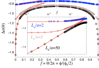
Figure 12: WL correction for $L_{\varphi}/a=2$ (blue diamonds), $L_{\varphi}/a=5$ (brown squares) and $L_{\varphi}/a=50$ (black circles). The red continuous lines correspond to the continuum limit, eqs. (76) and (77).

We now turn to the analysis of the MC harmonics. A first simple remark allows to get the scaling of harmonics with time : the reduced flux $\theta$ is the variable conjugated to the harmonic number $n$, therefore the structure $\Delta\tilde{\sigma}(\theta)=$fct$(a/\sqrt{\theta}L_{\varphi})$ corresponds to $\Delta\tilde{\sigma}_{n}=$fct$(\sqrt{n}a/L_{\varphi})$. We now extract this function. Using the path integral formulation it is straightforward to get the structure

$$\Delta\tilde{\sigma}(\theta)-\Delta\tilde{\sigma}(0) =-2\int_{0}^{\infty}\mathrm{d}t\,\mathcal{P}(x,x;t)$$ (80)

$$\hskip 28.45274pt\times\left(\left\langle{\mbox{\large e}}^{\mathrm{i}\theta\mathcal{N}[\mathcal{C}_{t}]}\right\rangle_{\mathcal{C}_{t}}-1\right){\mbox{\large e}}^{-t/L_{\varphi}^{2}}$$

where $\mathcal{N}[\mathcal{C}_{t}]$ is the winding number of the closed trajectory. At large times the return probability coincides with the one of a plane, $\mathcal{P}(x,x;t)\simeq\frac{a}{4\pi t}$ (appendix F.3) ; it can be obtained from eq. (76) thanks to an inverse Laplace transform. Using gragra $\int_{0}^{\infty}\mathrm{d}{}t\,\big{(}\frac{1}{t}-\frac{\lambda}{\sinh\lambda{}t}\big{)}{\mbox{\large e}}^{-\gamma{}t}=\psi\big{(}\frac{1}{2}+\frac{\gamma}{2\lambda}\big{)}-\ln\big{(}\frac{\gamma}{2\lambda}\big{)}$, we deduce that expression (77) corresponds to $\langle{\mbox{\large e}}^{\mathrm{i}\theta\mathcal{N}[\mathcal{C}_{t}]}\rangle_{\mathcal{C}_{t}}\simeq\frac{\theta\,t}{2a^{2}\sinh(\theta t/2a^{2})}$. A Fourier transform gragra gives the distribution of the winding number, plotted on figure 17,

$$Q_{t}(\mathcal{N})\simeq\frac{\pi a^{2}}{2t\,\cosh^{2}(\pi a^{2}\mathcal{N}/t)}$$ (81)

We have recovered the well-known Levy law for the distribution of the algebraic area $\mathcal{A}=\mathcal{N}a^{2}$ enclosed by a planar Brownian motion KhaWie88 ; Yor89 ; Dup89 ; ComDesOuv90 . For $t\gg a^{2}$ and $n\gg 1$, the return probability conditioned to wind $n$ fluxes is therefore expected to behave as $\mathcal{P}_{n}(x,x;t)\simeq\mathcal{P}(x,x;t)Q_{t}(n)$ :

$$\mathcal{P}_{n}(x,x;t)\simeq\frac{a^{3}}{8\,t^{2}}\,\frac{1}{\cosh^{2}(\pi na^{2}/t)}$$ (82)

A Laplace transform gives the corresponding harmonics

$$\boxed{\Delta\tilde{\sigma}_{n}\simeq-\frac{a}{4\pi n}\,\mathcal{F}_{3}(\pi na^{2}/L_{\varphi}^{2})}$$ (83)

where

$$\mathcal{F}_{3}(\xi)=\int_{0}^{\infty}\mathrm{d}y\,\frac{{\mbox{\large e}}^{-\xi/y}}{\cosh^{2}y}\>.$$ (84)

We extract the following limiting behaviours :

$$\mathcal{F}_{3}(\xi) \underset{\xi\ll 1}{\simeq}1-\xi\,\ln(\xi_{0}/\xi)$$ (85)

$$\underset{\xi\gg 1}{\simeq}\sqrt{4\pi}(2\xi)^{1/4}\,{\mbox{\large e}}^{-\sqrt{8\xi}}\>.$$ (86)

The constant $\xi_{0}$ is estimated numerically : $\xi_{0}\simeq 1.239$. The tail of the distribution corresponds to

$$\boxed{\Delta\tilde{\sigma}_{n}\simeq-\frac{a}{(2n)^{3/4}}\,\sqrt{\frac{a}{\pi L_{\varphi}}}\,{\mbox{\large e}}^{-\sqrt{8\pi n}\>a/L_{\varphi}}}$$ (87)

for $L_{\varphi}\ll\sqrt{n}\,a$. The saturation of the harmonics for $L_{\varphi}\to\infty$ is given by :

$$\boxed{\Delta\tilde{\sigma}_{n}\simeq-\frac{a}{4\pi n}\,\left[1-\frac{\pi na^{2}}{L_{\varphi}^{2}}\ln\left(\frac{L_{\varphi}^{2}\xi_{0}}{\pi na^{2}}\right)\right]}$$ (88)

for $\sqrt{n}\,a\ll L_{\varphi}$.

Harmonics reach a finite limit for $L_{\varphi}\to\infty$.– It is interesting to compare the MC of the chain and the MC of the square network. For the chain, the behaviour of the MC near zero flux $\Delta\tilde{\sigma}^{\mathrm{(chain)}}(\theta)\sim 1/\theta+\mathrm{cste}$, eq. (55), is related to a weak logarithmic divergence of the harmonics $\Delta\tilde{\sigma}^{\mathrm{(chain)}}_{n}\sim\ln(L_{\varphi}/nL)$, eq. (61). For planar networks the WL correction presents a weaker divergence at zero magnetic field $\Delta\tilde{\sigma}(\theta)\sim\ln\theta$. Therefore $\int_{0}^{2\pi}\mathrm{d}\theta\,\Delta\tilde{\sigma}(\theta)<\infty$ and the harmonics reach a finite value in the limit $L_{\varphi}\to\infty$. Let us compute this value. The singular behaviour $\Delta\tilde{\sigma}(\theta)\simeq\mathrm{Cste}+\frac{a}{2\pi}\ln|\theta|$ near zero flux is expected to dominate the harmonics behaviour $\Delta\tilde{\sigma}_{n}\sim\int_{0}\mathrm{d}\theta\,\ln\theta\,\cos(n\theta)$. The typical scale over which $\ln\theta$ varies is $\theta\ln 1/\theta$. If we define $\theta_{c}$ by $\theta_{c}\ln 1/\theta_{c}=1/n$, we see that the integral is dominated by the interval $[0,\theta_{c}]$. We have $\theta_{c}\simeq 1/(n\ln n)$, whence $\Delta\tilde{\sigma}_{n}\sim\int_{0}^{1/(n\ln n)}\mathrm{d}\theta\,\ln\theta\simeq-1/n$. More precisely, we have obtained above : $\Delta\tilde{\sigma}_{n}\simeq-\frac{a}{4\pi n}$ for $n\gg 1$.

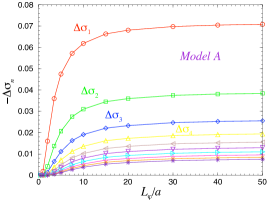
Figure 13: Numerical calculation of ten first MC harmonics $\Delta\tilde{\sigma}_{n}$ for a square network, computed for $L_{\varphi}/a$ between $0.5$ and $50$.

Numerical calculations.– The MC is computed numerically as a function of the reduced flux $\theta$ for rational fluxes $\theta=2\pi p/q$. As recalled in appendix G.3 the computation of the MC is related to the study of the spectrum of a tight binding Hamiltonian on a square lattice submitted to a magnetic field, the so-called Hofstadter problem. For rational flux $\theta=2\pi{}p/q$, this spectrum presents $q$ bands determined by the polynomials $P_{p,q}(\varepsilon)$. For example, band edges correspond to roots of $P_{p,q}(\varepsilon)=\pm 4$. For small $q$ (in practice we choose $\leqslant 8$) the MC is computed by using eq. (75). For large $q$ (large number of Hofstadter bands), we use a more efficient procedure and rather follow Ref. Mon89  : we neglect the dispersion of Hofstadter bands, according to which eq. (G.3) reduces to $\frac{1}{N_{x}N_{y}}\,\mathop{\mathrm{Tr}}\nolimits\left\{\frac{1}{N(\gamma,\theta_{p,q})}\right\}\simeq\>\frac{1}{q}\sum_{r=1}^{q}\frac{1}{4\cosh(\sqrt{\gamma}\,a)+\bar{\varepsilon}_{r}}$, where $\bar{\varepsilon}_{r}$ designates the position of the band. The weak localization correction is represented on figure 12 as a function of the reduced flux $\theta$ for three values of the ratio $L_{\varphi}/a$. As this latter increases, the MC becomes sharper around zero flux, according to the above discussion and the harmonic content becomes richer. The MC is computed in this way for different values of the phase coherence length ranging from $L_{\varphi}/a=0.5$ to $50$. For each curve the first ten harmonics are extracted and plotted as a function of $L_{\varphi}/a$ on figure 13.

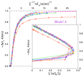
Figure 14: The harmonics represented on Fig. 13 are plotted here as a function of the variable $\sqrt{\xi}=L_{\varphi}/a\sqrt{\pi n}$. The magenta dashed line corresponds to the continuum limit : function $\mathcal{F}_{3}(\xi)$. Inset : Same functions as a function of $\xi\ln(\xi_{0}/\xi)$ with $\xi_{0}\simeq 1.239$.

In order to analyze the numerical results, we use the discussion of the above paragraph on the continuum limit. In the limit $L_{\varphi}\gg a$ we expect the scaling $n_{t}\sim t/a^{2}$. On figure 14, we plot $\frac{4\pi{}n}{a}\Delta\tilde{\sigma}_{n}$ as a function of $1/\sqrt{\xi}=L_{\varphi}/a\sqrt{\pi{}n}$ (note that the scaling $n_{t}\sim t/a^{2}$ is only expected for $L_{\varphi}\gtrsim{a}$ when we reach a “two-dimensional limit” ; for $L_{\varphi}\lesssim{a}$ we rather expect the scaling corresponding to the isolated ring $n_{t}\sim\sqrt{t}/a$).

After rescaling, all curves of figure 13 collapse onto each other as we can see on figure 14 (at least in the domain $L_{\varphi}\gtrsim{a}$). Some significant deviation from expression (83) occurs only for $n=1$. In order to analyze the behaviour for largest $L_{\varphi}$ more precisely, harmonics are re-plotted as funtions of the variable $\xi\ln(\xi_{0}/\xi)$ on the inset of figure 14 : we check the linear behaviour with this variable. Surprisingly, the continuum limit can be considered as a very good approximation already for $n\geqslant 2$.

Remark : Brownian path/random walk.– We have shown that the distribution of the number $n\in{\ensmathonze Z}$ of cells enclosed by a Brownian path in the square lattice is very close from the Levy law describing the distribution of the algebraic area enclosed by a planar Brownian motion (continuum limit) already for $n\geqslant 2$. It is interesting to point out that this remark also holds for the number of cells enclosed by a discrete random walk jumping between the different nodes of the square lattice BelCamBarCla97 ; Des08 .

VII.2 Model B

VII.2.1 The two-dimensional limit

The thin film.– Let us first recall some known results for the plane (or thin film of thickness $b$) AltAroKhm82 ; AltAro85 ; AleAltGer99 . In two dimensions the diffuson presents a logarithmic behaviour. The function $W$ behaves in the same way, with a cutoff at small scales at the thermal length $L_{T}$ footnote7 ; AltAroKhm82 ; AltAro85 ; footnote10  : $W(\vec{r},\vec{r}\,^{\prime})=\frac{1}{2\pi}\ln(||\vec{r}-\vec{r}\,^{\prime}||/L_{T})$ for $||\vec{r}-\vec{r}\,^{\prime}||\gtrsim{}L_{T}$. Therefore the functional governing decoherence behaves as

$$\Gamma[\mathcal{C}_{t}]\,t\equiv\frac{1}{2}\langle\Phi_{V}[\mathcal{C}_{t}]^{2}\rangle_{V}\sim\frac{2e^{2}T}{\sigma_{0}b}\,t\,\frac{1}{2\pi}\ln\frac{\sqrt{Dt}}{L_{T}}\>.$$ (89)

We recognize the sheet resistance footnote11 $R_{\square}=1/(b\sigma_{0})$ of the film of thickness $b$. The phase coherence (Nyquist) time is evaluated from $\Gamma[\mathcal{C}_{t}]\,t\sim 1$. We obtain the temperature dependence AltAroKhm82 ; AltAro85 ; AleAltGer99

$$\frac{1}{\tau_{N}^{\mathrm{film}}}=\frac{R_{\square}}{h/e^{2}}\,T\,\ln\left[\frac{h/e^{2}}{2R_{\square}}\right]\>,$$ (90)

valid for $L_{T}\gg{}b$. This behaviour was observed experimentally for thin metallic film EchThoGouBoz92 and two-dimensional electron gas EshEisKarPal06 . We recall that 2d magnetoconductance is given by Ber84 ; AkkMon07 ; footnote12  :

$$\Delta\sigma^{\mathrm{film}}(\mathcal{B}) =\frac{2e^{2}}{h}\,\frac{1}{2\pi b}$$

$$\times\left[\psi\!\left(\frac{1}{2}+\frac{\tau_{\mathcal{B}}}{\tau_{N}^{\mathrm{film}}}\right)-\ln\left(\frac{\tau_{\mathcal{B}}}{\tau_{e}}\right)\right]+\mbox{cste}$$ (91)

where $\tau_{\mathcal{B}}=\phi_{0}/(8\pi{D}\mathcal{B})$ and $\psi(z)$ is the Digamma function footnote14 (the additional factor $1/2$ in the Digamma function, compared to (77), is explained in appendix G.2). We may simply write $\Delta\sigma\simeq-\frac{2e^{2}}{h}\,\frac{1}{2\pi{}b}\ln[\mathop{\mathrm{min}}\nolimits\left(\tau_{N}^{\mathrm{film}},\tau_{\mathcal{B}}\right)/\tau_{e}]+$cste. The small time cutoff $\tau_{e}$ in eq. (VII.2.1) is introduced by hand to account for the fact that the diffusion approximation only holds for times footnote13  $t\gtrsim\tau_{e}$.

The square network.– For large time scale ($\tau_{\varphi}\sim{}t\gg{a}^{2}$) and small magnetic fields (such that $\phi\ll\phi_{0}$) the result for the network should coincide with the one for a plane. In this case the function $W$ entering the decoherence rate is $W(x,x^{\prime})\simeq\frac{a}{2\pi}\ln(||x-x^{\prime}||/a)$ where $||x-x^{\prime}||$ is the distance between the two points of the network. The logarithmic behaviour is now cut off naturally at the scale $a$. Because the function $W$ presents a smooth logarithmic behaviour, we extract the relevant time scale (phase coherence time) by following the same lines as for the plane. We write

$$\Gamma[\mathcal{C}_{t}]\,t \equiv\frac{1}{2}\langle\Phi_{V}[\mathcal{C}_{t}]^{2}\rangle_{V}$$

$$\sim\frac{2D}{L_{N}^{3}}\,t\,\frac{a}{2\pi}\ln\frac{\sqrt{Dt}}{a}=\frac{2e^{2}T}{\sigma_{0}s}\,t\,\frac{a}{2\pi}\ln\frac{\sqrt{Dt}}{a}$$ (92)

where $s=wb$ is the section of the wires of width $w$ and thickness $b$ (figure 1). From this expression we extract a time scale reminiscent of eq. (90) for the film :

$$\boxed{\frac{1}{\tau^{\mathrm{net}}_{N}}=\frac{R_{\square}^{\mathrm{net}}}{h/e^{2}}\,T\,\ln\left[\frac{L_{T}^{2}}{a^{2}}\frac{h/e^{2}}{2R_{\square}^{\mathrm{net}}}\right]}\>.$$ (93)

This result is valid for $L_{T}\lesssim{}a$. In the opposite limit $L_{T}\gtrsim{}a$, the cutoff in the function $W$ should rather be footnote7 $L_{T}$ therefore $1/\tau^{\mathrm{net}}_{N}=\frac{R_{\square}^{\mathrm{net}}}{h/e^{2}}\,T\,\ln\big{[}\frac{h/e^{2}}{2R_{\square}^{\mathrm{net}}}\big{]}$. However this latter regime seems less relevant from the experimental point of view footnote4 . The sheet resistance of the network is

$$R_{\square}^{\mathrm{net}}=\frac{a}{wb\sigma_{0}}=\frac{a}{s\sigma_{0}}=R_{\square}\frac{a}{w}\>.$$ (94)

This characteristic time is reduced by a factor $w/a$, compared to the Nyquist time (90) obtained for a film of same thickness : $\tau^{\mathrm{net}}_{N}\sim\frac{w}{a}\tau^{\mathrm{film}}_{N}$. We can also introduce a Nyquist length for the network $L_{N}^{\mathrm{net}}=\sqrt{D\tau^{\mathrm{net}}_{N}}$, related to the Nyquist length of the wire $L_{N}$ by footnote15  :

$$\boxed{\frac{1}{L_{N}^{\mathrm{net}}}=\frac{1}{L_{T}}\,\sqrt{\frac{R_{\square}^{\mathrm{net}}}{h/e^{2}}\,\ln\left[\frac{L_{T}^{2}}{a^{2}}\frac{h/e^{2}}{2R_{\square}^{\mathrm{net}}}\right]}=\sqrt{\frac{3\,a}{2\pi L_{N}^{3}}\,\ln(L_{N}/a)}}\>.$$ (95)

We expect that the MC presents the logarithmic behaviour $\Delta\tilde{\sigma}\simeq\frac{a}{2\pi}[\ln\theta+C_{\mathrm{sn}}]$ which is cut off at very low magnetic field : $\Delta\tilde{\sigma}\simeq-\frac{a}{\pi}\ln[\mathop{\mathrm{min}}\nolimits\left(L_{N}^{\mathrm{net}},L_{\mathcal{B}}\right)/a]$, where $L_{\mathcal{B}}=\sqrt{\phi_{0}/(4\pi\mathcal{B})}$ is the 2d cutoff.

VII.2.2 MC Harmonics

In the network, the diffuson behaves logarithmically at large distances $P_{d}(x,x^{\prime})\simeq-\frac{a}{2\pi}\ln(||x-x^{\prime}||/a)$. Therefore we expect that the relaxation of phase coherence is controlled by

$$\frac{1}{2}\langle\Phi_{V}[\mathcal{C}_{t}]^{2}\rangle_{V,\mathcal{C}_{t}}\sim\frac{a}{\pi L_{N}^{3}}\,t\,\ln(\sqrt{t}/a)\to\frac{3a}{2\pi L_{N}^{3}}\,t\,\ln(L_{N}/a)\>.$$ (96)

As for the plane we use the fact that the functional describing decoherence weakly depends on trajectories since $W(x,x^{\prime})\sim\ln||x-x^{\prime}||$. This suggests that the result for model B is given by performing, in the result for model A, the substitution

$$\frac{1}{L_{\varphi}^{2}}\to\frac{3a}{2\pi L_{N}^{3}}\ln(L_{N}/a)\hskip 14.22636pt\mbox{ {\it i.e.} }\hskip 14.22636ptL_{\varphi}\to L_{N}^{\mathrm{net}}\>,$$ (97)

where the Nyquist length for the network is given by (95). Using (87), we get for the tail :

$$\Delta\tilde{\sigma}_{n} \sim\left(L_{N}^{\mathrm{net}}\right)^{-1/2}{\mbox{\large e}}^{-\sqrt{8\pi n}\,a/L_{N}^{\mathrm{net}}}$$ (98)

$$\sim L_{N}^{-3/4}\ln^{1/4}\big{(}\frac{L_{N}}{a}\big{)}\,{\mbox{\large e}}^{-\sqrt{n}\,(\frac{a}{L_{N}})^{3/2}\ln^{1/2}(\frac{L_{N}}{a})}$$

$$\sim(T\ln 1/T)^{1/4}\>{\mbox{\large e}}^{-n^{1/2}a^{3/2}(T\ln 1/T)^{1/2}}\>.$$ (99)

A similar substitution in eq. (88) leads to

$$\Delta\tilde{\sigma}_{n}\sim-\frac{a}{4\pi n}\left[1-\frac{9na^{3}}{2L_{N}^{3}}\ln^{2}(L_{N}/a)\right]$$ (100)

to describe the saturation of the harmonics at large $L_{N}/a$ (small temperature).

We insist that since $\int_{0}\mathrm{d}\theta\,\Delta\sigma(\theta)<\infty$ the harmonics reach a limit for $L_{\varphi}\to\infty$ (or $L_{N}\to\infty$) which is independent on the decoherence mechanism. In other terms the magnetoconductance curve $\Delta\tilde{\sigma}(\theta)$ reaches a limit apart in a very narrow region of width $\delta\theta\sim{}(a/L_{\varphi})^{2}$ around zero flux (figure 12).

VIII The hollow cylinder

We have noticed that a network made of a large number of rings realizes disorder averaging. Another natural way to realize this averaging is to consider a long hollow cylinder of perimeter $L$ (longer than $L_{\varphi}$) submitted to a magnetic field along its axis AltAroSpi81 ; ShaSha81 ; AltAroSpiShaSha82 ; AroSha87 . We study below how the original result of AAS AltAroSpi81 obtained within model A is modified when decoherence is dominated by electron-electron interaction. In this section, it is natural to define the reduced dimensionless conductivity $\tilde{\sigma}$ as $\sigma=\frac{2e^{2}}{h\,b}\tilde{\sigma}$, where $b$ is the thickness of the metallic film.

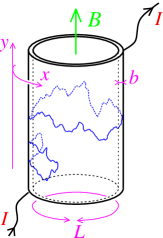
Figure 15: A metallic film is deposited on an insulating wire. This allows to study quantum transport in a long hollow cylinder ShaSha81 . Two diffusive trajectories are represented with winding $n=0$ and $n=1$.

VIII.1 Model A

Let us first recall the well-known result for the weak localization correction computed within model A AltAroSpi81 ; AkkMon07 . We denote by $y\in{\ensmathonze R}$ the coordinate along the axis of the cylinder and $x\in[0,L]$ the coordinate in the perpendicular direction. The WL correction is written as a path integral over Brownian paths $\vec{r}(\tau)=(x(\tau),y(\tau))$ in the cylinder, where $x(\tau)$ describes a Brownian path on the circle and $y(\tau)$ on ${\ensmathonze R}$ (figure 15) :

$$\Delta\tilde{\sigma}_{n}^{\mathrm{AAS}}=-2\,\int_{0}^{\infty}\mathrm{d}{t}\,{\mbox{\large e}}^{-t/\tau_{\varphi}}$$

$$\hskip 42.67912pt\times\int_{\vec{r}(0)=\vec{r}}^{\vec{r}(t)=\vec{r}}\mathcal{D}\vec{r}(\tau)\,\delta_{n,\mathcal{N}[x(\tau)]}\,{\mbox{\large e}}^{-\int_{0}^{t}\mathrm{d}\tau\,\frac{1}{4}\dot{\vec{r}}\,^{2}}$$ (101)

$$=-2\,\int_{0}^{\infty}\mathrm{d}{t}\,{\mbox{\large e}}^{-t/\tau_{\varphi}}\frac{{\mbox{\large e}}^{-(nL)^{2}/4t}}{4\pi t}=-\frac{1}{\pi}\>K_{0}\!\left(\frac{nL}{L_{\varphi}}\right)$$ (102)

where $K_{0}(x)$ is a modified Bessel function. Therefore :

$$\Delta\tilde{\sigma}_{n}^{\mathrm{AAS}} \simeq-\sqrt{\frac{L_{\varphi}}{2\pi nL}}\,{\mbox{\large e}}^{-nL/L_{\varphi}}\hskip 7.11317pt\mbox{ for }L_{\varphi}\ll|nL|$$ (103)

$$\simeq-\frac{1}{\pi}\>\ln\left({L_{\varphi}}/nL\right)\hskip 21.33955pt\mbox{ for }|nL|\ll L_{\varphi}\>.$$ (104)

These results are very similar to the one obtained for the chain of rings (60,61,62). This is due to the similar winding properties, what was already noticed after eq. (64).

VIII.2 Model B : e-e interaction

We have now to consider the path integral

$$\Delta\tilde{\sigma}_{n} =-2\,\int_{0}^{\infty}\mathrm{d}{t}\,$$ (105)

$$\times\int_{\vec{r}(0)=0}^{\vec{r}(t)=0}\mathcal{D}\vec{r}(\tau)\,\delta_{n,\mathcal{N}[x(\tau)]}\,{\mbox{\large e}}^{-\int_{0}^{t}\mathrm{d}\tau\,\big{[}\frac{1}{4}\dot{\vec{r}}\,^{2}+2e^{2}TR_{\square}W(\vec{r}(\tau),0)\big{]}}$$

where we have used translation invariance along the two perpendicular directions in order to deal with a path integral with action local in time, in a similar way as for the ring : eq. (A).

VIII.2.1 The function $W$

The cylinder is translation invariant in the two directions, therefore we may write $W(\vec{r},\vec{r}\,^{\prime})=W(\vec{r}-\vec{r}\,^{\prime},0)$ with $W(\vec{r},0)=P_{d}(\vec{r}_{c},0)-P_{d}(\vec{r},0)$, where $\vec{r}_{c}$ is a short distance cutoff of order $L_{T}$ (we will see that the direction of the vector $\vec{r}_{c}$ plays no role) footnote7 .

In order to avoid the divergent contribution of the zero mode of the Laplace operator, we start by considering the solution of $(\gamma-\Delta)\,P=\delta$ :

$$P(\vec{r},0) =\frac{1}{L}\sum_{n\in{\ensmathonze Z}}\int_{-\infty}^{+\infty}\frac{\mathrm{d}k}{2\pi}\,\frac{{\mbox{\large e}}^{2\mathrm{i}\pi nx/L+\mathrm{i}ky}}{\gamma+(\frac{2\pi n}{L})^{2}+k^{2}}$$ (106)

$$=\frac{1}{2L}\sum_{n\in{\ensmathonze Z}}\frac{1}{\sqrt{\gamma+(\frac{2\pi n}{L})^{2}}}{\mbox{\large e}}^{2\mathrm{i}\pi nx/L-\sqrt{\gamma+(\frac{2\pi n}{L})^{2}}\,|y|}\>.$$ (107)

Next we take the limit $\gamma\to 0$ in

$$W(\vec{r},0) =\lim_{\gamma\to 0}\left[P(\vec{r}_{c},0)-P(\vec{r},0)\right]$$ (108)

$$=\frac{|y|}{2L}+\frac{1}{2\pi}\sum_{n=1}^{\infty}\frac{1}{n}\left(\cos\frac{2\pi nx_{c}}{L}\>{\mbox{\large e}}^{-\frac{2\pi ny_{c}}{L}}\right.$$

$$\hskip 71.13188pt\left.-\cos\frac{2\pi nx}{L}\>{\mbox{\large e}}^{-\frac{2\pi n|y|}{L}}\right)\>.$$ (109)

We finally obtain

$$\boxed{W(\vec{r},0)=\frac{|y|}{2L}+\frac{1}{2\pi}\mathop{\mathrm{Re}}\nolimits\Big{[}\ln\left(\frac{1-{\mbox{\large e}}^{-\frac{2\pi}{L}(\mathrm{i}x+|y|)}}{2\pi L_{T}/L}\right)\Big{]}}$$ (110)

where we used that $||\vec{r}_{c}||=L_{T}\ll{L}$. We can check that this expression reproduces known results in two limits : for $|y|\gg{L}$, we recover the 1d form $W\simeq|y|/(2L)$. For $|y|\ll{L}$ we obtain the 2d result $W\simeq\frac{1}{2\pi}\ln(||\vec{r}||/L_{T})$.

VIII.2.2 Harmonics

The first term of eq. (110) originates from the 1d motion along the cylinder. To this 1d motion, we can associate a 1d Nyquist time similar to the one obtained for the wire, eq. (5),

$$\boxed{\frac{1}{\tau_{N,1d}}=\left(\frac{e^{2}R_{\square}\sqrt{D}T}{L}\right)^{2/3}=\left(\frac{e^{2}\sqrt{D}T}{\sigma_{0}bL}\right)^{2/3}}$$ (111)

that coincides with (5) in which the section is taken as $s=bL$.

We consider first the high temperature limit $L\gg{}L_{N,1d}=\sqrt{D\tau_{N,1d}}=(\frac{\sigma_{0}DbL}{e^{2}T})^{1/3}$. We remark that for the harmonic $n=0$, trajectories very unlikely wind around the cylinder and we can use $W\simeq\frac{1}{2\pi}\ln(||\vec{r}||/L_{T})$ for $y\ll{}L$. Therefore the calculation of the path integral (105) corresponds to the one for the film, $\Delta\sigma_{0}\simeq\Delta\sigma^{\mathrm{film}}$, with the time scale (90).

Next we consider non zero harmonics $n\neq 0$. In this case the trajectories have a small extension along the wire $|y|\lesssim{}L_{N,1d}\ll{}L$ and we can neglect the $|y|$ in the exponential in eq. (110) (see figure 16). Therefore we perform the substitution :

$$W(\vec{r},0)\to\frac{|y|}{2L}+\widetilde{W}(x)$$ (112)

with

$$\widetilde{W}(x)=\frac{1}{2\pi}\ln\frac{|\sin(\pi x/L)|}{\pi L_{T}/L}$$ (113)

This approximation allows us to factorize the path integral as :

$$\Delta\tilde{\sigma}_{n}\simeq-2\,\int_{0}^{\infty}\mathrm{d}{t}\,\int_{x(0)=0}^{x(t)=0}\mathcal{D}x(\tau)\,\delta_{n,\mathcal{N}[x(\tau)]}\,{\mbox{\large e}}^{-\int_{0}^{t}\mathrm{d}\tau\,\big{[}\frac{1}{4}\dot{x}^{2}+2e^{2}TR_{\square}\widetilde{W}(x)\big{]}}\int_{y(0)=0}^{y(t)=0}\mathcal{D}y(\tau)\,{\mbox{\large e}}^{-\int_{0}^{t}\mathrm{d}\tau\,\big{[}\frac{1}{4}\dot{y}^{2}+\frac{|y|}{L_{N,1d}^{3}}\big{]}}\>.$$ (114)

The first path integral runs over trajectories encircling the cylinder. Therefore we can replace $\widetilde{W}(x)$ by its average $\int_{0}^{L}\frac{\mathrm{d}{x}}{L}\widetilde{W}(x)$. This approximation is justified by the fact that $\widetilde{W}$ has only a logarithmic dependence. This simplify the calculation by substituting the functional by a constant :

$$2e^{2}TR_{\square}\int_{0}^{t}\mathrm{d}\tau\,\widetilde{W}(x(\tau))\to\frac{t}{\tau_{N,2d}^{\mathrm{cyl}}}\>,$$ (115)

where we have introduced the time scale

$$\boxed{\frac{1}{\tau_{N,2d}^{\mathrm{cyl}}}=\frac{R_{\square}}{h/e^{2}}\,T\,\ln\left(\frac{L^{2}}{L_{T}^{2}}\right)}\>.$$ (116)

This time is reminiscent of the Nyquist time for the film, eq. (90), but the two times differ by the argument of the logarithm.

The second path integral precisely coincides with the one for a wire : $\frac{1}{\sqrt{4\pi t}}\langle{\mbox{\large e}}^{\mathrm{i}\Phi}\rangle_{V,\mathcal{C}_{t}}$ given by (24). Finally

$$\Delta\tilde{\sigma}_{n} \simeq-2\,\int_{0}^{\infty}\mathrm{d}{t}\,\frac{1}{\sqrt{4\pi{t}}}\,{\mbox{\large e}}^{-\frac{(nL)^{2}}{4t}}{\mbox{\large e}}^{-t/\tau_{N,2d}^{\mathrm{cyl}}}\>$$

$$\times\frac{1}{\sqrt{4\pi t}}\sqrt{\frac{\pi t}{\tau_{N,1d}}}\sum_{m=1}^{\infty}\frac{1}{|u_{m}|}{\mbox{\large e}}^{-|u_{m}|t/\tau_{N,1d}}\>,$$ (117)

which leads to the series (for $n\neq 0$) :

$$\boxed{\Delta\tilde{\sigma}_{n}\simeq-\frac{1}{2\sqrt{\tau_{N,1d}}}\sum_{m=1}^{\infty}\frac{\sqrt{\tau_{m}}}{|u_{m}|}{\mbox{\large e}}^{-nL/\sqrt{\tau_{m}}}}$$ (118)

where the times $\tau_{m}$ are defined as

$$\frac{1}{\tau_{m}}\stackrel{{\scriptstyle\mbox{\tiny def}}}{{=}}\frac{|u_{m}|}{\tau_{N,1d}}+\frac{1}{\tau_{N,2d}^{\mathrm{cyl}}}\>,$$ (119)

(we recall that $u_{m}$’s are zeros of Airy function Ai^′).

This expression assumes that $L\gg{}L_{N,1d}$. We show that (118) it also valid for the other regime $L\ll{}L_{N,1d}$ : in this case the path integral runs over trajectories such that $|y|\gg{}L$ (see figure 16), therefore, in (110), the exponential damping suppresses the $x$ and $y$ dependence in the logarithmic of $W$ what leads to the same conclusion for the two regimes since $W\to\frac{|y|}{2L}+\frac{1}{2\pi}\ln(L/2\pi{}L_{T})$.

In order to analyze the two limiting cases into more details it is convenient to relate the two times as :

$$\frac{\tau_{N,1d}}{\tau_{N,2d}^{\mathrm{cyl}}}=\frac{1}{\pi}\,\left(\frac{L}{L_{N,1d}}\right)\,\ln\left(\frac{L}{L_{T}}\right)\>.$$ (120)

Since the two lengths ${L}_{N,2d}^{\mathrm{cyl}}$ and $L_{N,1d}$ are related, we just have to consider two different regimes. As it is clear from eq. (119), the harmonics are always controlled by the smallest scale among ${L}_{N,2d}^{\mathrm{cyl}}$ and $L_{N,1d}$.

$\bullet$ High temperature $L_{N,1d}\ll{}L$ (then ${L}_{N,2d}^{\mathrm{cyl}}\ll{}L_{N,1d}$).– The WL correction is dominated by non winding trajectories in this case

$$\Delta\tilde{\sigma}\simeq\Delta\tilde{\sigma}_{0}\simeq-\frac{1}{2\pi}\,\ln\left(\frac{\tau_{N}^{\mathrm{film}}}{\tau_{e}}\right)+\mbox{cste}$$ (121)

involves the 2d Nyquist time (90). Considering the oscillating part of the MC, only the first term of the series dominates. The harmonics are governed by the smallest length among ${L}_{N,2d}^{\mathrm{cyl}}$ and $L_{N,1d}$ :

$$\boxed{\Delta\tilde{\sigma}_{n}\simeq-\frac{{L}_{N,2d}^{\mathrm{cyl}}}{2|u_{1}|\,L_{N,1d}}{\mbox{\large e}}^{-nL/L_{N,2d}^{\mathrm{cyl}}}}\sim{\mbox{\large e}}^{-n\,L\,(T\ln T)^{1/2}}$$ (122)

for $L_{N,1d}\ll L$. Note that this result is reminiscent of the result (27) for a ring $\Delta\tilde{\sigma}_{n}^{\mathrm{ring}}\sim{\mbox{\large e}}^{-nL^{3/2}T^{1/2}}$ : up to some logarithmic correction it presents a similar $T^{1/2}$ in the exponential for the similar reason (related to potential fluctuations seen by winding trajectories). However the $L$ dependence differs from the one of the ring.

$\bullet$ Low temperature $L\ll{}L_{N,1d}$ (then $L_{N,1d}\ll{L}_{N,2d}^{\mathrm{cyl}}$).– The harmonics involve $L_{N,1d}$, the smallest length among ${L}_{N,2d}^{\mathrm{cyl}}$ and $L_{N,1d}$. Eq. (118) coincides with the one obtained for the chain of rings (68) :

$$\Delta\tilde{\sigma}_{n}\simeq-2\,F_{2}(nL/L_{N,1d})\>.$$ (123)

For intermediate coherence length, $L\ll L_{N,1d}\ll nL$, eq. (118) gives

$$\boxed{\Delta\tilde{\sigma}_{n}\simeq-\frac{1}{|u_{1}|^{3/2}}{\mbox{\large e}}^{-|u_{1}|^{1/2}nL/L_{N,1d}}}\sim{\mbox{\large e}}^{-nLT^{1/3}}\>.$$ (124)

For largest phase coherence length $nL\ll L_{N,1d}$, we may use the form derived in section VI

$$\boxed{\Delta\tilde{\sigma}_{n}\simeq-\frac{1}{\pi}\left[\ln\left(\frac{L_{N,1d}}{nL}\right)+C_{\mathrm{cyl}}\right]}$$ (125)

where the constant, $C_{\mathrm{cyl}}\simeq 0.51$, was introduced in section VI.

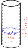
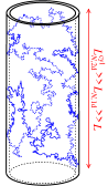
Figure 16: Trajectories contributing to first harmonic for “high temperature” (left) and “low temperature” (right).

Discussion.– It is worth emphasizing the similarity between the results for the cylinder and for the networks.

In section IV we have seen that the MC harmonics of a weakly coherent ring probe two length scales $L_{N}\propto{T}^{-1/3}$ or $L_{c}\propto{T}^{-1/2}$. For the lowest temperatures the surrounding network matters and another length scale emerges : the MC of the square network involves a unique time scale $1/\tau_{N}^{\mathrm{net}}\sim{T}\ln{1/T}$, eq. (95), reminiscent of the 2d Nyquist time (90).

For a cylinder the MC also probes several time scales. At high temperature the zero harmonic related to non-winding trajectories probes the 2d Nyquist time $\frac{1}{\tau_{N}^{\mathrm{film}}}=\frac{R_{\square}}{h/e^{2}}\,T\,\ln[{h/e^{2}}{2R_{\square}}]$ whereas the nonzero harmonics probe the time $\frac{1}{\tau_{N,2d}^{\mathrm{cyl}}}=\frac{R_{\square}}{h/e^{2}}\,T\,\ln[{L^{2}}/{L_{T}^{2}}]$. The main dependence of the corresponding length ${L}_{N,2d}^{\mathrm{cyl}}\propto{}T^{-1/2}$ has the same origin as for a single ring and reflects that winding trajectories feel fluctuations of the potential over length scale given by the perimeter (figure 16, left). For lower temperature, trajectories diffuse along the cylinder over length scale much larger than the perimeter and the WL correction is controlled by a unique length $L_{N,1d}$, corresponding to the usual 1d Nyquist time $\tau_{N,1d}\propto{T}^{-2/3}$.

IX Conclusion

We have studied the weak localization correction in metallic networks and in a hollow cylinder. This study relies on a detailed analysis of the winding properties of closed Brownian trajectories in these systems. We now summarize our results.

We first recall the behaviour of the probability to return to the starting point after a time $t$ for trajectories conditioned to wind $n$ rings. In the short time limit $t\ll{}L^{2}$, we have $\mathcal{P}_{n}(x,x;t)\simeq{}p_{n}\frac{1}{\sqrt{4\pi t}}{\mbox{\large e}}^{-(nL)^{2}/4t}$ where $p_{n}$ depends on the network : $p_{n}=1$ for the isolated ring, $p_{n}=\big{(}\frac{2}{3}\big{)}^{nN_{a}}$ for the ring connected to $N_{a}$ long wires and $p_{n}=\frac{(2n-1)!!}{2^{n+1}n!}$ in the chain of rings. For the square network, there is no close expression but a systematic expansion may be found in Ref. FerAngRowGueBouTexMonMai04 with the trace formula of Ref. Rot83 .

Network	$\mathcal{P}(x,x;t)$	$Q_{t}(n)$	$q(x)$
	$\frac{1}{N_{a}\sqrt{\pi t}}$	$\frac{\sqrt{N_{a}L}}{(4\pi t)^{1/4}}\,q\big{(}\frac{n\sqrt{N_{a}L}}{(4\pi t)^{1/4}}\big{)}$	$\frac{\pi^{3/4}}{\sqrt{2}}\Psi((4\pi)^{1/4}x)$
	$\frac{1}{4\sqrt{\pi t}}$	$\frac{L}{\sqrt{2t}}\,q\big{(}\frac{nL}{\sqrt{2t}}\big{)}$	$\frac{1}{\sqrt{2\pi}}{\mbox{\large e}}^{-\frac{1}{2}x^{2}}$
	$\frac{a}{4\pi t}$	$\frac{2\sqrt{3}a^{2}}{t}\,q\big{(}\frac{n2\sqrt{3}a^{2}}{t}\big{)}$	$\frac{\pi}{4\sqrt{3}}\frac{1}{\cosh^{2}(\frac{\pi x}{2\sqrt{3}})}$

Table 1: Return probability and distribution $Q_{t}(n)=\frac{\mathcal{P}_{n}(x,x;t)}{\mathcal{P}(x,x;t)}$ of the winding number in the large time limit $t\gg{}L^{2}$. The function $\Psi(\xi)$ is defined in eq. (41)

At large times $t\gg{}L^{2}$ the typical winding number scales as $n_{t}\sim{}(t/L^{2})^{\alpha}$, where $\alpha$ is a network dependent exponent. Introducing the return probability $\mathcal{P}(x,x;t)=\sum_{n}\mathcal{P}_{n}(x,x;t)$, we may write the winding probability as

$$\mathcal{P}_{n}(x,x;t)\simeq\frac{\mathcal{P}(x,x;t)}{c_{2}\,(t/L^{2})^{\alpha}}\>q\!\left(\frac{n}{c_{2}\,(t/L^{2})^{\alpha}}\right)\>,$$ (126)

where $\int\mathrm{d}x\,q(x)=1$. The dimensionless number $c_{2}$ ensures that $\int\mathrm{d}x\,x^{2}\,q(x)=1$. Since $\mathcal{P}(x,x;t)\sim{}t^{-d/2}$ where $d$ is the effective dimensionality of the network, we may also write

$$\mathcal{P}_{n}(x,x;t)\sim\frac{1}{t^{\alpha+d/2}}\,q\!\left(\frac{n}{t^{\alpha}}\right)$$ (127)

($L$ may be re-introduced by dimensional analysis). The function $q(x)$ is given for the various networks in the table 1, and represented on figure 17. Surprinsingly the functions for the connected ring and the plane are very close ; they only differ in the wings when functions are exponentially small.

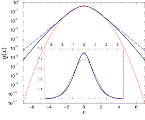
Figure 17: Function $q(x)$ for the connected ring (black continuous line), the chain of rings (red dotted line) and square network (blue dashed line) in semilog scale. Inset : Same functions in linear scale.

We have analyzed in details the harmonics of the magnetoconductance oscillations obtained when decoherence is described by a simple exponential relaxation (model A). In the limit of large coherence length compared to the perimeter of the rings, the scaling of the harmonics can be easily understood from the Laplace transform $\Delta\tilde{\sigma}_{n}\sim\int_{0}^{\infty}\mathrm{d}{}t\,\mathcal{P}_{n}(x,x;t)\,{\mbox{\large e}}^{-t/L_{\varphi}^{2}}$. We see that the time scale coincides with $t\sim{}L_{\varphi}^{2}$. We deduce from (127) that harmonics are of the form

$$\Delta\tilde{\sigma}_{n}\sim\frac{1}{L_{\varphi}^{d-2+2\alpha}}\>\Phi\!\left(\frac{n}{L_{\varphi}^{2\alpha}}\right)\>,$$ (128)

where $\Phi(x)$ is a dimensionless network dependent function (the perimeter $L$ is easily reintroduced by reminding that $\Delta\tilde{\sigma}$ has dimension of a length). We may then summarize for each geometry :

• For the isolated ring ($d=0$, $\alpha=1/2$), the form of the harmonics $\Delta\tilde{\sigma}_{n}\sim{}L_{\varphi}\Phi_{\mathrm{i.r}}(nL/L_{\varphi})$ is related to the scaling $n_{t}\sim t^{1/2}$.

• For the connected ring ($d=1$, $\alpha=1/4$) : $\Delta\tilde{\sigma}_{n}\sim\sqrt{L_{\varphi}L}\,\Phi_{\mathrm{c.r}}(n\sqrt{L/L_{\varphi}})$ can be understood from $n_{t}\sim t^{1/4}$.

• For the chain of rings ($d=1$, $\alpha=1/2$) : $\Delta\tilde{\sigma}_{n}\sim\Phi_{\mathrm{chain}}(nL/L_{\varphi})$ reflects $n_{t}\sim t^{1/2}$.

• For the square network ($d=2$, $\alpha=1$) $\Delta\tilde{\sigma}_{n}\sim\frac{L}{n}\,\tilde{\Phi}_{\mathrm{s.n}}(nL^{2}/L_{\varphi}^{2})$ originates from $n_{t}\sim t$ (here the harmonics were not written exactly under the form (128), but in terms of the function $\tilde{\Phi}(x)=x\Phi(x)$ in order to emphasize that harmonics reach a finite value for $L_{\varphi}\to\infty$).

The precise behaviours for the harmonics $\Delta{}g_{n}$ are summarized in table 2 (we recall that $\Delta{}g_{n}\sim\Delta\sigma_{n}$ apart for the connected ring for which $\Delta{}g_{n}\sim\frac{L_{\varphi}}{l_{a}}\Delta\sigma_{n}$ where $l_{a}$ is the length of the connecting wires).

	Model A (exp. relax.)		Model B (e-e inter.)
		Regime $L_{\varphi}\ll L$
	$L_{\varphi}\,{\mbox{\large e}}^{-nL/L_{\varphi}}$		$L_{N}\,{\mbox{\large e}}^{-\kappa_{1}n(L/L_{N})^{3/2}}$	for $L_{N}\ll L$
	$L_{\varphi}^{1/2}{\mbox{\large e}}^{-nL/L_{\varphi}}$		$\frac{L_{N,2d}^{\mathrm{cyl}}}{L_{N,1d}}{\mbox{\large e}}^{-nL/L_{N,2d}^{\mathrm{cyl}}}$	for $L_{N,2d}^{\mathrm{cyl}}\ll L_{N,1d}\ll L$
		Regime $L_{\varphi}\gg L$
	$L_{\varphi}^{3/2}$	for $n^{2}\ll L_{\varphi}/L$	$L_{N}^{3/2}$	for $n^{2}\ll L_{N}/L$
	$L_{\varphi}^{3/2}{\mbox{\large e}}^{-n\sqrt{2L/L_{\varphi}}}$	for $n^{2}\gg L_{\varphi}/L$	$L_{N}^{5/4}{\mbox{\large e}}^{-\kappa_{2}n\sqrt{L/L_{N}}}$	for $n^{2}\gg L_{N}/L$
	$\ln(L_{\varphi}/nL)$	for $n\ll L_{\varphi}/L$	$\ln(L_{N}/nL)$	for $n\ll L_{N}/L$
	$L_{\varphi}^{1/2}{\mbox{\large e}}^{-nL/L_{\varphi}}$	for $n\gg L_{\varphi}/L$	${\mbox{\large e}}^{-\kappa_{3}nL/L_{N}}$	for $n\gg L_{N}/L$
	$\frac{1}{n}\,\big{[}1-\frac{\pi nL^{2}}{16L_{\varphi}^{2}}\ln(\frac{L_{\varphi}^{2}}{nL^{2}})\big{]}$	for $\sqrt{n}\ll L_{\varphi}/L$	idem for	$L_{\varphi}\to L_{N}^{\mathrm{net}}$
	$L_{\varphi}^{-1/2}{\mbox{\large e}}^{-\sqrt{\frac{\pi}{2}n}\,L/L_{\varphi}}$	for $\sqrt{n}\gg L_{\varphi}/L$	idem for	$L_{\varphi}\to L_{N}^{\mathrm{net}}$
	$\ln(L_{\varphi}/nL)$	for $n\ll L_{\varphi}/L$	$\ln(L_{N,1d}/nL)$	for $n\ll L_{N,1d}/L$
	$L_{\varphi}^{1/2}{\mbox{\large e}}^{-nL/L_{\varphi}}$	for $n\gg L_{\varphi}/L$	${\mbox{\large e}}^{-\kappa_{4}nL/L_{N,1d}}$	for $n\gg L_{N,1d}/L$

Table 2: Harmonics of MC $\Delta{g}_{n}/g$ for different networks. In the high temperature regime $L_{\varphi}\ll L$, winding trajectories cannot explore more than a single ring and harmonics do not depend on the network. Dimensionless constants are $\kappa_{1}=\pi^{2}/8\simeq 1.234$, $\kappa_{2}=\sqrt{2}|u_{1}|^{1/4}\simeq 1.421$, $\kappa_{3}=2^{-1/3}|u_{1}|^{1/2}\simeq 0.801$ and $\kappa_{4}=|u_{1}|^{1/2}\simeq 1.009$. The various Nyquist lengths are $L_{N}\sim{}T^{-1/3}$, $L_{N}^{\mathrm{net}}\sim(T\ln 1/T)^{-1/2}$ and ${L}_{N,2d}^{\mathrm{cyl}}\sim(T\ln{T})^{-1/2}$.

For each situation we have also discussed the effect of decoherence due to electron-electron interaction (model B), the dominant phase breaking mechanism at low temperature. As recalled at the begining of the paper, this mechanism requires a refined description : the simple exponential decay of phase coherence is replaced by a functional of the trajectories, eqs. (15,18). In networks of quasi-1d wires the decoherence due to e-e interaction is controlled by the Nyquist length $L_{N}\propto{T}^{-1/3}$.

In the “high temperature” limit $L_{N}\ll{}L$ the fact that trajectories with finite winding number and trajectories with winding $n=0$ do probe different length scales is responsible for the emergence of two length scales $L_{N}\propto{T}^{-1/3}$ and $L_{c}\propto{T}^{-1/2}$ (or $L_{N}^{\mathrm{film}}\propto{T}^{-1/2}$ and $L_{N,2d}^{\mathrm{cyl}}\propto(T\ln{}T)^{-1/2}$ for the cylinder). The models A & B give different dependences in the phase coherence length : $\Delta\tilde{\sigma}^{(A)}\sim-L_{\varphi}{\mbox{\large e}}^{-nL/L_{\varphi}}$ and $\Delta\tilde{\sigma}^{(B)}\sim-L_{N}{\mbox{\large e}}^{-n(L/L_{N})^{3/2}}$ The exponential decay of harmonics is almost independent on the network.

In the “low temperature” limit $L_{N}\gg{}L$, all trajectories probe the same typical scale, irrespectively of the winding. However this length scale depends on the geometry : $L_{N}\propto{}T^{-1/3}$ for the chains of rings and the hollow cylinder, and $L_{N}^{\mathrm{net}}=(\frac{2\pi{}L_{N}^{3}}{3a})^{1/2}\ln^{-1/2}(L_{N}/a)\sim(T\ln 1/T)^{-1/2}$ for the square network. As a function of the phase coherence length, models A & B predict harmonics of similar form strongly network dependent. We have compared harmonics as a function of the phase coherence length for the different networks on figure 18 (for model A).

All results are summarized in table 2. We have plotted the WL correction to conductances for the three different networks on figure 18.

An experimental verification of these predictions would be interesting and would confirm our understanding of decoherence due to electron-electron interaction in complex geometries. In particular an interesting and clear experimental test would be to compare the MC harmonics for the chain of rings for independent rings and coherent rings (networks of figure 9) in the “low temperature” limit $L_{N}\gg L$. The experimental analysis of the MC harmonics for the square network in this limit seems more difficult due to the fact that harmonics reach a value independent on the phase breaking mechanism. Therefore, contrarily to the chains of rings, the MC harmonics for the square network are less sensitive to the model of decoherence for large phase coherence length.

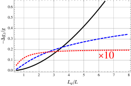
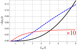
Figure 18: Comparison between harmonics $\Delta{}g_{n}/g$ for different networks in the low temperature regime $L_{\varphi}\gtrsim L$ with $n=1$ and $n=5$. For the connected ring (continuous black line) we choose $l_{a}/L=10$. The blue dashed line corresponds to the chain of rings. The result for the square network (dotted red line) has been multiplied by a factor $10$ for visibility.

Appendix A A useful property of winding Brownian trajectories

The difficulty for computing the path integral (III.2) lies in the time nonlocality of the action. In this appendix we show how it is possible to get rid of time nonlocality in certain cases, as explained in Refs. ComDesTex05 ; TexMon05b . For that purpose we demonstrate the identity

$$\int_{x(0)=x}^{x(t)=x}\mathcal{D}x\,\delta_{n,\mathcal{N}[x]}\,{\mbox{\large e}}^{-\frac{1}{2}\int_{0}^{t}\mathrm{d}\tau\,\dot{x}^{2}-\int_{0}^{t}\mathrm{d}\tau\,V(x(\tau)-x(t-\tau))}$$

$$=\int_{x(0)=0}^{x(t)=0}\mathcal{D}x\,\delta_{n,\mathcal{N}[x]}\,{\mbox{\large e}}^{-\frac{1}{2}\int_{0}^{t}\mathrm{d}\tau\,\dot{x}^{2}-\int_{0}^{t}\mathrm{d}\tau\,V(x(\tau))}$$ (129)

where $x(\tau)$ is a Brownian path on the circle (here identified with the interval $[0,1]$). The identity is valid for any symmetric and periodic function : $V(-x)=V(x)$ and $V(x+n)=V(x)$ for $n\in{\ensmathonze Z}$.

Demonstration for $n=0$ was given in Ref. TexMon05b ; ComDesTex05 , where we pointed that, for a Brownian bridge on ${\ensmathonze R}$ $(x(\tau),\,0\leqslant\tau\leqslant{t}\,|\,x(0)=x(t)=0)$, we have the following equality in law footnote16  :

$$x(\tau)-x(t-\tau)\stackrel{{\scriptstyle\mbox{\tiny(law)}}}{{=}}x(2\tau)\hskip 14.22636pt\mbox{for }0\leqslant\tau\leqslant t/2\>.$$ (130)

The proof lies on the fact that we can relate the bridge to a free Brownian motion (Wiener process) $(W(\tau),\,0\leqslant\tau\leqslant{t},\,W(0)=0)$ : $x(\tau)\stackrel{{\scriptstyle\mbox{\tiny(law)}}}{{=}}W(\tau)-\frac{\tau}{t}W(t)$.

Here we generalize this relation when $x(\tau)$ lives on the circle $[0,1]$ and when we constraint the winding number. Let us unfold the ring in order to work on ${\ensmathonze R}$. A close path winding $n$ times around the ring is related to the following path living on the real axis : $(x_{n}(\tau),\,0\leqslant\tau\leqslant{t}\,|\,\,x_{n}(0)=0\,;\,x_{n}(t)=n)$ that can be writen as

$$x_{n}(\tau)\stackrel{{\scriptstyle\mbox{\tiny(law)}}}{{=}}W(\tau)+\frac{\tau}{t}(n-W(t))\stackrel{{\scriptstyle\mbox{\tiny(law)}}}{{=}}x_{0}(\tau)+n\frac{\tau}{t}$$ (131)

$x_{0}(\tau)$ is the Brownian bridge. It is now easy to show that footnote17

$$x_{n}(\tau)-x_{n}(t-\tau)\stackrel{{\scriptstyle\mbox{\tiny(law)}}}{{=}}x_{n}(2\tau)-n\hskip 14.22636pt\mbox{for }0\leqslant\tau\leqslant t/2\>.$$ (132)

Since $x_{n}(\tau)-x_{n}(t-\tau)$ is argument of the periodic function, the integer shift can be forgotten. The symmetry $V(x)=V(-x)$ ensures the equality of contributions of intervals $\int_{0}^{t/2}$ and $\int_{t/2}^{t}$. It follows that

$$\boxed{\int_{0}^{t}\mathrm{d}\tau\,V(x_{n}(\tau)-x_{n}(t-\tau))\stackrel{{\scriptstyle\mbox{\tiny(law)}}}{{=}}\int_{0}^{t}\mathrm{d}\tau\,V(x_{n}(\tau))}$$ (133)

which demonstrates eq. (A).

Infinite wire : Using (A), we see that the path integral (20) involves an action local in time

$$P_{c}(x,x) \equiv-\frac{1}{2}\Delta\tilde{\sigma}(x)=\int_{0}^{\infty}\mathrm{d}{t}\,{\mbox{\large e}}^{-\gamma t}$$

$$\times\int_{x(0)=0}^{x(t)=0}\mathcal{D}x(\tau)\,{\mbox{\large e}}^{-\int_{0}^{t}\mathrm{d}\tau\,\big{[}\frac{1}{4}\dot{x}^{2}+\frac{1}{L_{N}^{3}}\,|x(\tau)|\big{]}}\>,$$ (134)

that can now be computed. We obtain $P_{c}(0,0)=-L_{N}\,\frac{\mathrm{Ai}(\gamma L_{N}^{2})}{2\,\mathrm{Ai}^{\prime}(\gamma L_{N}^{2})}$ derived in Ref. AltAroKhm82 (numerical factors are incorrect in this reference).

Isolated ring : The function $W(x,x^{\prime})$ is given by eq. (158). The path integral (III.2) can be rewritten as

$$\int_{0}^{\infty}\mathrm{d}{t}\,{\mbox{\large e}}^{-\gamma t}\int_{x(0)=0}^{x(t)=0}\mathcal{D}x\,\delta_{n,\mathcal{N}[x]}\,{\mbox{\large e}}^{-\int_{0}^{t}\mathrm{d}\tau\,\big{[}\frac{\dot{x}^{2}}{4}+\frac{|x|}{L_{N}^{3}}\,\big{(}1-\frac{|x|}{L}\big{)}\big{]}}$$ (135)

that can be expressed in terms of Hermite functions TexMon05b .

Appendix B The function $\Psi(\xi)$

We analyze several properties of the function (41), that we rewrite

$$\Psi(\xi)=\frac{4}{\pi}\Lambda^{3/4}\mathop{\mathrm{Re}}\nolimits\left[{\mbox{\large e}}^{-\mathrm{i}\frac{\pi}{4}}\int_{{\ensmathonze R}^{+}}\mathrm{d}{z}\,z^{2}\,{\mbox{\large e}}^{-\Lambda\,\varphi(z)}\right]\>,$$ (136)

where $\varphi(z)=z^{4}+4z{\mbox{\large e}}^{-\mathrm{i}\pi/4}$ and $\Lambda=(\xi/4)^{4/3}$. The value of the function at the origin is $\Psi(0)=\frac{\Gamma(3/4)}{\pi\sqrt{2}}$.

The asymptotic behaviour for $\xi\gg 1$ may be studied by the steepest descent method. $\varphi^{\prime}(z)=0$ has three solutions $z_{n}={\mbox{\large e}}^{\mathrm{i}\pi/4+2\mathrm{i}{}n\pi/3}$, with $n=0,\,1,\,2$ (figure 19). An appropriate contour deformation in the complex plane of the variable $z$ must remain in the region where $\mathop{\mathrm{Re}}\nolimits[\varphi(z)]>0$. This domain can be easily determined by performing a rotation $z=w{\mbox{\large e}}^{\mathrm{i}\pi/4}$ : writing $w=u+\mathrm{i}{}v$ we have $\mathop{\mathrm{Re}}\nolimits[\varphi(z)]=-u^{4}+6u^{2}v^{2}-v^{4}+4u$ that vanishes for $v=\pm\sqrt{3u^{2}\pm 2\sqrt{2u^{4}+u}}$. The domain where $\mathop{\mathrm{Re}}\nolimits[\varphi(z)]>0$ is represented on figure 19. This shows that the contour can only visit $z_{0}={\mbox{\large e}}^{\mathrm{i}\pi/4}$. The integration over ${\ensmathonze R}^{+}$ is replaced by integration over the segment $\Delta$ from the origin to $z_{0}$ and the contour $\mathcal{C}$ issuing from $z_{0}$ and going to infinity (figure 19). Noticing that $\int_{\Delta}\mathrm{d}{z}\,z^{2}\,{\mbox{\large e}}^{-\Lambda\,\varphi(z)}$ is purely imaginary, we are left with the contribution of the contour $\mathcal{C}$ only. We now use the steepest descent method $\Psi(\xi)=\frac{4}{\pi}\Lambda^{3/4}\mathop{\mathrm{Re}}\nolimits[{\mbox{\large e}}^{-\mathrm{i}\frac{\pi}{4}}\int_{\mathcal{C}}\mathrm{d}{z}\,z^{2}\,{\mbox{\large e}}^{-\Lambda\,\varphi(z)}]\simeq\frac{4}{\pi}\Lambda^{3/4}\mathop{\mathrm{Re}}\nolimits[{\mbox{\large e}}^{-\mathrm{i}\frac{\pi}{4}}\frac{1}{2}\sqrt{\frac{2\pi}{\Lambda\varphi^{\prime\prime}(z_{0})}}{\mbox{\large e}}^{-\Lambda\,\varphi(z_{0})}]$, where the $1/2$ is due to the fact that the contour issues from the stationary point, hence

$$\Psi(\xi\gg 1)\simeq\frac{2}{\sqrt{6\pi}}(\xi/4)^{1/3}{\mbox{\large e}}^{-3(\xi/4)^{4/3}}$$ (137)

(note that a factor $1/2$ is missing in Ref. TexMon05 ).

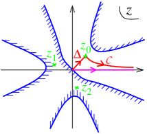
Figure 19: Appropriate contour deformation in order to estimate (136). The dashed area corresponds to the region where $\mathop{\mathrm{Re}}\nolimits[\varphi(z)]<0$.

Finally the relation to the function $q(x)$ introduced in the conclusion requires the two integrals $\int_{0}^{\infty}\mathrm{d}\xi\,\Psi(\xi)=1/\sqrt{\pi}$ and $\int_{0}^{\infty}\mathrm{d}\xi\,\xi^{2}\,\Psi(\xi)=2$.

Appendix C Hypergeometric function $F(\frac{1}{2},n+\frac{1}{2};n+1;\xi)$

This appendix is devoted to the study of the hypergeometric function $F(\frac{1}{2},n+\frac{1}{2};n+1;\xi)$. Our starting point is the integral representation gragra

$$B\!\left(\frac{1}{2},n+\frac{1}{2}\right)\,F\!\left(\frac{1}{2},n+\frac{1}{2};n+1;\xi\right)$$

$$=\int_{0}^{1}\mathrm{d}t\,\frac{t^{n-1/2}}{\sqrt{(1-t)(1-\xi t)}}\>.$$ (138)

We recall that the hypergeometric function is regular at the origin $F(\alpha,\beta;\gamma;0)=1$. Note that the Euler $\beta$ funtion $B(\frac{1}{2},n+\frac{1}{2})={\sqrt{\pi}\,\Gamma(n+\frac{1}{2})}/{n!}$ is well approximated by $B(\frac{1}{2},n+\frac{1}{2})\simeq\sqrt{\pi/n}$ in the large $n$ limit.

In order to analyze the behaviour of the hypergeometric function for $\xi\to 1$ we rewrite the integral of eq. (C) as

$$\int_{0}^{1}\mathrm{d}t\,\frac{(1-t)^{n-1/2}}{\sqrt{t(1-\xi+\xi t)}}$$ (139)

$$=\frac{1}{\sqrt{\xi}}\left(\int_{0}^{1}\mathrm{d}t\,\frac{1}{\sqrt{t^{2}+\varepsilon\,t}}+\int_{0}^{1}\mathrm{d}t\,\frac{(1-t)^{n-1/2}-1}{\sqrt{t^{2}+\varepsilon\,t}}\right)$$

where $\varepsilon=1/\xi-1$. The first integral is $2\mathop{\mathrm{argsh}}\nolimits(1/\sqrt{\varepsilon})=\ln(4/\varepsilon)+O(\varepsilon)$. The second integral reaches a finite limit for $\varepsilon\to 0$, expressed in terms of the Digamma function gragra $\int_{0}^{1}\mathrm{d}{u}\,\frac{u^{n-1/2}-1}{1-u}=\psi(1)-\psi(n+\frac{1}{2})$. We can show that correction to this constant is of order $\varepsilon\ln(\varepsilon)$, therefore

$$F\!\left(\frac{1}{2},n+\frac{1}{2};n+1;\xi\right)\underset{\xi\to 1}{=}\frac{1}{B\!\left(\frac{1}{2},n+\frac{1}{2}\right)}$$ (140)

$$\times\left[\ln\left(\frac{4}{1-\xi}\right)+\psi(1)-\psi\!\left(n+\frac{1}{2}\right)+O(\varepsilon\ln\varepsilon)\right]\>.$$

The behaviour (140) only holds for $n$ not too large, $n\ll(1-\xi)^{-1}$. In the opposite case $n\gg(1-\xi)^{-1}\gg 1$, the factor $(1-t)^{n-1/2}\simeq{\mbox{\large e}}^{-(n-1/2)t}$ in eq. (139) selects an interval of width $1/n\ll(1-\xi)$ and we can neglect the quadratic term $\xi t^{2}$ below the square root. Therefore eq. (139) is $\simeq\int_{0}^{\infty}\mathrm{d}{t}\,\frac{1}{\sqrt{(1-\xi)t}}{\mbox{\large e}}^{-(n-1/2)t}$. Finally

$$F\!\left(\frac{1}{2},n+\frac{1}{2};n+1;\xi\right)\underset{\xi\to 1}{\simeq}\frac{1}{\sqrt{1-\xi}}$$ (141)

for $n\gg(1-\xi)^{-1}\gg 1$.

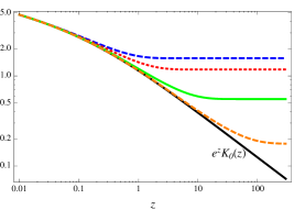
Figure 20: Comparison between the two sides of equation (143) for $n=1$, $2$, $10$ and $100$.

We now prove a useful relation between the hypergeometric function and the MacDonald function (modified Bessel function). If $\xi={\mbox{\large e}}^{-\frac{2z}{n}}\simeq 1-2z/n$, the integral (139) may be rewritten as

$$\int_{0}^{n}\frac{\mathrm{d}t}{n}\frac{\left(1-\frac{t}{n}\right)^{n-1/2}}{\sqrt{\frac{t}{n}\left(\frac{2z}{n}+\frac{t}{n}\right)}}\underset{n\to\infty}{\longrightarrow}\int_{0}^{\infty}\mathrm{d}t\,\frac{{\mbox{\large e}}^{-t}}{\sqrt{t(2z+t)}}\>.$$ (142)

We recognize an integral representation of the MacDonald function gragra . Therefore, for $z\ll n$, we can write

$$B\!\left(\frac{1}{2},n+\frac{1}{2}\right)\,F\!\left(\frac{1}{2},n+\frac{1}{2};n+1;{\mbox{\large e}}^{-\frac{2z}{n}}\right)\simeq{\mbox{\large e}}^{z}\,K_{0}(z)\>.$$ (143)

The r.h.s. describes the crossover between (140) and (141). We compare the two sides of equation (143) for different values of $n$ on figure 20.

Appendix D Laplace equation in networks : spectral determinant

In this appendix we introduce an important tool, the spectral determinant, used to study some properties of the equation

$$(\gamma-\Delta)P(x,x^{\prime})=\delta(x-x^{\prime})$$ (144)

in networks.

The spectral determinant is formally defined as $S(\gamma)=\det(\gamma-\Delta)=\prod_{n}(\gamma+E_{n})$ where $\{E_{n}\}$ is the spectrum of the Laplace operator $-\Delta$ (in the presence of a magnetic field, $\Delta\to[\nabla-2\mathrm{i}eA(x)]^{2}$). Despite this operator acts in a space of infinite dimension, the spectral determinant can be related to the determinant of a finite size matrix, of dimension equal to the number of vertices. This matrix encodes all informations on the network (topology, lengths of the wires, magnetic field, boundary conditions describing connections to reservoirs). Let us label vertices with greek letters. $l_{\alpha\beta}$ designates the length of the wire $({\alpha\beta})$ and $\theta_{\alpha\beta}$ the circulation of the vector potential along the wire. The topology is encoded in the adjacency matrix : $a_{\alpha\beta}=1$ if $\alpha$ and $\beta$ are linked by a wire, $a_{\alpha\beta}=0$ otherwise. We consider the case where Laplace operator acts on functions $\varphi(x)$ (i) continuous at the vertices satisfying (ii) $\sum_{\beta}{}a_{\alpha\beta}\varphi_{\alpha\beta}^{\prime}(0)=\lambda_{\alpha}\,\varphi_{\alpha}$ where $\varphi_{\alpha\beta}(x)$ designates the component of the function on the wire $({\alpha\beta})$ and $\varphi_{\alpha}$ its value at the vertex. Self-adjointness of the Laplace operator is ensured if $\lambda_{\alpha}\in{\ensmathonze R}$ (more details may be found in Refs. AkkComDesMonTex00 ; ComDesTex05 ). $\lambda_{\alpha}=\infty$ corresponds to Dirichlet boundary condition at the vertex and describe the case where $\alpha$ touches a reservoir through which current is injected in the network. $\lambda_{\alpha}=0$ for internal vertices. The interest of mixed boundary conditions (finite $\lambda_{\alpha}$) is illustrated in appendix F. We introduce the matrix

$$\mathcal{M}_{\alpha\beta} =\delta_{\alpha\beta}\left(\lambda_{\alpha}+\sqrt{\gamma}\sum_{\mu}a_{\alpha\mu}\coth\sqrt{\gamma}l_{\alpha\mu}\right)$$

$$\hskip 14.22636pt-a_{\alpha\beta}\,\sqrt{\gamma}\frac{{\mbox{\large e}}^{-\mathrm{i}\theta_{\alpha\beta}}}{\sinh\sqrt{\gamma}l_{\alpha\beta}}\>,$$ (145)

where the $a_{\alpha\mu}$ constrains the sum to run over neighbouring vertices. Then PasMon99 ; AkkComDesMonTex00

$$\boxed{S(\gamma)=\prod_{({\alpha\beta})}\frac{\sinh\sqrt{\gamma}l_{\alpha\beta}}{\sqrt{\gamma}}\>\det\mathcal{M}}$$ (146)

where the product runs over all wires. Despite the spectral determinant encodes the spectral information, it is also possible to extract some local information, like $P(x,x)$, by small modifications of the matrix. This has been used in Ref. TexMon05 and is briefly discussed in appendix F.

It is useful to remark that the matrix $\mathcal{M}$ can be used to express $P(x,x^{\prime})$ when $x$ and $x^{\prime}$ coincides with nodes (this is always possible to introduce a vertex anywhere without changing the properties of the network) :

$$\boxed{P(\alpha,\beta)=\left(\mathcal{M}^{-1}\right)_{\alpha\beta}}\>.$$ (147)

WL correction in regular networks.– In large regular networks connected in such a way that currents are uniformly distributed in the wires, we can assume that weights attributed to the wires of the networks in eq. (8) are equal. In this case, a uniform integration of the Cooperon $P_{c}(x,x)=\langle\kern 1.29167ptx\kern 1.29167pt|\frac{1}{\gamma-\Delta}|\kern 1.29167ptx\kern 1.29167pt\rangle$ in the network leads to a meaningful quantity (relevant experimentally). The Cooperon integrated uniformly is directly related to the spectral determinant Pas98 ; AkkComDesMonTex00

$$\int_{\mathrm{network}}\mathrm{d}{}x\>\Delta\tilde{\sigma}(x)=-2\,\frac{\partial}{\partial\gamma}\ln S(\gamma)\>.$$ (148)

This equation provides a very efficient way for calculating the WL correction in arbitrary networks, when uniform integration of Cooperon is justified.

WL correction in arbitrary networks.– In the most general case, eq. (8) requires to construct the Cooperon in each wire. A general expression was provided in TexMon04 however it is useful to notice that $P_{c}(x,x)$ can also be obtained from a spectral determinant for a modified boundary condition at point $x$. It was shown in Refs. TexMon05 ; ComDesTex05 that if we introduce mixed boundary conditions with a parameter $\lambda_{x}$ at $x$, then

$$P_{c}(x,x)=\frac{\partial}{\partial\lambda_{x}}\ln{S}^{(\lambda_{x})}(\gamma)\big{|}_{\lambda_{x}=0}\>.$$ (149)

Appendix E Classical resistance/conductance

We calculate the resistance between two vertices of an arbitrary network. We consider a network of wires of lengths $l_{\mu\nu}$ with same sections $s$. In this case the conductance of the wire $\mu\nu$ is given by $\sigma_{0}s/l_{\mu\nu}$. We introduce the matrix

$$(\mathcal{M}_{0})_{\mu\nu}=\delta_{\mu\nu}\sum_{\rho}\frac{a_{\mu\rho}}{l_{\mu\rho}}-\frac{a_{\mu\nu}}{l_{\mu\nu}}$$ (150)

whose matrix elements coincide with the conductances of the wires (up to the factor $\sigma_{0}s$). This matrix coincides with the matrix (D) if all fluxes are set to zero and the limit $\gamma\to 0$ is taken and moreover with $\lambda_{\mu}=0$, $\forall\>\mu$ for an isolated network.

We now consider the situation where we inject a current at the vertex $\alpha$. This current exits at vertex $\beta$ (see figure 21). If we denote by $V_{\mu}$ the potential at $\mu$, Kirchhoff law at vertex $\mu$ takes the form

$$\sigma_{0}s\sum_{\nu}(\mathcal{M}_{0})_{\mu\nu}V_{\nu}=I\,\left[\delta_{\mu,\alpha}-\delta_{\mu,\beta}\right]\>.$$ (151)

Potential is therefore given by :

$$V_{\mu}=\frac{I}{\sigma_{0}s}\left[(\mathcal{M}^{-1}_{0})_{\mu\alpha}-(\mathcal{M}^{-1}_{0})_{\mu\beta}\right]\>.$$ (152)

Note that the matrix $\mathcal{M}_{0}$ is not inversible ; it is explained below how to give a precise meaning to this expression. We define the resistance between points $\alpha$ and $\beta$ as $\mathcal{R}_{\alpha\beta}=(V_{\alpha}-V_{\beta})/I$. Therefore :

$$\mathcal{R}_{\alpha\beta}=\frac{2}{\sigma_{0}s}\left[\frac{(\mathcal{M}^{-1}_{0})_{\alpha\alpha}+(\mathcal{M}^{-1}_{0})_{\beta\beta}}{2}-(\mathcal{M}^{-1}_{0})_{\alpha\beta}\right]\>.$$ (153)

Using eq. (147) we see that we can express the resistance in terms of the solution $P_{d}$ of the equation $-\Delta{}P_{d}=\delta$ :

$$\boxed{\mathcal{R}(x,x^{\prime})=\frac{2}{\sigma_{0}s}\left[\frac{P_{d}(x,x)+P_{d}(x^{\prime},x^{\prime})}{2}-P_{d}(x,x^{\prime})\right]}$$

$$\hskip 42.67912pt=\frac{2}{\sigma_{0}s}\,W(x,x^{\prime})\>.$$ (154)

This demonstrates that the function $W(x,x^{\prime})$ defined by (17) is indeed the equivalent resistance between points $x$ and $x^{\prime}$.

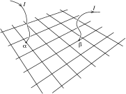
Figure 21: Injection of current in a network (here a regular square network).

Remark : $\mathcal{M}_{0}$ is not inversible.– It is easy to check that

$$\sum_{\mu}(\mathcal{M}_{0})_{\mu\nu}=0\>.$$ (155)

Kernel of the matrix is the vector $(1,1,\cdots,1)$. Physically eq. (155) ensures : (i) that sum of all currents arriving at vertex $\nu$ is zero, (ii) currents are zero if all potentials are equal (equilibrium). This problem can be overcome easily by noticing that only differences of inverse matrix elements have appeared, in eqs. (152) and (153). We can always inverse the matrix $\mathcal{M}_{0}$ in the space orthogonal to the vector $(1,1,\cdots,1)$ and compute differences of such matrix elements. This is how eqs. (152,153,E) must be understood.

In practice, an easier way to compute such differences is to regularize the calculation by computing the inverse of matrix $\mathcal{M}$ for finite $\gamma$ (or at least one finite $\lambda_{\alpha}$) and take the limit $\gamma\to 0$ (or $\lambda_{\alpha}\to 0$) after having computed the difference of inverse matrix elements :

$$(\mathcal{M}^{-1}_{0})_{\mu\alpha}-(\mathcal{M}^{-1}_{0})_{\mu\beta}=\lim_{\gamma\to 0}\left[\mathcal{M}^{-1}_{\mu\alpha}-\mathcal{M}^{-1}_{\mu\beta}\right]\>.$$ (156)

Note that $\det\mathcal{M}\neq 0$ for $\gamma\in{\ensmathonze R}^{+*}$ since $\mathrm{Spec}(\Delta)\subset{\ensmathonze R}^{-}$.

This point is related to the fact that was already mentioned in the continuum limit in order to construct the function $W(x,x^{\prime})$ (in section VIII.2.1 or in appendix F) : eq. (156) is the analogue of eq. (108). In the continuum this problem is related to the fact that the Laplace operator is not inversible in the space of functions satisfying Neumann boundary conditions corresponding to an isolated conductor.

Example : function $W$ in an isolated ring.– The relation between the function $W$ and the resistance may be used in order to construct easily $W$. Let us consider the case of a ring of perimeter $L$. When the ring is connected at two wires at $x$ and $x^{\prime}$, the resistance $\mathcal{R}(x,x^{\prime})$ corresponds to the one of two wires of lengths $|x-x^{\prime}|$ and $L-|x-x^{\prime}|$ put in parallel. We straightforwardly recover the function obtained in Ref. TexMon05b  :

$$W_{\mathrm{ring}}(x,x^{\prime}) =\frac{1}{2}\,\frac{1}{\frac{1}{|x-x^{\prime}|}+\frac{1}{L-|x-x^{\prime}|}}$$ (157)

$$=\frac{1}{2}\,|x-x^{\prime}|\left(1-\frac{|x-x^{\prime}|}{L}\right)\>.$$ (158)

Note that if we consider a ring connected at reservoirs through arms of finite length, the function $W(x,x^{\prime})$ inside the ring is modified LudMir04 ; TexMon05b , since its construction needs to consider a four terminal device. In the limit of infinitely long arms we can neglect currents flowing through the leads and we recover the result of the isolated ring (appendix of Ref. TexMon05b ).

Figure 22: A multiterminal network. Wavy lines represent contacts through which current is injected. Contacts correspond to vertices with primed labels.

Classical conductance.– It is interesting to compare the formula obtained for the resistance with the one obtained for the conductance matrix of a multiterminal network TexMon04 . We first stress that we consider two different situations. The eqs. (153,E) give the potentials when the currents injected at vertex $\alpha$ and extracted at vertex $\beta$ are fixed (figure 21). On the other hand, a conductance matrix allows to determine the currents through contacts when the potentials at these contacts are fixed (figure 22).

We consider a multiterminal network, connected to external contacts through which current is injected at a set of vertices indicated with primes : $\alpha^{\prime}$, $\beta^{\prime}$,… The connection is accounted for by introducing parameters $\lambda_{\alpha^{\prime}}=\infty$ added to the matrix $\mathcal{M}_{0}$, that now become inversible. These parameters describe Dirichlet conditions for the diffusion equation and permit to inverse the Laplace operator. The transport through the network is characterized by a conductance matrix whose elements are given by TexMon04

$$\mathcal{G}_{\alpha^{\prime}\beta^{\prime}}=-\frac{\sigma_{0}s}{l_{\alpha\alpha^{\prime}}l_{\beta\beta^{\prime}}}(\mathcal{M}^{-1}_{0})_{\alpha\beta}=-\frac{\sigma_{0}s}{l_{\alpha\alpha^{\prime}}l_{\beta\beta^{\prime}}}\,P_{d}(\alpha,\beta)\>.$$ (159)

At first sight diffuson $P_{d}(\alpha,\beta)$ (i.e. inverse matrix element $(\mathcal{M}^{-1}_{0})_{\alpha\beta}$) is related to both the conductance and the resistance. Note however that the matrix $\mathcal{M}_{0}$ (and the corresponding diffuson $P_{d}(x,x^{\prime})$) in eq. (159) does account for the boundary conditions (Dirichlet boundary conditions at contacts, i.e. primed vertices) whereas $\mathcal{M}_{0}$ (and $P_{d}(x,x^{\prime})$) in eqs. (153,E) describe the isolated network.

Appendix F Solution of the diffusion equation in some particular networks

We consider the solution of the diffusion eq. (144) for the networks studied in this article.

F.1 The ring with one or several arms

We consider a ring of perimeter $L$ attached to an arm of length $b$ connected to a reservoir (i.e. with Dirichlet boundary condition at its end) and submitted to a magnetic field. The spectral determinant is TexMon05  :

$$S(\gamma)=\frac{2}{\sqrt{\gamma}}\sinh\sqrt{\gamma}b\left[\cosh\sqrt{\gamma}L_{\mathrm{eff}}-\cos\theta\right]$$ (160)

where the effective perimeter is given by

$$\cosh\sqrt{\gamma}L_{\mathrm{eff}}=\cosh\sqrt{\gamma}L+\frac{1}{2}\coth\sqrt{\gamma}b\sinh\sqrt{\gamma}L\>.$$ (161)

A systematic way for obtaining the spectral determinant of two subgraphs glued at one vertex from the spectral determinants of the subgraphs has been derived in Ref. Tex08 . This allow to recover easily eq. (160).

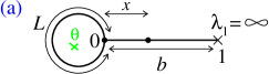
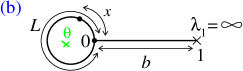
Figure 23: A ring with one wire. We choose a Dirichlet boundary condition at the vertex $1$ for simplicity ($\lambda_{1}=\infty$).

$\bullet$ Introducing mixed boundary conditions at the node (vertex $\mathrm{𝟎}$) we easily obtain $S^{(\lambda_{0})}(\gamma)=\frac{\lambda_{0}}{\gamma}\sinh\sqrt{\gamma}{}L\sinh\sqrt{\gamma}{}b+S(\gamma)$ from (146). Using eq. (149), and performing a Fourier transform, we get the Cooperon $P_{c}^{(n)}(0,0)=-\frac{1}{2}\Delta\tilde{\sigma}_{n}(0)$ at the node TexMon05

$$P_{c}^{(n)}(0,0)=\frac{1}{2\sqrt{\gamma}}\,\frac{\sinh\sqrt{\gamma}L}{\sinh\sqrt{\gamma}L_{\mathrm{eff}}}\,{\mbox{\large e}}^{-n\sqrt{\gamma}L_{\mathrm{eff}}}\>.$$ (162)

In the weakly coherent limit we find $L_{\mathrm{eff}}\simeq{}L+L_{\varphi}\ln(3/2)$, whence $P_{c}^{(n)}(0,0)\simeq\frac{1}{2\sqrt{\gamma}}\,\big{(}\frac{2}{3}\big{)}^{n+1}{\mbox{\large e}}^{-n\sqrt{\gamma}{}L}$.

In the limit $\sqrt{\gamma}L\ll 1$ the effective perimeter is $L_{\mathrm{eff}}\simeq\gamma^{-1/4}L^{1/2}$. We have TexMon05 ; ComDesTex05  :

$$P_{c}^{(n)}(0,0)\simeq\frac{\sqrt{L}}{2\gamma^{1/4}}\,{\mbox{\large e}}^{-n\sqrt{L}\gamma^{1/4}}\>.$$ (163)

$\bullet$ In order to calculate the harmonics of the Cooperon in the arm ($x$ is the distance from the ring, see figure 23.a), we have to consider the spectral determinant for the graph with mixed boundary conditions at $x$, with parameter $\lambda_{x}$ :

$$S^{(\lambda_{x})}(\gamma)=S(\gamma)+\frac{\lambda_{x}}{\gamma}\bigg{[}\sinh L\frac{\sinh^{2}(b-x)}{\sinh b}+2\sinh x\sinh(b-x)\left(\cosh L_{\mathrm{eff}}-\cos\theta\right)\bigg{]}$$ (164)

(for shorter notations we have omitted $\sqrt{\gamma}$ in hyperbolic functions). From eq. (149) we obtain :

$$\boxed{P_{c}^{(n)}(x,x)=\delta_{n,0}\frac{1}{\sqrt{\gamma}}\,\frac{\sinh\sqrt{\gamma}x\sinh\sqrt{\gamma}(b-x)}{\sinh\sqrt{\gamma}b}+\left(\frac{\sinh\sqrt{\gamma}(b-x)}{\sinh\sqrt{\gamma}b}\right)^{2}\,P_{c}^{(n)}(0,0)}$$ (165)

for $x\in$ arm (figure 23.a). We recognize the first term as the result obtained for a wire of length $b$ connected to reservoirs (i.e. with Dirichlet boundaries). In the limit $b\to\infty$ we have $P_{c}^{(n)}(x,x)\simeq P_{c}^{(n)}(0,0)\,{\mbox{\large e}}^{-2\sqrt{\gamma}x}$ (for $n\neq 0$).

$\bullet$ If $x$ is inside the ring (figure 23.b) the modified spectral determinant reads :

$$S^{(\lambda_{x})}(\gamma)=S(\gamma)+\frac{\lambda_{x}}{\gamma}\left[\sinh x\sinh(L-x)\cosh b+\sinh b\sinh L\right]$$ (166)

and from eq. (149) the Cooperon is therefore

$$\boxed{P_{c}^{(n)}(x,x)=\left[1+\coth\sqrt{\gamma}b\frac{\sinh\sqrt{\gamma}x\sinh\sqrt{\gamma}(L-x)}{\sinh\sqrt{\gamma}L}\right]\,P_{c}^{(n)}(0,0)}$$ (167)

for $x\in$ ring (figure 23.b).

If $L_{\varphi}\ll L$ we have $P_{c}^{(n)}(x,x)\simeq[\frac{3}{2}-\frac{1}{2}{\mbox{\large e}}^{-2\sqrt{\gamma}x}]P_{c}^{(n)}(0,0)$ for $x<L/2$. In the bulk (for $x$ and $L-x\gg L_{\varphi}$) we have $P_{c}^{(n)}(x,x)\simeq\frac{3}{2}P_{c}^{(n)}(0,0)$ (figure 24), where the factor $\frac{3}{2}$ corresponds to the ratio of coordination numbers at $\mathrm{𝟎}$ and at $x$.

In the opposite limit $L\ll L_{\varphi}\ll b$ the Cooperon is homogeneous inside the ring, as expected.

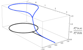
Figure 24: $x$ dependence of the Cooperon $P_{c}^{(n)}(x,x)$ in the connected ring for $L_{\varphi}\ll L$.

From one to $N_{a}$ arms.– In the regime $L_{\varphi}\ll{}L$, we have seen that the presence of one arm is responsible for factor $(\frac{2}{3})^{n}$ originating from the $n$ crossings of the vertex. We immediatly deduce that the Cooperon in the ring is $P_{c}^{(n)}(x,x)\simeq\frac{1}{2\sqrt{\gamma}}\,\big{(}\frac{2}{3}\big{)}^{nN_{a}}{\mbox{\large e}}^{-n\sqrt{\gamma}{}L}$.

In order to study the regime $L_{\varphi}\gg{}L$, instead of considering the network of figure 7 we discuss the case where all arms are attached at the same point in the ring. The calculation is more simple in this case. The two situations were studied in Ref. TexMon05 where it was shown that the Cooperons for the two networks only slightly differ in the regime $L_{\varphi}\ll{}L$ and are equal in the regime $L_{\varphi}\gg{}L$ of interest now. The effective length is now given by $\cosh\sqrt{\gamma}{}L_{\mathrm{eff}}=\cosh\sqrt{\gamma}{}L+\frac{N_{a}}{2}\sinh\sqrt{\gamma}{}L\,\coth\sqrt{\gamma}\,b$. The structure (162) still holds. When $L\ll{}L_{\varphi}\ll{}b$ we find $L_{\mathrm{eff}}\simeq\gamma^{-1/4}\sqrt{N_{a}L}$, therefore $P_{c}^{(n)}(x,x)\simeq\frac{1}{2}\sqrt{L_{\varphi}{}L/N_{a}}\,{\mbox{\large e}}^{-n\sqrt{N_{a}L/L_{\varphi}}}$, whose inverse Laplace transform leads to eq. (40). This $N_{a}$ dependence may be more simply obtained by noticing that, given the winding probability $\mathcal{P}_{n}(x,x;t)$ for one arm, the one for $N_{a}$ arms is obtained thanks to the substitution $n\to nN_{a}$ and $L\to{}L/N_{a}$.

F.2 The necklace of rings

We analyze the solution of the diffusion equation in a chain of $N_{r}$ identical rings of perimeter $L$. Rings are attached in such a way that the two arms joining two vertices are symmetric. The chain is closed in order to form a necklace for simplicity ; as soon as the total length is smaller than $L_{\varphi}$, the results are insensitive to boundary conditions : periodic (isolated necklace) or Dirichlet (chain connected to external contacts). Let us label the vertices joining consecutive rings with greek letters $\alpha,\,\beta\in\{1,\cdots,N_{r}\}$. The matrix introduced in appendix D has the simple form $\mathcal{M}_{\alpha\beta}=\frac{2\sqrt{\gamma}}{\sinh(\sqrt{\gamma}L/2)}\big{[}\delta_{\alpha\beta}\,2\cosh(\sqrt{\gamma}L/2)-a_{\alpha\beta}\,\cos(\theta/2)\big{]}$ where $\theta$ is the reduced flux per ring. With our convention the adjacency matrix reads $a_{\alpha\beta}=\delta_{\alpha,\beta+1}+\delta_{\alpha,\beta-1}$. Its spectrum of eigenvalues is $2\cos(2n\pi/N_{r})$ with $n\in\{1,\cdots,N_{r}\}$, therefore the spectral determinant reads :

$$S(\gamma) =\left(\frac{4\sinh(\sqrt{\gamma}L/2)}{\sqrt{\gamma}}\right)^{N_{r}}$$

$$\times\prod_{n=1}^{N_{r}}\left(\cosh(\sqrt{\gamma}L/2)-\cos(\theta/2)\cos\frac{2\pi n}{N_{r}}\right)\>.$$ (168)

We replace the product by a sum by considering the logarithm. The sum can then be computed in the limit $N_{r}\to\infty$ :

$$S(\gamma)\underset{N_{r}\to\infty}{=}\left(\frac{2|\cos(\theta/2)|\,\sinh(\sqrt{\gamma}L/2)}{\sqrt{\gamma}}\>{\mbox{\large e}}^{\mathop{\mathrm{argch}}\nolimits\left(\frac{\cosh(\sqrt{\gamma}L/2)}{|\cos(\theta/2)|}\right)}\right)^{N_{r}}\>.$$ (169)

We now consider $P(x,x^{\prime})$ when arguments coincide with vertices :

$$P(\alpha,\beta)=\left(\mathcal{M}\right)_{\alpha\beta}^{-1}=\frac{\sinh\sqrt{\gamma}L/2}{N_{r}4\sqrt{\gamma}}\sum_{n=1}^{N_{r}}\frac{{\mbox{\large e}}^{\frac{2\mathrm{i}\pi n}{N_{r}}(\alpha-\beta)}}{\cosh\sqrt{\gamma}L/2-\cos\frac{2\pi n}{N_{r}}}\underset{N_{r}\to\infty}{=}\frac{1}{4\sqrt{\gamma}}\,{\mbox{\large e}}^{-|\alpha-\beta|\sqrt{\gamma}L/2}\>.$$ (170)

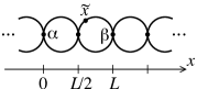
Figure 25: Infinite chain of rings.

We introduce the notation $\tilde{x}\equiv(x,f)$ to locate points in the chain, where $x$ is the coordinate along the axis (see figure) ; in the $n$-th ring $x\in[nL/2,(n+1)L/2]$. The discrete index $f\in\{u,d\}$ indicates whether the point is in the upper branch or the lower branch.

If $\tilde{x}$ and $\tilde{x}^{\prime}$ are arbitrary positions we can consider several situations.

$\bullet$ $\tilde{x}$ and $\tilde{x}^{\prime}$ belong to different rings. The Cooperon is

$$P(\tilde{x},\tilde{x}^{\prime})\simeq\frac{1}{4\sqrt{\gamma}}\,{\mbox{\large e}}^{-\sqrt{\gamma}|x-x^{\prime}|}\>,$$ (171)

that is half of the result for the infinite line.

$\bullet$ $\tilde{x}$ and $\tilde{x}^{\prime}$ belong to the same ring.

$$P(\tilde{x},\tilde{x}^{\prime})\underset{\gamma\to 0}{\simeq}\frac{1}{4\sqrt{\gamma}}\>.$$ (172)

We conclude that in time representation

$$\boxed{\mathcal{P}(\tilde{x},\tilde{x}^{\prime};t)\underset{t\gg L^{2}}{\simeq}\frac{1}{2}\,\frac{1}{\sqrt{4\pi t}}\,{\mbox{\large e}}^{-(x-x^{\prime})^{2}/4t}}$$ (173)

(the relation is exact when $\tilde{x}$ and $\tilde{x}^{\prime}$ belong to different rings). The $1/2$ corresponds to the probability to end in one of the two arms of the rings. It ensures normalisation : $\int\mathrm{d}\tilde{x}\,\mathcal{P}(\tilde{x},\tilde{x}^{\prime};t)\equiv\sum_{f=u,d}\int\mathrm{d}{x}\,\mathcal{P}(\tilde{x},\tilde{x}^{\prime};t)=1$.

The function $W(x,x^{\prime})$.– Expression (170) can be used to construct $P_{d}(x,x^{\prime})$ by taking the limit $\gamma\to 0$. We find for the function entering into description of dephasing :

$$W(x,x^{\prime})=\frac{1}{4}|x-x^{\prime}|=\frac{1}{2}W_{\mathrm{wire}}$$ (174)

for $x,\,x^{\prime}$ in different rings, and

$$W(x,x^{\prime})=\frac{1}{2}|x-x^{\prime}|\left(1-\frac{|x-x^{\prime}|}{L}\right)=W_{\mathrm{ring}}$$ (175)

for $x,\,x^{\prime}\in$ same ring. In (174) positions are measured along an axis along the chain ; the result is half of the result for a wire. As it has been already noticed this result can be understood thanks to the relation (E) : when the number of wires between each node is doubled, the resistance is divided by a factor of $2$. In (175) coordinates are relative to a unique axis inside the ring (it is understood that the expression is periodic) ; the result is exactly the result obtained for an isolated ring. Once again interpretation is easy : for an infinitely long necklace, when two external wires are plugged inside a ring, no current can flow out of the ring and resistance $\mathcal{R}(x,x^{\prime})$ is not affected by the remaining rings.

F.3 The square network

We construct the solution of the diffusion equation in the square network. We use (147) to express $P(x,x^{\prime})$ when the two coordinates coincide with nodes of the network. In this paragraph, nodes are labelled with a couple of integers $\alpha\to(n,m)\equiv\vec{R}$. The matrix $\mathcal{M}$ has the structure

$$\left(\mathcal{M}\right)_{\vec{R},\vec{R}\,^{\prime}}=\frac{\sqrt{\gamma}}{\sinh\sqrt{\gamma}a}\left[4\,\cosh\sqrt{\gamma}a\>\delta_{\vec{R},\vec{R}\,^{\prime}}-a_{\vec{R},\vec{R}\,^{\prime}}\right]\>.$$ (176)

This matrix is easily inverted

$$\left(\mathcal{M}^{-1}\right)_{\vec{R},\vec{R}\,^{\prime}} =\frac{\sinh\sqrt{\gamma}a}{2\sqrt{\gamma}}$$ (177)

$$\times\int_{\mathrm{ZdB}}\frac{\mathrm{d}\vec{Q}}{(2\pi)^{2}}\frac{{\mbox{\large e}}^{\mathrm{i}\vec{Q}\cdot(\vec{R}-\vec{R}\,^{\prime})}}{2\cosh\sqrt{\gamma}a-\cos Q_{x}-\cos Q_{y}}\>,$$

where integral runs over wavevectors of the Brillouin zone. If we are interested in $\mathcal{P}(x,x^{\prime};t)$ in the large time limit, $t\gg{}a^{2}$, this corresponds to consider $\gamma{}a^{2}\ll 1$. In this regime the above integral is dominated by small $\vec{Q}$ and we get

$$P(\vec{R},\vec{R}\,^{\prime}) =\left(\mathcal{M}^{-1}\right)_{\vec{R},\vec{R}\,^{\prime}}\simeq\frac{a}{2}\int\frac{\mathrm{d}\vec{Q}}{(2\pi)^{2}}\frac{{\mbox{\large e}}^{\mathrm{i}\vec{Q}\cdot(\vec{R}-\vec{R}\,^{\prime})}}{\gamma a^{2}+\frac{1}{2}\vec{Q}^{2}}$$

$$=\frac{a}{2}\int_{0}^{\infty}\mathrm{d}t\,{\mbox{\large e}}^{-\gamma t}\frac{1}{2\pi t}{\mbox{\large e}}^{-\frac{a^{2}}{2t}(\vec{R}-\vec{R}\,^{\prime})^{2}}$$ (178)

where integral over $\vec{Q}$ has been extended to ${\ensmathonze R}^{2}$. We expect $\mathcal{P}(x,x^{\prime};t)$ to vary smoothly on the scale of the lattice spacing, therefore we may write

$$\mathcal{P}(x,x^{\prime};t)\underset{t\gg a^{2}}{\simeq}\frac{a}{2}\,\frac{1}{2\pi t}{\mbox{\large e}}^{-\frac{1}{2t}||x-x^{\prime}||^{2}}$$ (179)

where $||x-x^{\prime}||$ designates the distance in ${\ensmathonze R}^{2}$ between the two points $x$ and $x^{\prime}$ of the square network. This result call for two remarks. First, we see that the fact that the diffusion is constrained in the 1d wires forming the square network leads to a continuum limit with a renormalized diffusion constant $D^{*}=1/2$, if the diffusion constant is $D=1$ in the wire (more generally $D^{*}=1/d$ where $d$ is the effective dimensionality of the network). Second, the probability presents a prefactor $1/2$ of similar origin than the one in eq. (173), ensuring normalization condition. Each elementary plaquette, labelled by $\vec{R}\equiv(n,m)$, contains 2 wires. Therefore each wire of the network can be labelled with $\vec{R}$ and an index $f$ taking two values (for horizontal or vertical wires). We check that (180) is correctly normalized : $\int_{\mathrm{network}}\mathrm{d}{}x\,\mathcal{P}(x,x^{\prime};t)=\sum_{\vec{R}}\sum_{f}\int_{\mathrm{wire}\>(\vec{R},f)}\mathrm{d}{}x\,\mathcal{P}(x,x^{\prime};t)\simeq\sum_{\vec{R}}2a\,\mathcal{P}(x,x^{\prime};t)\simeq 2a\sum_{\vec{R}}\frac{a}{2}\frac{1}{2\pi t}{\mbox{\large e}}^{-\frac{a^{2}}{2t}(\vec{R}-\vec{R}\,^{\prime})^{2}}\simeq 1$.

The generalization of (177,F.3,179) to the other regular planar networks can be done. We obtain :

$$\boxed{\mathcal{P}(x,x^{\prime};t)\underset{t\gg a^{2}}{\simeq}\frac{1}{2}\tan\left(\frac{\pi}{z}\right)\,\frac{a}{2\pi t}{\mbox{\large e}}^{-\frac{1}{2t}||x-x^{\prime}||^{2}}}$$ (180)

where the dimensionless factor $\frac{1}{2}\tan\frac{\pi}{z}$, where $z$ is the coordination number of the lattice, has the interpretation of the area of the Wigner-Seitz elementary cell $\mathcal{A}_{z}(1+\delta_{z,6})$, where $\mathcal{A}_{z}$ is defined in the next appendix, divided by the number of bonds per cell.

Appendix G MC of planar regular networks

G.1 Planar regular networks

We apply the formulae (146) and (148) to the case of infinite planar regular networks. Let us denote by $z$ the coordination number of the network. The plane can be covered by only three different tillings : the triangular lattice ($z=6$), the square lattice ($z=4$) and the honeycomb lattice ($z=3$).

Let us mention few properties of regular tillings of flat surfaces :

• the lattice of coordination number $z$ is a tilling by regular polygones with $p$ sides. $p$ is related to the coordination number by Sti92 $(z-2)(p-2)=4$.

• The area of a regular $p$-gone of side $a$ is $\mathcal{A}_{z}=a^{2}\frac{1}{4}p\mathop{\mathrm{cotg}}\nolimits(\pi/p)=a^{2}\frac{z}{2(z-2)}\tan(\pi/z)$.

• If boundary effects are neglected, the number of bonds $B$ and the number of vertices $V$ of the planar network are related by $2B=zV$ ($z$ bonds issue from each vertex and each bond touch 2 vertices).

The matrix (D) takes the form $\mathcal{M}=\frac{\sqrt{\gamma}}{\sinh\sqrt{\gamma}\,a}N$ where the matrix $N$ is given by

$$N_{\alpha\beta}=\delta_{\alpha\beta}\,z\,\cosh\sqrt{\gamma}\,a-a_{\alpha\beta}\,{\mbox{\large e}}^{-\mathrm{i}\theta_{\alpha\beta}}$$ (181)

where reduced fluxes $\theta_{\alpha\beta}$ describe a uniform magnetic field $\mathcal{B}$. We use eqs. (146,148) to express the WL correction $\Delta\tilde{\sigma}=-\frac{2}{\mathrm{Vol}}\frac{\partial}{\partial\gamma}\ln{}S(\gamma)$, where the volume is related to the number of bonds $\mathrm{Vol}=Ba$,

$$\Delta\tilde{\sigma}(\theta) =\left(\frac{2}{z}-1\right)\,L_{\varphi}\,\left(\coth\frac{a}{L_{\varphi}}-\frac{L_{\varphi}}{a}\right)$$

$$-\frac{z}{B}\,L_{\varphi}\,\sinh\frac{a}{L_{\varphi}}\,\mathop{\mathrm{Tr}}\nolimits\left\{\frac{1}{N(\gamma,\theta)}\right\}$$ (182)

$\theta=4\pi\phi/\phi_{0}$ is the reduced flux per elementary plaquette. The computation of this expression requires the knowledge of the spectrum of the matrix $N$, i.e. of $a_{\alpha\beta}\,{\mbox{\large e}}^{-\mathrm{i}\theta_{\alpha\beta}}$ (Hofstadter problem footnote18 ).

G.2 Continuum limit

We study the continuum limit : for $L_{\varphi}\gg{}a$ the WL correction probes large scales. Moreover when the flux per cell is much smaller that the flux quantum, $\phi\ll\phi_{0}$, the result for the planar network coincide with the result for a plane. Let us show that this is indeed the case. We note that the action of the adjacency matrix $a_{\alpha\beta}$ on a smooth function can be replaced by the Laplacian : $a_{\alpha\beta}\longrightarrow\frac{1}{4}za^{2}\,\Delta+z$. Therefore in the presence of a weak magnetic field $a_{\alpha\beta}\,{\mbox{\large e}}^{-\mathrm{i}\theta_{\alpha\beta}}\longrightarrow\frac{1}{4}za^{2}\,(\nabla-2\mathrm{i}\,eA)^{2}+z$ involves the covariant derivative. The spectrum of this operator is the Landau spectrum shifted by $-z$ : $\mathrm{Spec}(-a_{\alpha\beta}\,{\mbox{\large e}}^{-\mathrm{i}\theta_{\alpha\beta}})\simeq\{za^{2}e\mathcal{B}(n+1/2)-z\,|\,n\in{\ensmathonze N}\}$, where each Landau level has a degeneracy $d_{\mathrm{LL}}=\frac{1}{\pi}\,e\mathcal{B}\mathrm{Area}$, “$\mathrm{Area}$” being the total area occupied by the planar network.

In the limit $L_{\varphi}\gg{}a$ and $\theta\ll 1$, eq. (G.1) is dominated by the trace which is itself dominated by the bottom of the spectrum of $-a_{\alpha\beta}\,{\mbox{\large e}}^{-\mathrm{i}\theta_{\alpha\beta}}$ and it rewrites

$$\Delta\tilde{\sigma} \simeq-a\frac{z}{B}\,\frac{e\mathcal{B}\mathrm{Area}}{\pi}\,$$

$$\times\sum_{n=0}^{N_{c}}\frac{1}{z\frac{a^{2}}{2L_{\varphi}^{2}}+za^{2}e\mathcal{B}(n+1/2)}+\mathrm{cste}$$ (183)

where we have introduced a cutoff $N_{c}$ corresponding to the number of the Landau level for which continuum limit fails : $za^{2}e\mathcal{B}(N_{c}+1/2)\sim{}z$, the width of the spectrum of the adjacency matrix. This gives $N_{c}\sim 1/(a^{2}e\mathcal{B})\sim\phi_{0}/(\mathcal{B}a^{2})$. Using that the total number of bonds is related to the number of elementary plaquettes by $B=\frac{2z}{z-2}\frac{1}{2}\times(\#$ of plaquettes$)$ we find $\mathrm{Area}=\frac{a^{2}}{2}\tan(\pi/z)\>B$. Finally the WL correction may be expressed with the Digamma function gragra  :

$$\Delta\tilde{\sigma}(\theta\ll 1) \simeq\frac{a}{2\pi}\tan\left(\frac{\pi}{z}\right)$$ (184)

$$\times\left[\psi\!\left(\frac{1}{2}+\frac{\phi_{0}}{4\pi\mathcal{B}L_{\varphi}^{2}}\right)-\ln\left(\frac{\phi_{0}}{\mathcal{B}a^{2}}\right)\right]+\mathrm{cste}\>.$$

This result indeed coincides with the result for a plane, eq. (VII.2.1), apart for a factor $2$ in the argument of Digamma functions. We think that it is worth devoting a small paragraph to this point since it is related to some interesting property of the continuum limit of the result for the networks.

The additional factor of $2$ and the continuum limit.– As mentioned in section VII the WL correction in the network can be written with a path integral as

$$\Delta\tilde{\sigma}(\theta) =-2\int_{0}^{\infty}\mathrm{d}t\,{\mbox{\large e}}^{-t/L_{\varphi}^{2}}$$ (185)

$$\times\int_{x(0)=x}^{x(t)=x}\mathcal{D}x(\tau)\,{\mbox{\large e}}^{-\frac{1}{4}\int_{0}^{t}\mathrm{d}\tau\,\dot{x}^{2}+\mathrm{i}\theta\mathcal{N}[x(\tau)]}$$

where $\mathcal{N}[x(\tau)]$ is the (algebraic) number of elementary plaquettes surrounded the trajectories. When one is interested in large time scale properties ($t\gg{}a^{2}$), eq. (180) shows that the path integral over Brownian paths $x(\tau)$ in the square network can be replaced by a path integral over planar Brownian curves $\vec{r}(\tau)$ as

$$\int_{x(\tau)\in\mathrm{network}}\mathcal{D}x(\tau)\,{\mbox{\large e}}^{-\frac{1}{4}\int\mathrm{d}\tau\,\dot{x}^{2}}$$

$$\hskip 14.22636pt\to a\frac{1}{2}\tan\left(\frac{\pi}{z}\right)\int_{\vec{r}(\tau)\in\mathrm{plane}}\mathcal{D}\vec{r}(\tau)\,{\mbox{\large e}}^{-\frac{1}{2}\int\mathrm{d}\tau\,\dot{\vec{r}}\,^{2}}\>.$$ (186)

$\theta\mathcal{N}[x(\tau)]=2e\mathcal{B}\mathcal{A}[x(\tau)]$ coincides with the magnetic flux enclosed by the trajectory multiplied by $2e$, where $\mathcal{A}[x(\tau)]$ is the algebraic area enclosed by the curve ($\mathcal{A}[x(\tau)]=a^{2}\mathcal{N}[x(\tau)]$ for the square network). Finally we can rewrite (185) as

$$\Delta\tilde{\sigma}(\theta\ll 1) \simeq-a\tan\left(\frac{\pi}{z}\right)\int_{a^{2}}^{\infty}\mathrm{d}t\,{\mbox{\large e}}^{-t/L_{\varphi}^{2}}$$ (187)

$$\times\int_{\vec{r}(0)=\vec{r}}^{\vec{r}(t)=\vec{r}}\mathcal{D}\vec{r}(\tau)\,{\mbox{\large e}}^{-\frac{1}{4D^{*}}\int_{0}^{t}\mathrm{d}\tau\,\dot{\vec{r}}\,^{2}+2\mathrm{i}e\mathcal{B}\mathcal{A}[\vec{r}(\tau)]}$$

with $D^{*}=1/2$. Then we can use the well-known result Ber84 ; AkkMon07 (VII.2.1) to get $\Delta\tilde{\sigma}(\theta\ll 1)\simeq\frac{a}{2\pi}\tan(\frac{\pi}{z})\big{[}\psi\big{(}\frac{1}{2}+\frac{\phi_{0}}{8\pi\mathcal{B}D^{*}L_{\varphi}^{2}}\big{)}-\ln\big{(}\frac{\phi_{0}}{\mathcal{B}a^{2}}\big{)}\big{]}+$cste, which precisely coincides with (184).

G.3 Square network

The WL correction can be expressed more explicitely for rational fluxes. We recall briefly a derivation due to Douçot & Rammal DouRam86 for the case of a square network of dimension $V=N_{x}\times{N_{y}}$. We start from

$$\Delta\tilde{\sigma}(\theta) =-\frac{L_{\varphi}}{2}\bigg{[}\coth(\sqrt{\gamma}\,a)-\frac{1}{\sqrt{\gamma}\,a}$$ (188)

$$+4\sinh(\sqrt{\gamma}\,a)\>\frac{1}{N_{x}N_{y}}\,\mathop{\mathrm{Tr}}\nolimits\left\{\frac{1}{N(\gamma,\theta)}\right\}\bigg{]}\>.$$

We label the vertices $\alpha\equiv(n,m)$, $n$ for the position along the horizontal direction and $m$ along the vertical direction. We can choose a Landau gauge : $\theta_{\alpha\beta}=m\theta$ for horizontal wires, $\alpha\equiv(n,m)$ and $\beta\equiv(n+1,m)$, and $\theta_{\alpha\beta}=0$ for vertical wires.

The computation of the MC for a square network submitted to a magnetic field requires to consider the problem of determination of the spectrum of $H_{\alpha\beta}=-a_{\alpha\beta}{\mbox{\large e}}^{-\mathrm{i}\theta_{\alpha\beta}}$ (Hofstadter problem). In the Landau gauge where the flux is put along the $n$ axis the solution of $H\psi=\varepsilon\psi$ can be written as $\psi_{n,m}=\Phi_{m}{\mbox{\large e}}^{\mathrm{i}k_{x}n}$. We obtain the Harper equation $\Phi_{m-1}+[\varepsilon+2\cos(k_{x}+m\theta)]\Phi_{m}+\Phi_{m+1}=0$.

If the flux is rational $\theta_{p,q}=2\pi{p}/q$ with $p,\,q\in{\ensmathonze N}$, the Harper equation is periodic with periodicity $q$. Therefore, writing $m=r+qs$ with $s\in{\ensmathonze Z}$ and $r\in\{1,\cdots,q\}$ we can look for solutions of the form $\Phi_{m}=\varphi_{r}{\mbox{\large e}}^{\mathrm{i}k_{y}s}$. The wave function $\varphi_{r}$ is solution of a linear system $D_{q}\varphi=0$ where the hermitian $q\times{q}$-matrix $D_{q}$ is defined by

$$\left\{\begin{array}[]{llll}D_{r,r}&=&\varepsilon+2\cos\left(k_{x}+2\pi\frac{rp}{q}\right)&\mbox{for }r=1,\cdots,q\\ D_{r+1,r}&=&1&\mbox{for }r=1,\cdots,q-1\\ D_{q,1}&=&{\mbox{\large e}}^{\mathrm{i}k_{y}}&\end{array}\right.\>.$$ (192)

The secular equation $\det{D_{q}}=0$ gives the $q$ energy bands denoted $\varepsilon_{r}(\vec{k})$. Interestingly the secular equation can be rewritten as $\det{D_{q}}=(-1)^{q}[P_{p,q}(\varepsilon)-2(\cos qk_{x}+\cos k_{y})]=0$, where $P_{p,q}(\varepsilon)$ is a polynomial of degree ClaWan78 $q$. For example $P_{1,1}(\varepsilon)=-\varepsilon$, $P_{1,2}(\varepsilon)=\varepsilon^{2}-4$, $P_{1,3}(\varepsilon)=-\varepsilon^{3}+6\varepsilon$, etc.

The weak localization correction involves

$$\frac{1}{N_{x}N_{y}}\,\mathop{\mathrm{Tr}}\nolimits\left\{\frac{1}{N(\gamma,\theta_{p,q})}\right\}$$

$$=\int_{0}^{2\pi}\frac{\mathrm{d}^{2}\vec{k}}{(2\pi)^{2}}\>\frac{1}{q}\sum_{r=1}^{q}\frac{1}{4\cosh(\sqrt{\gamma}\,a)+\varepsilon_{r}(\vec{k})}$$ (193)

$$=\frac{1}{q}\,\int_{0}^{2\pi}\frac{\mathrm{d}^{2}\vec{k}}{(2\pi)^{2}}\,\frac{P^{\prime}_{p,q}(4\cosh(\sqrt{\gamma}\,a))}{P_{p,q}(4\cosh(\sqrt{\gamma}\,a))-2\cos k_{x}-2\cos k_{y}}\>,$$ (194)

where we have used the equality $\sum_{r=1}^{q}\frac{1}{\varepsilon-\varepsilon_{r}}=\frac{P^{\prime}(\varepsilon)}{P(\varepsilon)}$, valid for a polynomial of degree $q$ : $P(\varepsilon)=\prod_{r=1}^{q}(\varepsilon_{r}-\varepsilon)$. Integration over $\vec{k}$ leads to the result (75) of Douçot & Rammal.

References

- (1) S. Chakravarty and A. Schmid, Weak localization: the quasiclassical theory of electrons in a random potential, Phys. Rep. 140(4), 193 (1986).
- (2) E. Akkermans and G. Montambaux, Mesoscopic physics of electrons and photons, Cambridge University Press, 2007.
- (3) B. L. Altshuler, A. G. Aronov, and D. E. Khmelnitsky, Effects of electron-electron collisions with small energy transfers on quantum localisation, J. Phys. C: Solid State Phys. 15, 7367 (1982).
- (4) T. Ludwig and A. D. Mirlin, Interaction-induced dephasing of Aharonov-Bohm oscillations, Phys. Rev. B 69, 193306 (2004).
- (5) C. Texier and G. Montambaux, Dephasing due to electron-electron interaction in a diffusive ring, Phys. Rev. B 72(11), 115327 (2005) ; ibid 74, 209902(E) (2006).
- (6) M. Ferrier, A. C. H. Rowe, S. Guéron, H. Bouchiat, C. Texier, and G. Montambaux, Geometrical dependence of the decoherence due to electronic interactions in a GaAs/GaAlAs square network, Phys. Rev. Lett. 100(14), 146802 (2008).
- (7) C. Texier and G. Montambaux, Quantum oscillations in mesoscopic rings and anomalous diffusion, J. Phys. A: Math. Gen. 38, 3455–3471 (2005).
- (8) G. Montambaux and E. Akkermans, Non exponential quasiparticle decay and phase relaxation in low dimensional conductors, Phys. Rev. Lett. 95, 016403 (2005).
- (9) C. P. Umbach, C. van Haesendonck, R. B. Laibowitz, S. Washburn and R. A. Webb, Direct observation of Ensemble Averaging of the Aharonov-Bohm Effect in Normal Metal Loops, Phys. Rev. Lett. 56(4), 386 (1986).
- (10) S. Washburn and R. A. Webb, Aharonov-Bohm effect in normal metal. Quantum coherence and transport, Adv. Phys. 35(4), 375 (1986).
- (11) F. Schopfer, F. Mallet, D. Mailly, C. Texier, G. Montambaux, L. Saminadayar, and C. Bäuerle, Dimensional crossover in quantum networks: from mesoscopic to macroscopic physics, Phys. Rev. Lett. 98(2), 026807 (2007).
- (12) B. L. Al’tshuler and A. G. Aronov, Magnetoresistance of thin films and of wires in a longitudinal magnetic field, JETP Lett. 33(10), 499 (1981).
- (13) G. Bergmann, Weak localization in thin films, Phys. Rep. 107, 1 (1984).
- (14) B. L. Al’tshuler, A. G. Aronov, and B. Z. Spivak, The Aaronov-Bohm Effect in disordered conductors, JETP Lett. 33(2), 94 (1981).
- (15) A. G. Aronov and Yu. V. Sharvin, Magnetic flux effects in disordered conductors, Rev. Mod. Phys. 59(3), 755 (1987).
- (16) M. Ferrier, L. Angers, A. C. H. Rowe, S. Guéron, H. Bouchiat, C. Texier, G. Montambaux, and D. Mailly, Direct measurement of the phase coherence length in a GaAs/GaAlAs square network, Phys. Rev. Lett. 93(24), 246804 (2004).
- (17) D. Yu. Sharvin and Yu. V. Sharvin, Magnetic-flux quantization in a cylindrical film of a normal metal, JETP Lett. 34(5), 272 (1981).
- (18) B. L. Al’tshuler, A. G. Aronov, B. Z. Spivak, D. Yu. Sharvin, and Yu. V. Sharvin, Observation of the Aaronov-Bohm Effect in hollow metal cylinders, JETP Lett. 35(11), 588 (1982).
- (19) B. Pannetier, J. Chaussy, R. Rammal, and P. Gandit, Magnetic Flux Quantization in the Weak-Localization Regime of a Nonsuperconducting Metal, Phys. Rev. Lett. 53(7), 718 (1984).
- (20) B. Pannetier, J. Chaussy, R. Rammal, and P. Gandit, First Observation of Altshuler-Aronov-Spivak effect in gold and copper, Phys. Rev. B 31(5), 3209 (1985).
- (21) Amplitude of Aharonov-Bohm (AB) oscillations can be studied by analysis of the correlation function of the magnetoconductance. Therefore AB oscillations of the conductance (period ) are related to universal conductance fluctuations (UCF) while AAS oscillations of the averaged conductance (period ) are oscillations of the WL correction. See discussion in the appendix of Ref. TexMon05b .
- (22) F. Pierre and N. O. Birge, Dephasing by Extremely Dilute Magnetic Impurities Revealed by Aharonov-Bohm Oscillations, Phys. Rev. Lett. 89(20), 206804 (2002).
- (23) It was shown in Ref. TexMon05 on the case of the ring connected to arms that the crossover between the “small coherence length regime” and the “large coherence length regime” occurs in practice already for . The study of this regime is far from academic since in metallic samples can be made larger than m at mK, like in experiment BauMalSchMaiEskSam05 .
- (24) C. Bäuerle, F. Mallet, F. Schopfer, D. Mailly, G. Eska, and L. Saminadayar, Experimental Test of the Numerical Renormalization Group Theory for Inelastic Scattering from Magnetic Impurities, Phys. Rev. Lett. 95, 266805 (2005).
- (25) B. Douçot and R. Rammal, Quantum oscillations in normal-metal networks, Phys. Rev. Lett. 55(10), 1148 (1985).
- (26) B. Douçot and R. Rammal, Interference effects and magnetoresistance oscillations in normal-metal networks: 1. Weak localization approach, J. Physique 47, 973–999 (1986).
- (27) M. Pascaud, Magnétisme orbital de conducteurs mésoscopiques désordonnés et propriétés spectrales de fermions en interaction, PhD thesis, Université Paris 11, 1998.
- (28) M. Pascaud and G. Montambaux, Persistent currents on networks, Phys. Rev. Lett. 82, 4512 (1999).
- (29) E. Akkermans, A. Comtet, J. Desbois, G. Montambaux, and C. Texier, On the spectral determinant of quantum graphs, Ann. Phys. (N.Y.) 284, 10–51 (2000).
- (30) C. Texier and G. Montambaux, Weak localization in multiterminal networks of diffusive wires, Phys. Rev. Lett. 92(18), 186801 (2004).
- (31) This question was first considered in a ring in Ref. San89 who weighted properly the Cooperon in the wires. The rigorous proof and the generalization leading to a proper analysis of nonlocal effects was provided in Ref. TexMon04 .
- (32) P. Santhanam, Weak localization in normal-metal loops : Influence of boundary conditions, Phys. Rev. B 39(4), 2541 (1989).
- (33) B. L. Altshuler and A. G. Aronov, Electron-electron interaction in disordered conductors, in Electron-electron interactions in disordered systems, edited by A. L. Efros and M. Pollak, page 1, North-Holland, 1985.
- (34) Factors 2 are missing in the given in AAK’s original paper AleAltGer99 ; AkkMon07 .
- (35) I. L. Aleiner, B. L. Altshuler, and M. E. Gershenson, Interaction effects and phase relaxation in disordered systems, Waves Random Media 9, 201 (1999).
- (36) Let us estimate this length for the samples of Ref. SchMalMaiTexMonSamBau07 made of pure silver wires of width nm and thickness nm. Fermi wavelength in silver is nm (i.e. DoS is eV-1nm-3). This corresponds to channels. Diffusion constant was measured to be ms corresponding to elastic mean free path nm and leading to Km. We get Km.
- (37) Let us remind that is the localization length of the infinitely long wire Dor82 ; MelPerKum88 ; Bee97 . The perturbation theory is valid for AltAro85 (i.e. ), that is above the temperature .
- (38) O. N. Dorokhov, Transmission coefficient and the localization length of an electron in bound disordered chains, JETP Lett. 36, 318 (1982).
- (39) P. A. Mello, P. Pereyra, and N. Kumar, Macroscopic approach to multichannel disordered conductors, Ann. Phys. (N.Y.) 181, 290 (1988).
- (40) C. W. J. Beenakker, Random-Matrix theory of quantum transport, Rev. Mod. Phys. 69(3), 731–808 (1997).
- (41) F. Pierre, Interactions électron-électron dans les fils mésoscopiques, PhD thesis, Université Paris 6, 2000, Ann. Phys. (France) 26, (2001).
- (42) M. H. Pedersen, S. A. van Langen, and M. Büttiker, Charge fluctuations in quantum point contacts and chaotic cavities in the presence of transport, Phys. Rev. B 57(3), 1838 (1998).
- (43) K. Kobayashi, H. Aikawa, S. Katsumoto, and Y. Iye, Probe-Configuration-Dependent Decoherence in an Aharonov-Bohm Ring, J. Phys. Soc. Jpn. 71(9), L2094 (2002).
- (44) G. Seelig, S. Pilgram, A. N. Jordan, and M. Büttiker, Probe-configuration-dependent dephasing in a mesoscopic interferometer, Phys. Rev. B 68(16), 161310 (2003).
- (45) C. L. Kane, R. A. Serota, and P. A. Lee, Long-range correlations in disordered media, Phys. Rev. B 37(12), 6701 (1988).
- (46) S. Hershfield and V. Ambegaokar, Resistance fluctuations in a four probe geometry with infinite leads, Phys. Rev. B 38(12), 7909 (1988).
- (47) S. Hershfield, Current conservation and resistance fluctuations in a four probe geometry, Ann. Phys. (N.Y.) 196, 12 (1989).
- (48) M. B. Hastings, A. D. Stone, and H. U. Baranger, Inequivalence of weak localization and coherent backscattering, Phys. Rev. B 50(12), 8230 (1994).
- (49) S. Hikami, A. I. Larkin, and Y. Nagaoka, Spin-Orbit Interaction and Magnetoresistance in the Two Dimensional Random System, Prog. Theor. Phys. 63(2), 707 (1980).
- (50) The experiment Mal06 has investigated the regime where nonlocal effects are important, above K, when decoherence is dominated by electron-phonon scattering. The experimental MC was perfectly fitted by the MC obtained for a simple exponential relaxation.
- (51) F. Mallet, Effets de cohérence dans les fils et les réseaux quantiques. Étude de l’effet Kondo, PhD thesis, Université Joseph Fourier, Grenoble, 2006.
- (52) Note that the function involved in this functional may present a divergent behaviour at short distance : this is the case for the metallic film or the hollow cylinder studied in the last section for which . In this case one must come back to the assumption of classical electric fluctuations : due to the Pauli principle, energy transfers between electrons are limited to . This amounts to replace the Dirac of the correlator by a function of width : . The diverging term should be replaced by a term TreYevMarDelLer09 . Therefore the -function constrains the two trajectories to differ by at most the thermal length . This is the reason why it is sufficient to cut off the divergence of in at scale , according to Refs. AltAroKhm82 ; AltAro85 .
- (53) M. Treiber, O. M. Yevtushenko, F. Marquardt, J. von Delft, and I. V. Lerner, Dimensional Crossover of the dephasing time in disordered mesoscopic rings, preprint , arXiv:0905.1213 (2009).
- (54) Note that AAK’s treatment AltAroKhm82 of electron-electron interaction through some “influence functional” arising from the fluctuations of the classical electric field of the other electrons has initiated several works. A more sophisticated influence functional was constructed in Refs. MarDelSmiAmb07 ; DelMarSmiAmb07 where the quantum nature of the environment and the Pauli principle were accounted for, that justifies more rigorously the cutoff procedure of AAK (the difficulty lies in the fact that the “bath” -the other electrons- is of the same than the “system” -a given electron). The revival of this question was initiated by the work of Golubev & Zaikin GolZai98 ; GolZai99 . These authors have constructed an influence functional that correctly includes the Pauli principle MarDelSmiAmb07 , however their calculation within this basis, that has led to a finite decoherence rate at zero temperature, was later strongly criticized by several authors AleAltGer99 ; Imr02 ; see Refs. MarDelSmiAmb07 ; Del08 for a “neutral point of view” and detailed discussions.
- (55) F. Marquardt, J. von Delft, R. A. Smith, and V. Ambegaokar, Decoherence in weak localization. I. Pauli principle in influence functional, Phys. Rev. B 76(19), 195331 (2007).
- (56) J. von Delft, F. Marquardt, R. A. Smith, and V. Ambegaokar, Decoherence in weak localization. II. Bethe-Salpeter calculation of the cooperon, Phys. Rev. B 76(19), 195332 (2007).
- (57) D. S. Golubev and A. D. Zaikin, Quantum Decoherence in Disordered Mesoscopic Systems, Phys. Rev. Lett. 81(5), 1074 (1998).
- (58) D. S. Golubev and A. D. Zaikin, Quantum decoherence and weak localization at low temperatures, Phys. Rev. B 59(14), 9195 (1999).
- (59) Y. Imry, Elementary explanation of the inexistence of decoherence at zero temperature for systems with purely elastic scattering, preprint cond-mat/02 02 044 (2002).
- (60) J. von Delft, Influence Functional for Decoherence of Interacting Electrons in Disordered Conductors, Int. J. Mod. Phys. B 22, 727 (2008), cond-mat/05 10 563.
- (61) A. Comtet, J. Desbois, and C. Texier, Functionals of the Brownian motion, localization and metric graphs, J. Phys. A: Math. Gen. 38, R341–R383 (2005).
- (62) M. Abramowitz and I. A. Stegun, editors, Handbook of Mathematical functions, Dover, New York, 1964.
- (63) C. Texier, Effect of connecting wires on the decoherence due to electron-electron interaction in a metallic ring, Phys. Rev. B 76(15), 153312 (2007).
- (64) U. Sivan, Y. Imry, and A. G. Aronov, Quasiparticle lifetime in a quantum dot, Europhys. Lett. 28(2), 115 (1994).
- (65) M. Ferrier, Transport électronique dans les fils quasi-unidimensionnels : cohérence de phase dans les réseaux de fils quantiques et supraconductivité des cordes de nanotubes de carbone, PhD thesis, Université Paris-Sud, 2004.
- (66) G. J. Dolan, J. C. Licini, and D. J. Bishop, Quantum Interference Effects in Lithium Ring Arrays, Phys. Rev. Lett. 56(14), 1493 (1986).
- (67) I. S. Gradshteyn and I. M. Ryzhik, Table of integrals, series and products, Academic Press, fifth edition, 1994.
- (68) J.-P. Roth, Spectre du Laplacien sur un graphe, C. R. Acad. Sc. Paris 296, 793 (1983).
- (69) with .
- (70) C. Texier and G. Montambaux, Altshuler-Aronov correction to the conductivity of a large metallic square network, Phys. Rev. B 76(9), 094202 (2007).
- (71) D. C. Khandekar and F. W. Wiegel, Distribution of the area enclosed by a plane random walk, J. Phys. A: Math. Gen. 21, L563 (1988).
- (72) M. Yor, On stochastic areas and averages of planar Brownian motion, J. Phys. A: Math. Gen. 22, 3049 (1989).
- (73) B. Duplantier, Areas of planar Brownian curves, J. Phys. A: Math. Gen. 22, 3033 (1989).
- (74) A. Comtet, J. Desbois, and S. Ouvry, Winding of planar Brownian curves, J. Phys. A: Math. Gen. 23, 3563 (1990).
- (75) G. Montambaux, Comment on “Theory of electronic diamagnetism in two-dimensional lattices”, Phys. Rev. Lett. 63(15), 1657 (1989).
- (76) J. Bellissard, C. J. Camacho, A. Barelli, and F. Claro, Exact random walk distributions using noncommutative geometry, J. Phys. A: Math. Gen. 30, L707 (1997).
- (77) J. Desbois, unpublished (2008).
- (78) In Ref. AltAro85 a distinction between inelastic and “quasielastic” processes is made. The former refer to high energy transfers (however limited by the Pauli principle) while the latter stands for low energy transfers. This separation is motivated by the low energy divergences in the usual perturbative treatment Eil84 . This has led AAK to propose the influence functional approach AltAroKhm82 . We however insist on the fact that the influence functional approach fully account for electron-electron interaction, what is clear on the more sophisticated version MarDelSmiAmb07 ; DelMarSmiAmb07 , and not only to quasielastic processes.
- (79) W. Eiler, Electron-electron interaction and weak localisation, J. Low Temp. Phys. 56(5/6), 481 (1984).
- (80) A quantity frequently introduced is , the “dimensionless conductance” (of a square connected at two opposite sides). In a plane (2DEG), the sheet resistance reads , where is the effective mass of charge carriers. In a thin film of thickness , it is given by where is the DoS per volume and per spin channel. LEt us give order of magnitude : for a film of silver of thickness nm with nm we obtain .
- (81) P. M. Echternach, M. R. Thoman, C. M. Gould, and H. M. Bozler, Electron-phonon scattering rates in disordered metallic films below 1 K, Phys. Rev. B 46(16), 10339 (1992).
- (82) M. Eshkol, E. Eisenberg, M. Karpovski, and A. Palevski, Dephasing time in a two-dimensional electron Fermi liquid, Phys. Rev. B 73, 115318 (2006).
- (83) . The“return probability” is given by where “energies” correspond to the spectrum of : for a degeneracy , therefore . Using formula [3.541] of Ref. gragra , gives (VII.2.1).
- (84) We recall limiting behaviours gragra : for large and for small ; C.
- (85) Note that this procedure can be avoided by computing the Cooperon beyond the diffusion approximation (by solving the Bethe-Salpether integral equation) as it has been discussed in Ref. DmiKacGor97 (these authors have extended a previous work CasSha94 where some contributions were forgotten).
- (86) A. P. Dmitriev, V. Y. Kachorovskii, and I. V. Gornyi, Nonbackscattering contribution to weak localization, Phys. Rev. B 56(15), 9910 (1997).
- (87) A. Cassam-Chenai and B. Shapiro, Two dimensional weak localization beyond the diffusion approximation, J. Phys. I France 4, 1527 (1994).
- (88) for the silver samples of Refs. SchMalMaiTexMonSamBau07 ; Mal06 the factor is therefore (compared to for the film). From ms we obtain m at K. Therefore the various Nyquist lengths are Km for the infinite wire, Km for the 2d film and Km for the square network.
- (89) C. Texier, On the spectrum of the Laplace operator of metric graphs attached at a vertex – Spectral determinant approach, J. Phys. A: Math. Theor. 41, 085207 (2008).
- (90) J. Stillwell, Geometry of Surfaces, Springer-Verlag, 1992.
- (91) F. Claro and G. H. Wannier, Closure of bands for Bloch electrons in a magnetic field, Phys. Status Solidi B 88, K147 (1978).
- (92) An equality in law relates two processes with similar statistical properties.
- (93) Note that if we have and .
- (94) The Landau problem on a lattice was solved by Hofstadter Hof76 on the square lattice, by Claro & Wannier ClaWan79 on the triangular lattice and on the honeycomb lattice by Rammal Ram85 . Note however that Hofstadter butterflies were already plotted in an older paper by Langbein Lan69 (see also GerLan66 ).
- (95) D. R. Hofstadter, Energy levels and wave functions of Bloch electrons in rational and irrational magnetic fields, Phys. Rev. B 14(6), 2239 (1976).
- (96) F. H. Claro and G. H. Wannier, Magnetic structure of electrons in hexagonal lattices, Phys. Rev. B 19(12), 6068 (1979).
- (97) R. Rammal, Landau spectrum of Bloch electrons in a honeycomb lattice, J. Physique 46, 1345 (1985).
- (98) D. Langbein, The Tight-Binding and the Nearly-Free-Electron Approach to Lattice Electrons in External Magnetic Fields, Phys. Rev. 180(3), 633 (1969).
- (99) E. Gerlach and D. Langbein, Tight-Binding Approach to Electrons in a Crystal Potential and an External Magnetic Field, Phys. Rev. 145(2), 449 (1966).