Direct mapping between exchange potentials of Hartree-Fock and Kohn-Sham schemes as origin of orbitals proximity

Abstract

It is found that, in closed-$l$-shell atoms, the exact local exchange potential $v_{\text{x}}(\bf r)$ of the density functional theory (DFT) is very well represented, within the region of every atomic shell, by each of the suitably shifted potentials obtained with the non-local Fock exchange operator for the individual Hartree-Fock (HF) orbitals belonging to this shell. Consequently, the continuous piecewise function built of shell-specific exchange potentials, each defined as the weighted average of the shifted orbital exchange potentials corresponding to a given shell, yields another highly-accurate representation of $v_{\text{x}}(\bf r)$. These newly revealed properties are not related to the well-known step-like shell structure in the response part of $v_{\text{x}}(\bf r)$, but they result from specific relations satisfied by the HF orbital exchange potentials. These relations explain the outstanding proximity of the occupied Kohn-Sham and HF orbitals as well as the high quality of the Krieger-Li-Iafrate and localized HF (or, equivalently, common-energy-denominator) approximations to the DFT exchange potential $v_{\text{x}}(\bf r)$. The constant shifts added to the HF orbital exchange potentials, to map them onto $v_{\text{x}}(\bf r)$, are nearly equal to the differences between the energies of the corresponding KS and HF orbitals. It is discussed why these differences are positive and grow when the respective orbital energies become lower for inner orbitals.

I INTRODUCTION

Representing the quantum state of a many-electron system in terms of one-electron orbitals is simple and theoretically attractive approach. Such description is realized in the Hartree-Fock (HF) method johnson07 , as well as in the Kohn-Sham (KS) scheme of the density-functional theory (DFT) PY89 ; DG91 ; FN03 . The latter is an efficient and robust tool which is now routinely applied in the calculations of electronic properties of molecules, even very large and complex, and condensed-matter structures. Though the KS scheme is formally accurate, the one-body KS potential contains the exchange-correlation (xc) potential $v_{\text{xc}}$, whose exact dependence on the electron density remains unknown. It is usually treated within the local-density or generalized-gradient approximations (LDA, GGA), despite the well-known shortcomings of the LDA and GGA xc potentials (especially the self-interaction errors). Some of these deficiencies are removed when the exact form (in terms of the occupied KS orbitals) is used for the exchange part $E_{\text{x}}$ of the xc energy. The exact exchange potential $v_{\text{x}}$ is then found from $E_{\text{x}}$ by means of the integral equation resulting from the optimized-effective-potential (OEP) approach [KLI92, (a),EV93, ; GKKG00, ; E03, ; KK08, ] or by using the recently developed method based on the differential equations for the orbital shifts KP03 ; CH07 ; another method based on the direct energy minimization with respect to the KS-OEP potential (expressed in a finite basis) YW02 suffers from convergence problems SSD06 which are not fully resolved yet and they are still under studyHBBY07 ; HBY08 . The exact potential $v_{\text{x}}$ is free from self-interaction and it has correct asymptotic dependence ($-1/r$ for finite systems) at large distances $r$ from the system; thus, unlike the HF, LDA or GGA potentials, it produces correct unoccupied states. In the DFT, the approximation, in which the exchange is included exactly but the correlation energy and potential are neglected, is known as the exchange-only KS scheme — it is applied in the present investigation. The full potential $v_{\text{xc}}$ can also be found by means of the OEP approach when the DFT total energy includes, besides the exact $E_{\text{x}}$, the correlation energy $E_{\text{c}}$ depending on all (occupied and unoccupied) KS orbitals and orbital energies E03 . This makes such computation tedious, to a level undesirable in the DFT, since it involves calculating $E_{\text{c}}$ with the quantum-chemistry methods, like the Møller-Plesset many-body perturbation approach.

Defined to yield the true electron density, the KS one-electron orbitals have no other direct physical meaning since they formally refer to a fictitious system of non-interacting electrons. However, it is a common practice to use these orbitals in calculations of various electronic properties; in doing so the $N$-electron ground-state wave function $\Psi_{0}$ of the physical (interacting) system is approximated with the single determinant built of the KS orbitals. This approximate approach is justified by (usually) sufficient accuracy of the calculated quantities, which is close to, or often better than, that of the HF results Bour00 . It seems that the success of the DFT calculations would not be possible if the KS determinant, though being formally non-physical, was not close to the HF determinant which, outside the DFT, is routinely used to approximate the wave function $\Psi_{0}$ of the real system. Therefore, understanding this proximity is certainly very important for the fundamentals of the DFT.

Previous calculations [KLI92, (a),ZP92_93, ; Nagy93, ; CES94, ] have shown that, not only the whole KS and HF determinants Bour00 ; DSG01 and the corresponding electron densities [KLI92, (a),GE95, ; SMVG97, ; SMMVG99, ], but also the individual occupied KS and HF orbitals, $\phi_{a\sigma}({\bf r})$ and $\phi_{a\sigma}^{\text{HF}}({\bf r})$, in atoms are so close to each other that they are virtually indistinguishable (here the orbitals, dependent on the electron position $\bf r$ and the spin $\sigma=\downarrow$, $\uparrow$, are numbered with index $a=1,\ldots,N_{\sigma}$; $N_{\downarrow}+N_{\uparrow}=N$). This property is particularly remarkable for the exchange-only KS orbitals which differ so minutely from the HF orbitals that, for atoms, the OEP total energy is only several mhartrees higher than the HF energy $E_{\text{HF}}$ KLI92 ; EV93 ; KK08 ; GE95 . The outstanding proximity of the KS and HF orbitals is surprising in view of the obvious difference between the exchange operators in the KS and HF one-electron hamiltonians (see below) and the fact that the corresponding KS and HF atomic orbital energies, $\epsilon_{a\sigma}$ and $\epsilon_{a\sigma}^{\text{HF}}$, differ substantially, up to several hartrees for core orbitals in atoms like Ar, Cu EV93 ; KK08 [except for the KS and HF energies of the highest-occupied molecular orbital (HOMO) which are almost identical]. This apparent contradiction has not yet been resolved; in Ref. IL03 it is suggested that the KS and HF determinants are close to each other “since the kinetic energy is much greater than the magnitude of the exchange energy”.

The present paper investigates the proximity of the KS and HF orbitals and it reveals that, in closed-$l$-shell atoms, there exists a direct mapping between the HF orbital local exchange potentials $v_{\text{x}a\sigma}^{\text{HF}}({\bf r})$ and the DFT exact local exchange potential $v_{\text{x}\sigma}({\bf r})$. The former are specific to each HF orbital $\phi_{a\sigma}^{\text{HF}}({\bf r})$ and are defined as

$$v_{\text{x}a\sigma}^{\text{HF}}({\bf r})\equiv\frac{\hat{v}_{\text{x}\sigma}^{\text{F}}\phi_{a\sigma}^{\text{HF}}({\bf r})}{\phi_{a\sigma}^{\text{HF}}({\bf r})}\;$$ (1)

with the Fock exchange non-local operator $\hat{v}_{\text{x}\sigma}^{\text{F}}({\bf r})$ within the HF approximation that describes the interacting system. The DFT exchange potential $v_{\text{x}\sigma}({\bf r})$ is common for all orbitals relevant to the KS non-interacting $\sigma$ subsystem. This potential is found to be very well represented, within the region of each atomic shell, by the individual, suitably shifted potentials $\tilde{v}_{\text{x}a\sigma}^{\text{HF}}({\bf r})=v_{\text{x}a\sigma}^{\text{HF}}({\bf r})+C_{a\sigma}$ obtained for the HF orbitals that belong to this shell; the constant shifts $C_{a\sigma}$ are orbital-specific. As a result, for each shell, the weighted average of the potentials $\tilde{v}_{\text{x}a\sigma}^{\text{HF}}({\bf r})$ corresponding to the orbitals from this shell yields the shell-specific exchange potential that also represents $v_{\text{x}\sigma}({\bf r})$ with high accuracy within the shell region. The revealed mapping between $\tilde{v}_{\text{x}a\sigma}^{\text{HF}}({\bf r})$ and $v_{\text{x}\sigma}({\bf r})$ is shown to have origins in the specific relations satisfied by the HF orbital exchange potentials. Thus, the proximity of the KS and HF orbitals is explained. Simultaneously, it becomes clear why, in atoms, the exact exchange potential $v_{\text{x}\sigma}(r)$ (where $r=|{\bf r}|$) has the characteristic structure of a piecewise function where each part spans over the region of an atomic shell and it has distinctively different slope $dv_{\text{x}\sigma}(r)/dr$ in consecutive shells leeuwen96 .

The specific properties of $v_{\text{x}a\sigma}^{\text{HF}}({\bf r})$ are also shown to be directly responsible for the high quality of the approximate representations of the exact exchange potential $v_{\text{x}\sigma}({\bf r})$ that are obtained in the Krieger-Li-Iafrate(KLI) KLI92 and localized HF (LHF)DSG01 approximations, the latter of which is equivalent to the common-energy-denominator approximation (CEDA) GB01 . The constant shifts $C_{a\sigma}$, needed to map the HF potentials $v_{\text{x}a\sigma}^{\text{HF}}({\bf r})$ onto $v_{\text{x}\sigma}({\bf r})$, are shown to be nearly equal to $\epsilon_{a\sigma}-\epsilon_{a\sigma}^{\text{HF}}$. This leads to better understanding why, for each KS occupied orbital (other than the HOMO), its energy $\epsilon_{a\sigma}$ is higher than the corresponding HF energy $\epsilon_{a\sigma}^{\text{HF}}$ and the difference between these two energies is larger for the core orbitals than for the valence ones. Finally, it is shortly argued that the presently revealed properties of the KS and HF exchange potentials do not result from the well-known step-like shell structure present in the response part $v_{\text{x}\sigma}^{\text{resp}}({\bf r})$ of the exchange potential leeuwen94 ; leeuwen95 .

II THEORY

II.1 Hartree-Fock method and optimized-effective-potential approach

The HF one-electron spin-orbitals $\phi_{a\sigma}^{\text{HF}}(\bf r)$ are obtained by minimizing the mean value $\langle\Psi|\hat{H}|\Psi\rangle$ where $\hat{H}$ is the Hamiltonian of the $N$-electron interacting system and $\Psi$ belongs to the subspace $\Omega_{N}^{\text{det}}$ of normalized $N$-electron wave functions that are single Slater determinants built of one-electron orbitals. Similar minimization is carried out in the exchange-only OEP method, but there is the additional constraint that for every trial determinant all $N_{\sigma}$ constituent spin-orbitals $\phi_{a\sigma}({\bf r})$ satisfy the KS equation with some local KS potential $v_{\text{s}\sigma}({\bf r})$. The minimizing potential $v_{\text{s}\sigma}({\bf r})=v_{\text{s}\sigma}^{\text{OEP}}({\bf r})$, yields, after subtracting from it the external $v_{\text{ext}}({\bf r})$ and electrostatic $v_{\text{es}}({\bf r})$ terms, the exact exchange potential $v_{\text{x}\sigma}({\bf r})=v_{\text{x}\sigma}^{\text{OEP}}({\bf r})$ (corresponding to the density $n_{\sigma}$ calculated from occupied $\phi_{a\sigma}$), so that we have

$$v_{\text{s}\sigma}({\bf r})=v_{\text{ext}}({\bf r})+v_{\text{es}}({\bf r})+v_{\text{x}\sigma}({\bf r})\,.$$ (2)

It has to be stressed here that the proximity of the exchange-only KS and HF orbitals is not readily implied by the fact the two sets of orbitals result from the minimization of the same functional of energy, i.e., $E[\Psi]=\langle\Psi|\hat{H}|\Psi\rangle$ where $\Psi\in\Omega_{N}^{\text{det}}$. Indeed, for a suitably chosen model Hamiltonian $\hat{H}$, the corresponding HF orbitals $\phi_{a\sigma}^{\text{HF}}({\bf r})$ that minimize $E[\Psi]$ might not be well approximated by any set of one-electron (KS) orbitals $\phi_{a\sigma}({\bf r})$ that come from a common local potential $v_{\text{s}\sigma}({\bf r})$. Then, the latter condition, which is imposed on the orbitals $\phi_{a\sigma}({\bf r})$ in the OEP minimization, would be so restrictive that the obtained KS-OEP orbitals would differ significantly from the HF ones. Thus, it seems that it is the specific form of the physical Hamiltonian $\hat{H}$ (with Coulombic interactions) that actually makes the close representation of the HF orbitals with the KS ones possible.

The exchange-only KS equation, satisfied by the corresponding (OEP) orbitals $\phi_{a\sigma}({\bf r})$ and their energies $\epsilon_{a\sigma}$, takes the form

$$\hat{h}_{\text{s}\sigma}({\bf r})\phi_{a\sigma}({\bf r})\equiv\Bigl{[}-\frac{1}{2}\bm{\nabla}^{2}+v_{\text{ext}}({\bf r})+v_{\text{es}}({\bf r})+v_{\text{x}\sigma}({\bf r})\Bigr{]}\phi_{a\sigma}({\bf r})=\epsilon_{a\sigma}\phi_{a\sigma}({\bf r})$$ (3)

(atomic units are used throughout) where we put $v_{\text{x}\sigma}({\bf r})=v_{\text{x}\sigma}^{\text{OEP}}({\bf r})$ in the OEP case. The total electron density $n_{\text{tot}}({\bf r})=n_{\uparrow}({\bf r})+n_{\downarrow}({\bf r})$, which enters

$$v_{\text{es}}[n_{\text{tot}}]({\bf r})=\int d\,{\bf r^{\prime}}\,\frac{n_{\text{tot}}({\bf r^{\prime}})}{|{\bf r^{\prime}-r}|}\,,$$ (4)

is the sum of the spin-projected densities

$$n_{\sigma}({\bf r})=\sum_{a=1}^{N_{\sigma}}|\phi_{a\sigma}({\bf r})|^{2}\,.$$ (5)

In the HF equation

$$\hat{h}_{\text{HF}\sigma}({\bf r})\phi_{a\sigma}^{\text{HF}}({\bf r})\equiv\Bigl{[}-\frac{1}{2}\bm{\nabla}^{2}+v_{\text{ext}}({\bf r})+v_{\text{es}}^{\text{HF}}({\bf r})+\hat{v}_{\text{x}\sigma}^{\text{F}}({\bf r})\Bigr{]}\phi_{a\sigma}^{\text{HF}}({\bf r})=\epsilon_{a\sigma}^{\text{HF}}\phi_{a\sigma}^{\text{HF}}({\bf r})\,,$$ (6)

satisfied by the orbitals $\phi_{a\sigma}^{\text{HF}}(\bf r)$ and energies $\epsilon_{a\sigma}^{\text{HF}}$, the multiplicative local exchange potential $v_{\text{x}\sigma}({\bf r})$, present in the KS equation (3), is replaced with the non-local Fock exchange integral operator $\hat{v}_{\text{x}\sigma}^{\text{F}}({\bf r})$, built of $\{\phi_{a\sigma}^{\text{HF}}\}_{a=1}^{N_{\sigma}}$; its action on a given HF orbital $\phi_{a\sigma}^{\text{HF}}$ yields johnson07

$$\hat{v}_{\text{x}\sigma}^{\text{F}}\left[\{\phi_{b\sigma}^{\text{HF}}\}\right]\!({\bf r})\,\phi_{a\sigma}^{\text{HF}}({\bf r})=-\sum_{b=1}^{N_{\sigma}}\phi_{b\sigma}^{\text{HF}}({\bf r})\int d{\bf r^{\prime}}\,\frac{\phi_{b\sigma}^{\text{HF}}({\bf r}^{\prime})\phi_{a\sigma}^{\text{HF}}({\bf r}^{\prime})}{|{\bf r}^{\prime}-{\bf r}|}\,.$$ (7)

The electrostatic potential $v_{\text{es}}^{\text{HF}}({\bf r})=v_{\text{es}}[n_{\text{tot}}^{\text{HF}}]({\bf r})$ is found for the HF total electron density $n_{\text{tot}}^{\text{HF}}({\bf r})$ defined in a similar way as $n_{\text{tot}}({\bf r})$. The KS and HF orbitals are ordered according to non-descending values of the corresponding orbital energies ( $\epsilon_{a\sigma}\leq\epsilon_{a+1,\sigma}\,$ and $\epsilon_{a\sigma}^{\text{HF}}\leq\epsilon_{a+1,\sigma}^{\text{HF}}$, $a=1,\ldots$). Both the KS and HF equations need to be solved selfconsistently. Real KS and HF orbitals are used throughout this paper.

Obviously, for each HF orbital $\phi_{a\sigma}^{\text{HF}}(\bf r)$, the Fock exchange operator $\hat{v}_{\text{x}\sigma}^{\text{F}}({\bf r})$ present in the HF equation (6) can be formally replaced by $v_{\text{x}a\sigma}^{\text{HF}}({\bf r})$, Eq. (1), however, this local exchange potential is orbital-dependent due the non-locality of $\hat{v}_{\text{x}\sigma}^{\text{F}}({\bf r})$, Eq. (7). Thus, also, the resulting total HF potential

$$v_{\text{s}a\sigma}^{\text{HF}}({\bf r})=v_{\text{ext}}({\bf r})+v_{\text{es}}^{\text{HF}}({\bf r})+v_{\text{x}a\sigma}^{\text{HF}}({\bf r})$$ (8)

is different for each orbital $\phi_{a\sigma}^{\text{HF}}({\bf r})$, unlike in the KS scheme where all electrons (of given spin $\sigma$) are subject to the same total potential $v_{\text{s}\sigma}({\bf r})$, which includes the common exchange potential $v_{\text{x}\sigma}({\bf r})$. Dependence on $\sigma$ will be suppressed hereafter (unless otherwise stated).

II.2 Orbital and energy shifts. Exact exchange potential

The exact exchange potential $v_{\text{x}}=v_{\text{x}}^{\text{OEP}}$ satisfies the OEP equation GKKG00 ; KP03

$$\delta n({\bf r})\equiv 2\sum_{a=1}^{N}\phi_{a}({\bf r})\delta\phi_{a}({\bf r})=0\;,\;\;\forall{\bf r}\;,$$ (9)

which results from the OEP minimization and depends on $v_{\text{x}}$ through the orbital shifts (OS) $\delta\phi_{a}({\bf r})$. Each OS fulfills the equation GKKG00 ; KP03 ; CH07

$$\Bigl{[}\hat{h}_{\text{s}}({\bf r})-\epsilon_{a}\Bigr{]}\delta\phi_{a}({\bf r})=W_{a}^{\perp}({\bf r})$$ (10)

(where $\phi_{a}$, $\epsilon_{a}$ are the solutions of Eq. (3)) and it is subject to the constraint $\langle\phi_{a}|\delta\phi_{a}\rangle=0$. The equation (10) includes the KS Hamiltonian $\hat{h}_{\text{s}}$, present in Eq. (3), and the term (defined using the sign convention of Refs. KP03, ; CH07, )

$$W_{a}^{\perp}({\bf r})=\left[\hat{v}_{\text{x}}^{\text{F}}({\bf r})+D_{aa}-v_{\text{x}}({\bf r})\right]\phi_{a}({\bf r})\,.$$ (11)

where $\hat{v}_{\text{x}}^{\text{F}}=\hat{v}_{\text{x}}^{\text{F}}\left[\{\phi_{b}\}\right]$ and

$$D_{aa}=\langle\phi_{a}|v_{\text{x}}-\hat{v}_{\text{x}}^{\text{F}}|\phi_{a}\rangle\,.$$ (12)

It should be noted that $\int d{\bf r}\,\phi_{a}({\bf r})W_{a}^{\perp}({\bf r})=0$.

The OS $\delta\phi_{a}$ and the energy shift (ES) – the constant $D_{aa}$ give, within the perturbation theory (PT), the first-order approximations to the orbital and energy differences (shifts), $-(\tilde{\phi}_{a}^{\,\text{HF}}-\phi_{a})$ and $-(\tilde{\epsilon}_{a}^{\,\text{HF}}-\epsilon_{a})$, respectively. Here, the orbitals $\tilde{\phi}_{a}^{\,\text{HF}}$ and the corresponding energies $\tilde{\epsilon}_{a}^{\,\text{HF}}$, are the solutions of the HF-like equation which is the same as Eq. (3) except for $v_{\text{x}}$ replaced by $\hat{v}_{\text{x}}^{\text{F}}$ built of the KS orbitals $\{\phi_{b}\}$. The corresponding perturbation is then equal to $\delta\hat{h}_{\text{s}}=\hat{v}_{\text{x}}^{\text{F}}-v_{\text{x}}$ so that the first-order correction to $\epsilon_{a}$ is $-\delta\epsilon_{a}=\langle\phi_{a}|\delta\hat{h}_{\text{s}}|\phi_{a}\rangle=-D_{aa}$ while the correction to $\phi_{a}({\bf r})$ is

$$-\delta\phi_{a}({\bf r}) = \sum_{j=1,\epsilon_{j}\neq\epsilon_{a}}^{\infty}c_{ja}\,\phi_{j}({\bf r})\,,$$ (13)

$$c_{ja} = \frac{D_{ja}}{\epsilon_{j}-\epsilon_{a}}\,,$$ (14)

$$D_{ja} = -\langle\phi_{j}|\delta\hat{h}_{\text{s}}|\phi_{a}\rangle=\langle\phi_{j}|v_{\text{x}}-\hat{v}_{\text{x}}^{\text{F}}|\phi_{a}\rangle\,.$$ (15)

It satisfies Eq. (10) and the constraint $\langle\phi_{a}|\delta\phi_{a}\rangle=0$ indeed. Obviously, the solutions $\tilde{\phi}_{a}^{\,\text{HF}}$, $\tilde{\epsilon}_{a}^{\,\text{HF}}$ are not identical to the selfconsistent HF orbitals $\phi_{a}^{\text{HF}}$ and orbital energies $\epsilon_{a}^{\text{HF}}$ which are obtained from Eq. (6). The latter HF quantities can also be found within the PT approach by calculating the differences $\Delta\phi_{a}\equiv\phi_{a}^{\text{HF}}-\phi_{a}$, $\Delta\epsilon_{a}\equiv\epsilon_{a}^{\text{HF}}-\epsilon_{a}$ in the first-order approximation. In this case, the perturbation is given by $\Delta\hat{h}_{\text{s}}=\hat{h}_{\text{HF}}-\hat{h}_{\text{s}}$ [where $\hat{h}_{\text{HF}}$ is the HF Hamiltonian of Eq. (6)] and it consists of three terms, $\Delta\hat{h}_{\text{s}}=\delta\hat{h}_{\text{s}}+\Delta v_{\text{es}}+\Delta\hat{v}_{\text{x}}^{\text{F}}\;$. The terms $\Delta v_{\text{es}}=v_{\text{es}}[n_{\text{tot}}^{\text{HF}}]-v_{\text{es}}[n_{\text{tot}}]=v_{\text{es}}[n_{\text{tot}}^{\text{HF}}-n_{\text{tot}}]$ (cf. Eq. (4)) and $\Delta\hat{v}_{\text{x}}^{\text{F}}=\hat{v}_{\text{x}}^{\text{F}}[\{\phi_{a}^{\text{HF}}\}]-\hat{v}_{\text{x}}^{\text{F}}[\{\phi_{a}\}]$ depend on $\Delta\phi_{a}$ (of both spins for $\Delta v_{\text{es}}$), linearly in the leading order, so that they have to be calculated selfconsistently even in the PT approach. But, if we substitute $(-\delta\phi_{a})$ for $\Delta\phi_{a}$ the difference $n_{\text{tot}}^{\text{HF}}-n_{\text{tot}}$ becomes $\delta n_{\uparrow}+\delta n_{\downarrow}$ so that it vanishes due to the OEP equation (9). Then, we find $\Delta v_{\text{es}}=0$ and the perturbation $\Delta\hat{h}_{\text{s}}$ becomes $\delta\hat{h}_{\text{s}}+\Delta\hat{v}_{\text{x}}^{\text{F}}\left[\{\phi_{a}\},\{\delta\phi_{a}\}\right]$. It can be further reduced to $\delta\hat{h}_{\text{s}}$ if the OS $\delta\phi_{a}$ are sufficiently small. This argument, although not strict, leads to the conclusion that the differences $\Delta\phi_{a}$ and $\Delta\epsilon_{a}$ are well represented by the orbital and energy shifts, $-\delta\phi_{a}$ and $-\delta\epsilon_{a}=-D_{aa}$, respectively, which are obtained with the perturbation $\delta\hat{h}_{\text{s}}$. This conclusion is confirmed by the relations $\|\Delta\phi_{a}-(-\delta\phi_{a})\|<0.13\|\Delta\phi_{a}\|$ (where $\|\phi\|^{2}=\int d{\bf r}\,|\phi({\bf r})|^{2}$) and $|\Delta\epsilon_{a}-(-\delta\epsilon_{a})|<0.003|\Delta\epsilon_{a}|$ note-diff-en , established numerically for the Be and Ar atoms (see Tables 1 and 2); the above inequalities are obtained for $\phi_{a}$, $\epsilon_{a}$, $\delta\phi_{a}$ calculated as in Ref. CH07 , and $\phi_{a}^{\text{HF}}$ (expanded in the Slater-type-orbital basis), $\epsilon_{a}^{\text{HF}}$ taken from Ref. bunge93 . The representations of $\phi_{a}^{\text{HF}}-\phi_{a}$ by $-\delta\phi_{a}$ and $\epsilon_{a}^{\text{HF}}-\epsilon_{a}$ by $-\delta\epsilon_{a}$ will be used in further discussion. They can also be applied to construct a nearly accurate approximation of the exact exchange potential; the new method will be reported elsewhere soon CH09 .

The part of $W_{a}({\bf r})\equiv\delta\hat{h}_{\text{s}}({\bf r})\phi_{a}({\bf r})$ parallel to the orbital $\phi_{a}$ is

$$W_{a}^{||}({\bf r})=-D_{aa}\phi_{a}({\bf r})$$ (16)

and it sets the ES $\delta\epsilon_{a}=D_{aa}$. The part

$$W_{a}^{\perp}({\bf r})=W_{a}({\bf r})-W_{a}^{||}({\bf r})\,,$$ (17)

perpendicular to $\phi_{a}$, sets the OS $\delta\phi_{a}({\bf r})$, Eqs. (10), (11). Thus, the KS and HF orbitals, $\phi_{a}({\bf r})$, $\phi_{a}^{\text{HF}}({\bf r})$, can be close to each other, even if the orbital energies $\epsilon_{a}$, $\epsilon_{a}^{\text{HF}}$, differ significantly, provided the term $W_{a}^{\perp}({\bf r})$ is sufficiently small. Note that the orbitals remain unchanged when a (possibly orbital-dependent) constant is added to the Hamiltonian in the KS or HF equations.

When the equation (10) (after multiplying it by $\phi_{a}({\bf r})$ and subsequent summing over $a=1,\ldots,N$) is combined with the OEP condition (9), the following expression GKKG00 ; KP03 ; CH07 for the exact exchange potential is obtained

$$v_{\text{x}}^{\text{OEP}}({\bf r})=\breve{v}_{\text{x}}^{\text{KLI}}({\bf r})+v_{\text{x}}^{\text{OS}}({\bf r})$$ (18)

It contains the KLI-like potential KLI92

$$\breve{v}_{\text{x}}^{\text{KLI}}\left[\{\phi_{a}\},\{D_{aa}\}\right]({\bf r})=v_{\text{x}}^{\text{Sl}}({\bf r})+v_{\text{x}}^{\text{ES}}({\bf r})$$ (19)

which consists of the Slater potential

$$v_{\text{x}}^{\text{Sl}}({\bf r})=\frac{1}{n({\bf r})}\sum_{a=1}^{N}\phi_{a}({\bf r})\hat{v}_{\text{x}}^{\text{F}}({\bf r})\phi_{a}({\bf r})$$ (20)

and the ES term, linear in $D_{aa}$,

$$v_{\text{x}}^{\text{ES}}({\bf r})=\frac{1}{n({\bf r})}\sum_{a=1}^{N}D_{aa}\phi_{a}^{2}({\bf r})$$ (21)

where $n({\bf r})=\sum_{a=1}^{N}\phi_{a}^{2}({\bf r})$ ; these terms are defined with the OEP orbitals $\phi_{a}({\bf r})$ and constants $D_{aa}$. The OS term present in Eq. (18), linear in $\delta\phi_{a}({\bf r})$, is

$$v_{\text{x}}^{\text{OS}}({\bf r})=\frac{1}{n({\bf r})}\sum_{a=1}^{N}\bigl{[}2\epsilon_{a}\phi_{a}({\bf r})-\bigl{(}\bm{\nabla}\phi_{a}({\bf r})\bigr{)}\!\cdot\!\bm{\nabla}\bigr{]}\delta\phi_{a}({\bf r})\,.$$ (22)

Since any physical potential is defined up to an arbitrary constant, it is usually chosen that the constant $D_{NN}=0$ for the HOMO KP03 ; then the potential $v_{\text{x}}^{\text{OEP}}({\bf r})$ goes to 0 as $-1/r$ for $r=|{\bf r}|\rightarrow\infty$ (except for the directions that lie within symmetry planes in some molecules: in this special case the $(-1/r+{\text{const}})$ dependence at large $r$ is found; cf. Ref. KP03, ; DSG02, ).

However, the use of Eq. (18) for calculation of $v_{\text{x}}^{\text{OEP}}({\bf r})$ still requires solving the equations (9,10) for $\delta\phi_{a}({\bf r})$ as well as determining the selfconsistent values of the constants $D_{aa}$ which depend on $v_{\text{x}}=v_{\text{x}}^{\text{OEP}}({\bf r})$ through Eq. (12). This solution is obtained in an iterative way in Ref. KP03, , while a non-iterative algorithm, where both sets $\{\delta\phi_{a}\}$ and $\{D_{aa}\}$ are found simultaneously, is presented in Ref. CH07, . Let us note that the equations (9-12), (18-22) can be used to determine the exact exchange potential $v_{\text{x}}^{\text{OEP}}({\bf r})$ not only in the exchange-only OEP approach, but also when the orbitals $\phi_{a}({\bf r})$ are the solutions of the KS equation with the potential $v_{\text{s}}({\bf r})$ that, besides $v_{\text{x}}({\bf r})$, includes a correlation term $v_{\text{c}}({\bf r})$.

II.3 High-quality KLI and LHF (CEDA) approximations

Since the OS $\delta\phi_{a}({\bf r})$ are usually small, the term $v_{\text{x}}^{\text{OS}}({\bf r})$, Eq. (22), is a minor correction to $v_{\text{x}}^{\text{KLI}}({\bf r})$ in Eq. (18). Therefore, when we neglect $v_{\text{x}}^{\text{OS}}({\bf r})$ completely, the exact exchange potential $v_{\text{x}}^{\text{OEP}}({\bf r})$ is represented with high quality by the KLI-like term $\breve{v}_{\text{x}}^{\text{KLI}}({\bf r})$, Eq. (19). The original KLI approximation KLI92

$$v_{\text{x}}^{\text{KLI}}\left[\{\phi_{a}\}\right]({\bf r})=\breve{v}_{\text{x}}^{\text{KLI}}\left[\{\phi_{a}\},\{D_{aa}^{\text{KLI}}\}\right]({\bf r})$$ (23)

is obtained (here for the KS-OEP orbitals $\phi_{a}$) when the constants

$$D_{aa}^{\text{KLI}}=\langle\phi_{a}|v_{\text{x}}^{\text{KLI}}-\hat{v}_{\text{x}}^{\text{F}}|\phi_{a}\rangle$$ (24)

are found selfconsistently, analogously as $D_{aa}$ in Eq. (12) for $v_{\text{x}}=v_{\text{x}}^{\text{OEP}}$. Since, the equation (24) remains satisfied when an arbitrary constant, but the same for all $a$, is added to each $D_{aa}^{\text{KLI}}$, one usually sets $D_{NN}^{\text{KLI}}=0$ which makes the potential $v_{\text{x}}^{\text{KLI}}({\bf r})$ decay like $-1/r$ for large $r$.

The sum over $j$ in Eq. (13) can be split into two terms,

$$\delta\phi_{a}^{\text{occ}} = -\sum_{b=1,b\neq a}^{N}c_{ba}\,\phi_{b}\,,$$ (25)

$$\delta\phi_{a}^{\text{vir}} = -\sum_{t=N+1}^{\infty}c_{ta}\,\phi_{t}\,,$$ (26)

which are the projections of the OS $\delta\phi_{a}$ onto the subspaces of occupied (occ) and virtual (vir) orbitals, respectively. Thus, the OS term $v_{\text{x}}^{\text{OS}}({\bf r})$, Eq. (22), can be rewritten as follows

$$v_{\text{x}}^{\text{OS}}({\bf r})=\frac{1}{n({\bf r})}\sum_{a=1}^{N-1}\sum_{b=a+1}^{N}2D_{ab}\phi_{a}({\bf r})\phi_{b}({\bf r})+v_{\text{x}}^{\text{OS,vir}}({\bf r})$$ (27)

after the definition (14) of $c_{ta}$ and relation $D_{ba}=D_{ab}$ [cf. Eq. (15), $v_{\text{x}}^{\text{F}}$ is Hermitian and real] are used; the term

$$v_{\text{x}}^{\text{OS,vir}}({\bf r})=v_{\text{x}}^{\text{OS}}\left[\{\phi_{a}\},\{\epsilon_{a}\},\{\delta\phi_{a}^{\text{vir}}\}\right]({\bf r})$$ (28)

is found by substituting $\delta\phi_{a}^{\text{vir}}$ for $\delta\phi_{a}$ in Eq. (22). When the OS $\delta\phi_{a}$ are small, the corresponding projected parts $\delta\phi_{a}^{\text{vir}}$ are even smaller since the general relation $\|\delta\phi_{a}^{\text{occ}}\|^{2}+\|\delta\phi_{a}^{\text{vir}}\|^{2}=\|\delta\phi_{a}\|^{2}$ holds. Then, another high-quality representation of $v_{\text{x}}^{\text{OEP}}$

$$\breve{v}_{\text{x}}^{\text{LHF}}\left[\{\phi_{a}\},\{D_{ab}\}\right]({\bf r})=v_{\text{x}}^{\text{Sl}}({\bf r})+\frac{1}{n({\bf r})}\sum_{a,b=1}^{N}D_{ab}\phi_{a}({\bf r})\phi_{b}({\bf r})$$ (29)

is obtained by setting $\delta\phi_{a}^{\text{vir}}({\bf r})=0$ in the OS term $v_{\text{x}}^{\text{OS}}({\bf r})$, Eqs. (27, 28). This representation yields the well-known LHF (CEDA) approximation GB01 ; DSG01

$$v_{\text{x}}^{\text{LHF}}\left[\{\phi_{a}\}\right]=\breve{v}_{\text{x}}^{\text{LHF}}\left[\{\phi_{a}\},\{D_{ab}^{\text{LHF}}\}\right]$$ (30)

(here defined for the set $\{\phi_{a}\}$ of the KS-OEP orbitals) when the constants $D_{ab}^{\text{LHF}}=\langle\phi_{a}|v_{\text{x}}^{\text{KLI}}-\hat{v}_{\text{x}}^{\text{F}}|\phi_{b}\rangle\,,$ defined analogously as in Eq. (15), are found selfconsistently for $(ab)\neq(NN)$; we also set $D_{NN}^{\text{LHF}}=0$, as in the KLI case. Let us note that the condition $\delta\phi_{a\sigma}^{\text{vir}}=0$ is equivalent to the relation $\tilde{\phi}_{a\sigma}^{\text{HF}}=\phi_{a\sigma}+\sum_{b\neq a}^{\text{occ}}c_{ba}\phi_{b\sigma}$ (valid in the first-order approximation) which, when satisfied for both spins $\sigma$, implies that the HF determinant built of $\{\tilde{\phi}_{a\sigma}^{\text{HF}}\}$ is identical to the KS determinant built of $\{\phi_{a\sigma}\}$. This (approximate) identity has been assumed in Ref. DSG01, to derive the LHF approximation. Obviously, both the KLI and LHF approximate exchange potentials can be defined for any set of (orthogonal, bound) orbitals $\{\phi_{a}\}_{a=1}^{N}$. In particular, it can be done for the orbitals that are selfconsistent solutions of the KS equation (3) where the potential $v_{\text{x}}$ is set to $v_{\text{x}}^{\text{KLI}}\left[\{\phi_{a}\}\right]$ or $v_{\text{x}}^{\text{LHF}}\left[\{\phi_{a}\}\right]$.

The high quality of the KLI and LHF approximate potentials, when derived as presented above, clearly results from the proximity of the HF and KS-OEP occupied orbitals which is characterized by the small OS $\delta\phi_{a}$. However, the OS terms $v_{\text{x}}^{\text{OS}}$ and $v_{\text{x}}^{\text{OS,vir}}$ which are neglected in the KLI and LHF (CEDA) approximations, respectively, are expressed through all OS $\delta\phi_{a}$ (or their projected parts $\delta\phi_{a}^{\text{vir}}$). As a result, some information associated with the small magnitudes of the individual OS $\delta\phi_{a}$ may be lost in the resulting potentials $v_{\text{x}}^{\text{KLI}}$ and $v_{\text{x}}^{\text{LHF}}$. In particular, the Slater term, Eq. (20), present in these potentials, can be viewed the weighted average

$$v_{\text{x}}^{\text{Sl}}({\bf r})=\sum_{a=1}^{N}v_{\text{x}a}({\bf r})\frac{\phi_{a}^{2}({\bf r})}{n({\bf r})}$$ (31)

of the KS orbital exchange potentials

$$v_{\text{x}a}({\bf r})=\frac{\hat{v}_{\text{x}}^{\text{F}}({\bf r})\phi_{a}({\bf r})}{\phi_{a}({\bf r})}\,,$$ (32)

so that it cannot fully reflect the properties of the individual $v_{\text{x}a}({\bf r})$. In the following discussion (Sec. III) for closed-$l$-subshell atoms, new properties of $v_{\text{x}a}({\bf r})$ are exposed only when the proximity of the HF and KS-OEP orbitals is considered separately for each orbital.

II.4 Closed-$l$-subshell atoms: Fock exchange operator, orbital exchange potentials

For a closed-$l$-subshell atom, the non-local (integral) Fock exchange operator, acting on an atomic orbital $\phi_{a}({\bf r})=r^{-1}\chi_{nl}(r)Y_{lm}(\theta,\varphi)$ ($a\equiv nlm$), yields

$$\hat{v}_{\text{x}}^{\text{F}}({\bf r})\phi_{a}({\bf r})=r^{-1}F_{\text{x};nl}(r)\,Y_{lm}(\theta,\phi)$$ (33)

where $Y_{lm}(\theta,\varphi)$ is the spherical harmonic, Hereafter, the orbitals are labeled with the principal, orbital, and magnetic quantum numbers, $n$, $l$, $m$; the symbols $n_{\text{occ}}$ and $l_{\text{max}}^{(n)}$ will denote, respectively, the largest number $n$ and the maximum value of $l$ for given $n$, within the set $\{\text{occ}\}$ of the occupied orbitals $\{\phi_{nlm}\}$ (hereafter, we refer to this set with the general label ”occ”). It will be convenient to have a notation for the HOMO label: $H\equiv(n\,l_{\text{max}}^{(n)})$ at $n=n_{\text{occ}}$; note that the HOMO belongs to the outmost occupied shell for the closed-$l$-shell atoms. The factor

$$F_{\text{x};nl}(r)=\sum_{n^{\prime}l^{\prime}}^{\text{occ}}\sum_{l^{\prime\prime}=|l-l^{\prime}|}^{l+l^{\prime}}g(l,l^{\prime},l^{\prime\prime})\chi_{n^{\prime}l^{\prime}}(r)\,v_{l^{\prime\prime}}(n^{\prime}l^{\prime},nl;r)\,,$$ (34a)

is defined johnson07 (here with the occupied KS radial orbitals $$\chi_{n^{\prime}l^{\prime}}(r)\,$$) through the functions

$$v_{l^{\prime\prime}}(n^{\prime}l^{\prime},nl;r)=-\int_{0}^{\infty}dr^{\prime}\frac{(r_{<})^{l^{\prime\prime}}}{(r_{>})^{l^{\prime\prime}+1}}\chi_{n^{\prime}l^{\prime}}(r^{\prime})\chi_{nl}(r^{\prime})$$ (34b)

where we denote $g(l,l^{\prime},l^{\prime\prime})=(2l^{\prime}+1)\left(\begin{array}[]{c c c}l&l^{\prime}&l^{\prime\prime}\\ 0&0&0\\ \end{array}\right)$ (a special case of the $3j$ Wigner symbol), $r_{<}=\min(r,r^{\prime})$, $r_{>}=\max(r,r^{\prime})$. In particular, the following non-zero coefficients $g(0,0,0)=1$, $g(0,1,1)=1$, $g(1,1,0)=1$, $g(1,0,1)=1/3$, $g(1,1,2)=2/5$ are needed to find the quantities $F_{\text{x};nl}(r)$ for atoms with $s$ and $p$ orbitals (like Be, Ar); note that the step in the summation over $l^{\prime\prime}$ in Eq. (34a) is 2. Thus, the orbital exchange potential, Eq. (32),

$$v_{\text{x}a}({\bf r})=v_{\text{x};nl}(r)=F_{\text{x};nl}(r)/\chi_{nl}(r)\,,$$ (35)

is obtained; the corresponding HF quantities, denoted as $v_{l^{\prime\prime}}^{\text{HF}}(n^{\prime}l^{\prime},nl;r)$, $F_{\text{x};nl}^{\text{HF}}(r)$, $v_{\text{x}a}^{\text{HF}}({\bf r})=v_{\text{x};nl}^{\text{HF}}(r)$, can be determined with the HF atomic radial orbitals $\chi_{nl}^{\text{HF}}(r)$. The OS

$$\delta\phi_{a}({\bf r})=r^{-1}\delta\chi_{nl}(r)Y_{lm}(\theta,\varphi)$$ (36)

depends on the term

$$W_{a}^{\perp}({\bf r})=r^{-1}W_{nl}^{\perp\text{;rad}}(r)Y_{lm}(\theta,\varphi)$$ (37)

through its radial part

$$W_{nl}^{\perp;\text{rad}}(r)=F_{\text{x};nl}(r)+\left[D_{nl;nl}-v_{\text{x}}(r)\right]\chi_{nl}(r)$$ (38)

entering the equation

$$\left[-\frac{1}{2}\frac{d^{2}}{dr^{2}}+\frac{l(l+1)}{2r^{2}}+v_{\text{s}}(r)-\epsilon_{nl}\right]\delta\chi_{nl}(r)=W_{nl}^{\perp;\text{rad}}(r)\chi_{nl}(r)$$ (39)

for $\delta\chi_{nl}(r)$ derived from Eq. (10); here $\epsilon_{nl}$ is the energy of the KS orbital $\phi_{a}=\phi_{nlm}$. The KS potential $v_{\text{s}}(r)$, Eq. (2) contains the term $v_{\text{ext}}(r)=-Z/r$ where $Z$ is the atomic number, equal to $N$ for neutral atoms.

III NUMERICAL RESULTS AND DISCUSSION

III.1 Proximity of KS and HF orbitals

The proximity of individual HF and KS orbitals can be quantified with the norms $\|\delta\phi_{a}\|$ which are found to be indeed very small, in comparison with $\|\phi_{a}\|=\|\phi_{a}^{\text{HF}}\|=1$. Calculating the OS $\delta\phi_{a}$ with the method of Ref. CH07, , we obtain $\|\delta\phi_{a}\|<0.007$ for each occupied orbital in the Be and Ar atoms; see Table 1. The partition

$$\|\delta\phi_{nlm}\|^{2}=\sum_{n^{\prime}\neq n}^{\infty}c_{n^{\prime}l;nl}^{2}\,,$$ (40)

plotted for Ar in Fig. 1, shows that, among the KS bound orbitals $\phi_{n^{\prime}lm}$, the dominating contributions $c_{n^{\prime}l;nl}^{2}$ to the $nlm$ OS come from the $n^{\prime}lm$ orbitals with $n^{\prime}=n-1$ and/or $n+1$, i.e., from the neighboring electronic shells; e.g., for $\delta\phi_{3s}$ in the Ar atom, the largest terms $c_{n^{\prime}l;nl}^{2}$ are found for the $n^{\prime}l=2s$ (occupied) and $n^{\prime}l=4s$ (unoccupied) orbitals. But, there remains a large part of $\|\delta\phi_{nlm}\|^{2}$ which cannot be attributed to higher unoccupied bound states $\phi_{n^{\prime}lm}$ since the corresponding $c_{n^{\prime}l;nl}^{2}$ terms vanish rapidly with increasing $n^{\prime}$; see Fig. 1. This unaccounted part comes from continuum KS states ($\epsilon_{n^{\prime}l}>0$). Let us also note that, for each OS $\delta\phi_{nlm}$ analyzed in Fig. 1, its projection $\delta\phi_{nlm}^{\text{occ}}$, Eq. (25), onto the occupied-state subspace has the squared norm smaller than $\frac{1}{2}\|\delta\phi_{nlm}\|^{2}$ which means that the relation $\|\delta\phi_{nlm}^{\text{occ}}\|<\|\delta\phi_{nlm}^{\text{vir}}\|$ holds for the Ar atom.

The above results also confirm that the assumptions $\delta\phi_{a}=0$ and $\delta\phi_{a}^{\text{vir}}=0$, which can be used to derive the KLI and LHF (CEDA) approximations, respectively (cf. Sec. II.3), are very accurate but not exact.

III.2 Exact exchange potential vs orbital exchange potentials

The norms $\|\delta\phi_{nlm}\|$ have such low values because the terms $W_{nl}^{\perp;\text{rad}}(r)$ are sufficiently small for all $r$ (the scale of this smallness will be discussed later on). This, combined with the relation

$$v_{\text{x;}nl}(r)+D_{nl;nl}=v_{\text{x}}(r)+\frac{W_{nl}^{\perp\text{;rad}}(r)}{\chi_{nl}(r)}\;,$$ (41)

found with Eqs. (38) and (35), implies that each shifted orbital exchange potential (calculated from the KS-OEP orbitals)

$$\tilde{v}_{\text{x;}nl}(r)\equiv v_{\text{x;}nl}(r)+D_{nl;nl}$$ (42)

is very close to the exact exchange potential $v_{\text{x}}(r)=v_{\text{x}}^{\text{OEP}}(r)$ within the $r$-interval $(r_{n-1,n},r_{n,n+1})\equiv S_{n}$ where the denominators in the right-hand side of Eq. (41), i.e., the orbitals $\chi_{nl}(r)$ from the $n$-th atomic shell ($K,L,M,\ldots$), have largest magnitudes. The shell border points $r_{n,n+1}$ for $n=0,1,\ldots,n_{\text{occ}}-1$ (the respective HF points $r_{n,n+1}^{\text{HF}}$, defined precisely below, can be used) are near the positions $r_{n}^{\text{min}}$ where the radial electron density $\rho(r)$ has local minima. In large parts of the shells $S_{n^{\prime}}$, $n^{\prime}<n$, where the orbital $\chi_{nl}(r)$ entering the denominator in Eq. (41) has sizeable magnitude (though at least a few times smaller than in the shell $S_{n}$) the potentials $\tilde{v}_{\text{x;}nl}(r)$ are also close to $v_{\text{x}}^{\text{OEP}}(r)$ (but not so tightly as for $r\in S_{n}$). The proximity of the potentials is evident in Figs. 2, 3, 4 for the Be, Ar, and Zn atoms, respectively; it also holds for other closed-$l$-subshell atoms. It is disturbed in the vicinity of the nodes of $\chi_{nl}(r)$, where the potential $\tilde{v}_{\text{x;}nl}(r)$ diverges while the term $W_{nl}^{\perp\text{;rad}}(r)$ is finite and small. The potential $\tilde{v}_{\text{x;}nl}(r)$ also differs significantly from $v_{\text{x}}^{\text{OEP}}(r)$ within the occupied shells $S_{n^{\prime\prime}}$, $n^{\prime\prime}>n$, where both the functions $\chi_{nl}(r)$, $W_{nl}^{\perp\text{;rad}}(r)$ decay exponentially.

In the asymptotic region $S_{\infty}$ (spanning outside the occupied shells, i.e., for $r>r_{n,n+1}$, $n=n_{\text{occ}}$) the exact exchange potential $v_{\text{x}}^{\text{OEP}}(r)$ lies very close only to the HOMO exchange potential $\tilde{v}_{\text{x;}H}(r)=v_{\text{x;}H}(r)$ (where $D_{H,H}=0$) which has the correct $-1/r$ dependence for large $r$ resulting from Eqs. (34), (35); see Fig. 5. Indeed, the potential $\tilde{v}_{\text{x;}nl}(r)$ for $nl\neq H$ includes, besides the self-interaction term $v_{0}(nl,nl;r)$, equal to $-1/r$ for large $r$, also, at least one non-zero term proportional to $\chi_{H}(r)v_{l^{\prime\prime}}(H,nl;r)/\chi_{nl}(r)$ with $l^{\prime\prime}\neq 0$; cf. Eqs. (34), (35). The latter term diverges for $r\rightarrow\infty$ since the factor $v_{l^{\prime\prime}}(H,nl;r)$ tends to a constant while each KS radial orbital $\chi_{nl}(r)$ decays like $r^{1/\beta_{nl}}e^{-\beta_{nl}r}$ where $\beta_{nl}=\sqrt{-2\epsilon_{nl}}$ (cf. Ref. GKKG00, ); this is true also for $nl=H$. The Be atom, with the $1s$ and $2s$ orbitals only, is the only exception here since, in this case, both potentials $v_{\text{x;}1s}(r)$ and $v_{\text{x;}2s}(r)$ decay as $-1/r$ for large $r$. Indeed, with Eqs. (34), (35) we find the following expressions

$$v_{\text{x;}1s}(r)=v_{0}(1s,1s;r)+\frac{\chi_{2s}(r)}{\chi_{1s}(r)}v_{0}(2s,1s;r)\,,$$ (43a)

$$v_{\text{x;}2s}(r)=v_{0}(2s,2s;r)+\frac{\chi_{1s}(r)}{\chi_{2s}(r)}v_{0}(1s,2s;r)\,,$$ (43b)

valid for the Be atom. Due the orthogonality of the $1s$ and $2s$ orbitals, the function $v_{0}(1s,2s;r)=v_{0}(2s,1s;r)$, Eq. (34b), is equal to $\int_{r}^{\infty}dr^{\prime}(1/r-1/r^{\prime})\chi_{1s}(r^{\prime})\chi_{2s}(r^{\prime})$ so that it decays exponentially like $\chi_{1s}(r)\chi_{2s}(r)$ for large $r$. Thus, the second terms in the expressions (43a), (43b) for $v_{\text{x;}1s}(r)$ and $v_{\text{x;}2s}(r)$ also decay exponentially, as $\chi_{2s}^{2}(r)$ and $\chi_{1s}^{2}(r)$, respectively. As a result, the self-interaction energies, $v_{0}(1s,1s;r)$ and $v_{0}(2s,2s;r)$, which both depend like $-1/r$ for large $r$, dominate in the respective potentials $v_{\text{x;}1s}(r)$ and $v_{\text{x;}2s}(r)$ in the asymptotic region $S_{\infty}$.

As it is seen in Fig. 2(b) for the Be atom, the quantities $\tilde{v}_{\text{x;}nl}(r)\chi_{nl}(r)=F_{\text{x;}nl}(r)+D_{nl;nl}\chi_{nl}(r)$ and $v_{\text{x}}(r)\chi_{nl}(r)$, whose difference yields $W_{nl}^{\perp\text{;rad}}(r)$, Eq. (38), lie close to each other for all $r$. However, it is not straightforward to define a direct scale that could serve to estimate how small the potential difference $\tilde{v}_{\text{x;}nl}(r)-v_{\text{x}}(r)$, or rather, the term $W_{nl}^{\perp\text{;rad}}(r)$ should be to make the OS $\delta\phi_{nlm}$ small. Indeed, it is the ratio of the overlap integrals $D_{n^{\prime}l;nl}=-\int_{0}^{\infty}dr^{\prime}\chi_{n^{\prime}l}(r^{\prime})W_{nl}^{\perp\text{;rad}}(r^{\prime})$ and the orbital energy differences $\epsilon_{n^{\prime}l}-\epsilon_{nl}$, that, in fact, determine the expansion coefficients $c_{n^{\prime}l;nl}=D_{n^{\prime}l;nl}/(\epsilon_{n^{\prime}l}-\epsilon_{nl})$, and, consequently, the magnitude of the OS $\delta\phi_{nlm}$; cf. Eqs. (13-15), (40). Since the difference $\epsilon_{n^{\prime},l}-\epsilon_{nl}$ (with given $l$ and $n^{\prime}\neq n$) has the smallest magnitude for $n^{\prime}=n+1$, we could find an upper bound for the OS norm,

$$\|\delta\phi_{nlm}\|\leq\frac{\sum_{n^{\prime}\neq n}|D_{n^{\prime}l;nl}|^{2}}{|\epsilon_{n+1,l}-\epsilon_{nl}|}=\frac{\|W_{nl}^{\perp\text{;rad}}\|}{|\epsilon_{n+1,l}-\epsilon_{nl}|}\,;$$ (44)

which is expressed, as it would be desired, in terms of the whole norm of $W_{nl}^{\perp\text{;rad}}(r)$. However, this bound gives values that largely exceed $\|\delta\phi_{nlm}\|$ for the considered atoms; see Table 1. Thus, it seems that, ultimately, the only fully adequate measure (in the present context) of the smallness of $W_{nl}^{\perp\text{;rad}}(r)$ is the smallness of the norms $\|\delta\phi_{nlm}\|$ that are generated by $W_{nl}^{\perp\text{;rad}}(r)$.

III.3 Properties of Hartree-Fock orbital exchange potentials

Since the exchange-only KS orbitals $\phi_{a}({\bf r})=\phi_{a}^{\text{OEP}}({\bf r})$ found with the exact exchange potential $v_{\text{x}}^{\text{OEP}}(r)$ are very close to $\phi_{a}^{\text{HF}}({\bf r})$, the terms $F_{\text{x;}nl}(r)$, $v_{\text{x;}nl}(r)$, and $D_{nl,nl}[v_{\text{x}}]$ obtained with $\{\phi_{a}^{\text{OEP}}\}$ are virtually indistinguishable from the respective quantities $F_{\text{x;}nl}^{\text{HF}}(r)$, $v_{\text{x;}nl}^{\text{HF}}(r)$, $D_{nl,nl}^{\text{HF}}[v_{\text{x}}]$ calculated with the HF orbitals $\{\phi_{a}^{\text{HF}}\}$ (it is true for any $v_{\text{x}}$ used as the argument of $D_{nl,nl}$ and $D_{nl,nl}^{\text{HF}}$). Thus, the combinations of these terms

$$W_{nl}^{\perp;\text{rad}}[v_{\text{x}},\{\phi_{a}^{\text{HF}}\}](r)=F_{\text{x;}nl}^{\text{HF}}(r)+D_{nl,nl}^{\text{HF}}[v_{\text{x}}]\chi_{nl}^{\text{HF}}(r)-v_{\text{x}}(r)\chi_{nl}^{\text{HF}}(r)$$ (45)

are very close to $W_{nl}^{\perp;\text{rad}}[v_{\text{x}},\{\phi_{a}^{\text{OEP}}\}](r)$. As a result, they are small for $v_{\text{x}}=v_{\text{x}}^{\text{OEP}}$ (since the quantities $W_{nl}^{\perp;\text{rad}}[v_{\text{x}}^{\text{OEP}},\{\phi_{a}^{\text{OEP}}\}]$ have been found to be small), and, also, by continuity, for any approximate potential $v_{\text{x}}$ close to $v_{\text{x}}^{\text{OEP}}$. Therefore, basing on the numerically established proximity of the KS-OEP and HF occupied orbitals $\phi_{nlm}({\bf r})$ in closed-$l$-shell atoms, we conclude that there exists a non-empty class ${\cal V}_{0}$ of approximate exchange potentials $v_{\text{x}}$ that yield small terms $W_{nl}^{\perp;\text{rad}}[v_{\text{x}},\{\phi_{a}^{\text{HF}}\}]$. In addition, we can assume that these potentials have correct, $-1/r$, dependence at large $r$ and lead to $D_{H,H}^{\text{HF}}\left[v_{\text{x}}\right]\approx 0$ (since these two conditions are fulfilled by $v_{\text{x}}^{\text{OEP}}$).

The class ${\cal V}_{0}$ is constituted, in fact, by all potentials $v_{\text{x}}$ (with correct asymptotics) for each of which it is possible to find constants $C_{nl}$ that make terms

$$U_{nl}(r)\equiv F_{\text{x;}nl}^{\text{HF}}(r)+C_{nl}\chi_{nl}^{\text{HF}}(r)-v_{\text{x}}(r)\chi_{nl}^{\text{HF}}(r)$$ (46)

small for all $r$ and every occupied orbital $\chi_{nl}^{\text{HF}}(r)$; additionally, we set $C_{H}=0$. Indeed, this definition (46) allows us to write (cf. Eq. (12))

$$D_{nl;nl}^{\text{HF}}[v_{\text{x}}] \equiv \langle\phi_{nlm}^{\text{HF}}|v_{\text{x}}-\hat{v}_{\text{x}}\left[\{\phi_{a}^{\text{HF}}\}\right]|\phi_{nlm}^{\text{HF}}\rangle=\int_{0}^{\infty}dr\,\chi_{nl}^{\text{HF}}(r)\left[v_{\text{x}}(r)\chi_{nl}^{\text{HF}}(r)-F_{\text{x;}nl}^{\text{HF}}(r)\right]=$$ (47)

$$C_{nl}-\int_{0}^{\infty}dr\,\chi_{nl}^{\text{HF}}(r)U_{nl}(r)\,,$$

and, consequently, to express $W_{nl}^{\perp;\text{rad}}$, Eq. (45), as a linear functional of $U_{nl}$, namely

$$W_{nl}^{\perp;\text{rad}}[v_{\text{x}},\{\phi_{a}^{\text{HF}}\}](r)=U_{nl}(r)-\chi_{nl}^{\text{HF}}(r)\int_{0}^{\infty}dr^{\prime}\,\chi_{nl}^{\text{HF}}(r^{\prime})U_{nl}(r^{\prime})\,.$$ (48)

Thus, the terms $W_{nl}^{\perp;\text{rad}}[v_{\text{x}},\{\phi_{a}^{\text{HF}}\}]$ are small for any potential $v_{\text{x}}$ that gives small $U_{nl}$, and we also get $D_{H,H}^{\text{HF}}\left[v_{\text{x}}\right]\approx 0$, due to $C_{H}=0$, from Eq. (47). This means that such a potential $v_{\text{x}}$ belongs to ${\cal V}_{0}$. Obviously, the appropriate constants $C_{nl}=\widetilde{C}_{nl}[v_{\text{x}}]$ that yield small $U_{nl}(r)$ for $v_{\text{x}}\in{\cal V}_{0}$ are not strictly (and, thus, not uniquely) defined with this requirement. However, according to Eq. (47), satisfactory values of $C_{nl}=\widetilde{C}_{nl}[v_{\text{x}}]$ are close to $D_{nl;nl}^{\text{HF}}[v_{\text{x}}]$, i.e.,

$$\widetilde{C}_{nl}[v_{\text{x}}]\approx D_{nl;nl}^{\text{HF}}[v_{\text{x}}]\,.$$ (49)

Note that the small, exponentially decaying, values of $U_{nl}(r)$ are obtained in the asymptotic region for any non-diverging potentials $v_{\text{x}}$, especially for those with the required, $-1/r$, dependence for large $r$.

Each approximate exchange potential $v_{\text{x}}\in{\cal V}_{0}$ leads to the KS orbitals $\phi_{a}=\phi_{a}[v_{\text{x}}]$ (cf. Ref. note-etot-vx ) that are almost identical to the HF orbitals $\phi_{a}^{\text{HF}}$. This can be shown by applying the perturbation-theory argument, presented in Sec. II, to the HF equation. The orbital differences $\Delta\phi_{a}^{\text{HF}}\equiv\phi_{a}[v_{\text{x}}]-\phi_{a}^{\text{HF}}$ are approximated by the first-order corrections $\delta\phi_{a}^{\text{HF}}({\bf r})=r^{-1}\delta\chi_{nl}^{\text{HF}}(r)Y_{lm}(\theta,\varphi)$ (where $a=(nlm)$) which are given by the equations (13), (14) where the KS orbitals $\phi_{a}$ and energies $\epsilon_{a}$ are replaced with $\phi_{a}^{\text{HF}}$ and $\epsilon_{a}^{\text{HF}}$, respectively, while the perturbation $\Delta\hat{h}_{\text{HF}}$ is used instead of $\delta\hat{h}_{\text{s}}$. This perturbation is given by the difference $\hat{h}_{\text{s}}-\hat{h}_{\text{HF}}$ of the one-body Hamiltonians entering the KS and HF equations, Eqs. (3), (6), correspondingly, so that it is the negative of the perturbation $\Delta\hat{h}_{\text{s}}$ considered in Sec. II.2. Presently, we write $\Delta\hat{h}_{\text{HF}}=-\Delta\hat{h}_{\text{s}}$ in the following (selfconsistent) form

$$\Delta\hat{h}_{\text{HF}}=v_{\text{x}}-\hat{v}_{\text{x}}^{\text{F}}[\{\phi_{a}^{\text{HF}}\}]-\Delta v_{\text{es}}\,$$ (50)

and we note that the term $\Delta v_{\text{es}}=v_{\text{es}}[n_{\text{tot}}^{\text{HF}}]-v_{\text{es}}[n_{\text{tot}}]$ is linear in $\Delta\phi_{a}^{\text{HF}}\approx\delta\phi_{a}^{\text{HF}}$ in the leading order. As a result, the equation (13) for $\delta\phi_{a}^{\text{HF}}$ leads to a set of non-homogenous linear integral equations for the corrections $\delta\chi_{nl}^{\text{HF}}$ to the HF occupied orbitals (of both spins). In these equations, the inhomogeneous terms (the right-hand sides) depend linearly on $W_{nl}^{\perp;\text{rad}}[v_{\text{x}},\{\phi_{a}^{\text{HF}}\}]$, through the matrix elements

$$D_{n^{\prime}l;nl}^{\text{HF}}[v_{\text{x}}]\equiv\langle\phi_{n^{\prime}lm}^{\text{HF}}|v_{\text{x}}-\hat{v}_{\text{x}}^{\text{F}}[\{\phi_{a}^{\text{HF}}\}]|\phi_{nlm}^{\text{HF}}\rangle=-\int_{0}^{\infty}dr\chi_{n^{\prime}l}^{\text{HF}}(r)W_{nl}^{\perp;\text{rad}}[v_{\text{x}},\{\phi_{a}^{\text{HF}}\}](r)\,,\;\;$$ (51)

$n^{\prime}\neq n$. By solving the set of equations for $\delta\chi_{nl}^{\text{HF}}$, we can find the radial orbital differences $\chi_{nl}[v_{\text{x}}]-\chi_{nl}^{\text{HF}}\approx\delta\chi_{nl}^{\text{HF}}$, which are small when all terms $W_{n^{\prime}l^{\prime}}^{\perp;\text{rad}}[v_{\text{x}},\{\phi_{a}^{\text{HF}}\}]$ are sufficiently small. Now, it can be claimed again (cf. Sec. III.A) that, formally, it is the norms $\|\delta\phi_{nl}^{\text{HF}}\|$ that are the adequate measure of smallness of $W_{nl}^{\perp;\text{rad}}[v_{\text{x}},\{\phi_{a}^{\text{HF}}\}]$. Then, the class ${\cal V}_{0}={\cal V}_{0}(\eta)$ can be defined more precisely with the condition $\|\phi_{a}[v_{\text{x}}]-\phi_{a}^{\text{HF}}\|\leq\eta$ (for $a=1,\ldots,N$) where $\eta\ll 1$.

The total energy

$$\ E\left[v_{\text{x}}\right]\equiv\langle\Psi[v_{\text{x}}]|\hat{H}|\Psi[v_{\text{x}}]\rangle=E\left[\{\phi_{a}[v_{\text{x}}]\}\right]\,,$$ (52)

where $\Psi[v_{\text{x}}]$ is the Slater determinant constructed of $\{\phi_{a}[v_{\text{x}}]\}$ (cf. Ref. note-etot-vx, ), is very close to $E_{\text{HF}}=E\left[\{\phi_{a}^{\text{HF}}\}\right]$ for any $v_{\text{x}}\in{\cal V}_{0}$ due to the orbital proximity, $\phi_{a}[v_{\text{x}}]\approx\phi_{a}^{\text{HF}}$. As a result, the energies $E[v_{\text{x}}]$, $v_{\text{x}}\in{\cal V}_{0}$, are also very close to $E[v_{\text{x}}^{\text{OEP}}]$ since the potential $v_{\text{x}}^{\text{OEP}}$ minimizes the functional $E[v_{\text{x}}]>E_{\text{HF}}$. The obtained relation $E[v_{\text{x}}]\approx E[v_{\text{x}}^{\text{OEP}}]$ implies, by the continuity of the functional $E[v_{\text{x}}]$ (cf. Ref. note-etot-vx, ), that the potentials $v_{\text{x}}$ belonging to ${\cal V}_{0}$ are close to $v_{\text{x}}^{\text{OEP}}$ and, consequently, they are all close to each other. Simultaneously, this argument explains in a plausible way why the exact exchange potential $v_{\text{x}}^{\text{OEP}}$ itself belongs to the class ${\cal V}_{0}$ and, in consequence, it gives the KS orbitals $\phi_{a}$ very close to $\phi_{a}^{\text{HF}}$.

Low magnitude of $U_{nl}(r)$ obtained for a potential $v_{\text{x}}\in{\cal V}_{0}$ implies that, within each occupied shell $S_{n}$, the shifted HF potentials

$$\tilde{v}_{\text{x;}nl}^{\text{HF}}(r)=v_{\text{x;}nl}^{\text{HF}}(r)+C_{nl}$$ (53)

($l\in{\cal L}_{n}\equiv\{0,\ldots,l_{\text{max}}^{(n)}\}$) lie very close to $v_{\text{x}}(r)$,

$$\tilde{v}_{\text{x;}nl}^{\text{HF}}(r)\approx v_{\text{x}}(r)\;,\;\;l\in{\cal L}_{n}\;,r\in S_{n}\,,$$ (54)

and, as a result, they almost coincide with each other,

$$\tilde{v}_{\text{x;}nl}^{\text{HF}}(r)\approx\tilde{v}_{\text{x;}nl^{\prime}}^{\text{HF}}(r)\;,\;\;l,l^{\prime}\in{\cal L}_{n}\;,r\in S_{n}\,.$$ (55)

Similar proximity holds for the OEP potentials $\tilde{v}_{\text{x;}nl}(r)$, since they are all very close to $v_{\text{x}}^{\text{OEP}}(r)$ within their respective shells $S_{n}$; see Sec. III.1 and Figs. 3, 4.

Let us note here that since any two different exchange potentials, $v_{\text{x}}(r)$ and $v^{\prime}_{\text{x}}(r)$, from the class ${\cal V}_{0}$ are close to each other, the respective constants, $C_{nl}=\widetilde{C}_{nl}[v_{\text{x}}]$ and $C_{nl}=\widetilde{C}_{nl}[v^{\prime}_{\text{x}}]$, that lead to small terms $U_{nl}(r)$, Eq. (46), are also close to each other. This is so because the equation (54) is satisfied for both potentials $v_{\text{x}}(r)$ and $v^{\prime}_{\text{x}}(r)$, as well as for each $(nl)$; the same conclusion is reached by noting that, with Eq. (49), we obtain the expression

$$\widetilde{C}_{nl}[v_{\text{x}}]-\widetilde{C}_{nl}[v^{\prime}_{\text{x}}]\approx D_{nl}^{\text{HF}}[v_{\text{x}}]-D_{nl}^{\text{HF}}[v^{\prime}_{\text{x}}]=\int_{0}^{\infty}dr\left[v_{\text{x}}(r)-v^{\prime}_{\text{x}}(r)\right]\left[\chi_{nl}^{\text{HF}}(r)\right]^{2}\,.$$ (56)

which is small for $v_{\text{x}}\approx v^{\prime}_{\text{x}}$. In particular, by taking $v^{\prime}_{\text{x}}=v_{\text{x}}^{\text{OEP}}$ we find

$$\widetilde{C}_{nl}[v_{\text{x}}]\approx\widetilde{C}_{nl}[v_{\text{x}}^{\text{OEP}}]\approx D_{nl}^{\text{HF}}[v_{\text{x}}^{\text{OEP}}]\approx D_{nl}[v_{\text{x}}^{\text{OEP}}]$$ (57)

(for $v_{\text{x}}\in{\cal V}_{0}$) where the relation (49) and the orbital proximity, $\phi_{a}[v_{\text{x}}^{\text{OEP}}]\approx\phi_{a}^{\text{HF}}$ are also applied. This means that the quantities $D_{nl}[v_{\text{x}}^{\text{OEP}}]$, found with the exact exchange potential $v_{\text{x}}^{\text{OEP}}$, can be used as the constants $C_{nl}=\widetilde{C}_{nl}[v_{\text{x}}]$ suitable for all $v_{\text{x}}\in{\cal V}_{0}$. Another possible set of constants $\{C_{nl}\}$, which can be determined easier than $D_{nl}[v_{\text{x}}^{\text{OEP}}]$, is given by the quantities $\{C_{nl}^{\text{KLI-HF}}\}=D_{nl}^{\text{HF}}[v_{\text{x}}^{\text{KLI-HF}}]$ found, in a selfconsistent way, for the KLI potential $v_{\text{x}}^{\text{KLI-HF}}=v_{\text{x}}^{\text{KLI}}[\{\phi_{a}^{\text{HF}}\}]$ obtained with HF orbitals; see Sec. III.4.3, III.4.4 below. The two sets of constants, listed in Table 2, are indeed very close to each other.

A generalization of Eq. (55) is found when, in the expression (46) for $U_{nl}(r)$, the potential $v_{\text{x}}(r)$ is replaced by $\tilde{v}_{\text{x;}n^{\prime}l^{\prime}}^{\text{HF}}(r)$ for $r\in S_{n^{\prime}}$ according to Eq. (54), the definition (53) is used, and the smallness of $U_{nl}(r)$ for $v_{\text{x}}\in{\cal V}_{0}$ is accounted for. The generalized relation reads

$$F_{\text{x;}nl}^{\text{HF}}(r)+C_{nl}\chi_{nl}^{\text{HF}}(r)\approx\left(v_{\text{x;}n^{\prime}l^{\prime}}^{\text{HF}}(r)+C_{n^{\prime}l^{\prime}}\right)\chi_{nl}^{\text{HF}}(r)\;,\;r\in S_{n^{\prime}}$$ (58)

and it is satisfied for suitable set of constants $\{C_{nl}\}$ and for all indices $(nl)$, $(n^{\prime}l^{\prime})$ corresponding to the occupied HF orbitals, as well as for an appropriately chosen set of the shell border points $r_{n,n+1}$. The relation (58) is an intrinsic property of the HF orbitals (and the Fock operator), since it is not implied by the DFT or the definition of $v_{\text{x}}^{\text{OEP}}$, though it has been revealed here by inspecting the KS results for $v_{\text{x}}=v_{\text{x}}^{\text{OEP}}$. Obviously, the relation (58) can be rewritten as

$$\left(v_{\text{x;}nl}^{\text{HF}}(r)+C_{nl}\right)\chi_{nl}^{\text{HF}}(r)\approx\left(v_{\text{x;}n^{\prime}l^{\prime}}^{\text{HF}}(r)+C_{n^{\prime}l^{\prime}}\right)\chi_{nl}^{\text{HF}}(r)\;,\;r\in S_{n^{\prime}}$$ (59)

so that by dividing its both sides by $\chi_{nl}^{\text{HF}}(r)$ for $n^{\prime}=n$, we recover the approximate equality (55) of the shifted HF orbital exchange potentials within the shell $S_{n}$.

The potentials $v_{\text{x;}nl}^{\text{HF}}(r)$ obtained with the occupied HF orbitals $\chi_{nl}^{\text{HF}}(r)$ from Eqs. (34), (35) do not diverge for $r\rightarrow\infty$, unlike the KS potentials $v_{\text{x;}nl}(r)$, except for the HOMO one (as well as $v_{\text{x;}1s}(r)$ in the Be atom). It is due to the form of the large-$r$ dependence $\chi_{nl}^{\text{HF}}(r)\sim r^{\alpha_{nl}}e^{-\beta_{H}r}$ with a common (for all $nl$) coefficient $\beta_{H}=\sqrt{-2\epsilon_{H}^{\text{HF}}}$ of the exponential decay and with the appropriate values of the orbital-specific constants $\alpha_{nl}$, cf. Refs. HMS69, ; HSS80, ; DJM84, ; IO92, . As a result, the following asymptotic dependence for the HF exchange potentials is obtained

$$v_{\text{x;}nl}^{\text{HF}}(r)=-\left(\epsilon_{H}^{\text{HF}}-\epsilon_{nl}^{\text{HF}}\right)+\frac{q_{nl}}{r}+o\left(\frac{1}{r}\right)$$ (60)

where the constants $q_{nl}$ can differ from -1; see Appendix. This dependence is confirmed by the numerical results obtained for the HF orbitals found by solving the HF equation with the highly accurate pseudospectral method MC09-prep ; see Fig. 5. The constant term in Eq. (60) vanishes only for the HOMO potential $v_{\text{x;}H}^{\text{HF}}(r)$ and, in this case, we also find $q_{H}=-1$. Thus, the exchange potential $v_{\text{x;}H}^{\text{HF}}(r)$ has the $-1/r$ dependence for large $r$. In consequence, it is close to the potentials $v_{\text{x}}\in{\cal V}_{0}$ not only within the region $S_{n}$ of the shell to which the HOMO belongs, but also in the asymptotic region $S_{\infty}$ where these potentials decay like $-1/r$. The asymptotic dependence

$$v_{\text{x;}H}^{\text{HF}}(r)=-\frac{1}{r}+o\left(\frac{1}{r}\right)\,,\;\;\;r\in S_{\infty}\,,$$ (61)

complements the relations (55), (58), valid within the occupied shells $S_{n}$. Note that the shifted potential $\tilde{v}_{\text{x;}H}^{\text{HF}}(r)$, entering Eq. (54), is equal to $v_{\text{x;}H}^{\text{HF}}(r)$ since we set $C_{H}=0$ as in the definition of the class ${\cal V}_{0}$.

III.4 Accurate representations of exact exchange potential with HF orbital exchange potentials

It has been shown above that the proximity of the individual HF and exchange-only KS-OEP occupied orbitals implies the relations (55), (58) satisfied by the HF orbitals. Interestingly, the converse is also true. Namely, assuming that the relation (58) holds (then, the relation (55) is also true) and the constants $C_{nl}$ which satisfy it are known, we can effectively construct local exchange potentials $v_{\text{x}}(r)$ that belong to the class ${\cal V}_{0}$, i.e., which lead to small terms $U_{nl}(r)$, have correct ($-1/r$) asymptotic behaviour, and, in consequence, give the KS orbitals close to the HF ones. As it is argued above, such potentials should represent the exact exchange potential $v_{\text{x}}^{\text{OEP}}(r)$ with high accuracy.

III.4.1 Shell-resolved piecewise exchange potentials

If the relations (55), (58) are fulfilled for a given set of the constants $C_{nl}$, the straightforward way to build a potential $v_{\text{x}}\in{\cal V}_{0}$ is to set it equal to one of the (almost coinciding) potentials $\tilde{v}_{\text{x;}nl}^{\text{HF}}(r)$, Eq. (53), in each occupied atomic shell $S_{n}$; then, the resulting potential $v_{\text{x}}$ satisfies the relation (54) (which has to hold for any $v_{\text{x}}\in{\cal V}_{0}$). In particular, we can choose the $s$-orbital ($l=0$) potentials $\tilde{v}_{\text{x;}n0}^{\text{HF}}(r)$ for $r\in S_{n}$, $n=1,\ldots,n_{\text{occ}}$. However, within the outmost occupied shell $S_{n}$, $n=n_{\text{occ}}$, it is better to use the HOMO exchange potential $v_{\text{x;}H}^{\text{HF}}(r)$ since it can represent the constructed $v_{\text{x}}(r)$ not only for $r\in S_{n}$, $n=n_{\text{occ}}$, but also in the asymptotic region $S_{\infty}$ where it has the $-1/r$ decay (required for $v_{\text{x}}\in{\cal V}_{0}$), cf. Eq. (61). In this way, a piecewise (pw) exchange potential

$$v_{\text{x}}^{\text{pw,0}}(r)=\sum_{n=1}^{n_{\text{occ}}-1}\theta_{n}^{\text{HF,0}}(r)\tilde{v}_{\text{x;}n0}^{\text{HF}}(r)+\theta_{n_{\text{occ}}}^{\text{HF,0}}(r)v_{\text{x;}H}^{\text{HF}}(r)\,,$$ (62)

is obtained; here the step-like functions $\theta_{n}^{\text{HF,0}}(r)$ are equal to

$$\theta(r-r_{n-1,n}^{\text{HF,0}})\theta(r_{n,n+1}^{\text{HF,0}}-r)\hskip 28.45274pt(n<n_{\text{occ}})\,,$$ (63a)

$$\theta(r-r_{n,n-1}^{\text{HF,0}})\hskip 93.89418pt(n=n_{\text{occ}})\,.$$ (63b)

This construction is restricted to the case when the HOMO belongs to the outmost occupied shell, which is true for the closed-$l$-shell atoms.

To make the potential $v_{\text{x}}^{\text{pw,0}}(r)$ continuous, the shell borders $r_{n,n+1}$ are set at the points $r_{n,n+1}^{\text{HF,0}}$, $n=1,\ldots,n_{\text{occ}}-1$, where its constituent potentials from the neighboring shells, $S_{n}$ and $S_{n+1}$, match, i.e., the condition

$$\tilde{v}_{\text{x;}n0}^{\text{HF}}(r) = \tilde{v}_{\text{x;}n+1,0}^{\text{HF}}(r)\hskip 28.45274pt(n\leq n_{\text{occ}}-2)\,,$$ (64a)

$$\tilde{v}_{\text{x;}n0}^{\text{HF}}(r) = v_{\text{x;}H}^{\text{HF}}(r)\hskip 45.52458pt(n=n_{\text{occ}}-1)\,$$ (64b)

is satisfied for $r=r_{n,n+1}^{\text{HF,0}}$; we also define $r_{01}^{\text{HF,0}}=0$. The outer border $r_{n,n+1}$ of the outmost occupied shell $S_{n}$, $n=n_{\text{occ}}$, does not have to be defined since it is not used in Eqs. (62-63). However, if the point $r_{n,n+1}$, $n=n_{\text{occ}}$, needs to be determined (e.g., when we want to specify the region $S_{n}$ where the relations (55), (58) or (54) are fulfilled for $n=n_{\text{occ}}$) it can be plausibly defined as the smallest of the classical turning points $r_{nl}^{\text{TP}}$ for electrons from the $n_{\text{occ}}$-th shell; in the HF case, each point $r_{nl}^{\text{TP}}$ can be found from the condition $v_{\text{s;}nl}^{\text{HF}}(r)+l(l+1)/(2r^{2})=\epsilon_{nl}^{\text{HF}}$; cf. Eq. (8).

The relation (58) (with $l^{\prime}=l_{\text{max}}^{(n^{\prime})}$ for $n^{\prime}=n_{\text{occ}}$ (HOMO), and $l^{\prime}=0$ for $n^{\prime}\leq n_{\text{occ}}-1$ ) and Eq. (61) immediately imply that the constructed potential $v_{\text{x}}(r)=v_{\text{x}}^{\text{pw,0}}(r)$ yields small $U_{nl}(r)$, Eq. (46), within each occupied shell $S_{n^{\prime}}$ and also for $r\in S_{\infty}$. Thus, the potential $v_{\text{x}}^{\text{pw,0}}(r)$ belongs to the class ${\cal V}_{0}$ and, in consequence, it is close to $v_{\text{x}}^{\text{OEP}}(r)$; this conclusion is supported by the numerical results plotted in Fig. 6(a). Such numerical confirmation also implies that the points $r_{n,n+1}^{\text{HF,0}}$ can be indeed be chosen for use as the shell borders $r_{n,n+1}$ in the relations (58), (61).

Another representation of $v_{\text{x}}^{\text{OEP}}(r)$ is obtained by constructing a continuous piecewise potential

$$v_{\text{x}}^{\text{pw}}(r)=\sum_{n=1}^{n_{\text{occ}}}\theta_{n}^{\text{HF}}(r)v_{\text{x}}^{(n)}(r)$$ (65)

formed from the HF shell exchange potentials

$$v_{\text{x}}^{(n)}(r)\equiv\sum_{l\in{\cal L}_{n}}\tilde{v}_{\text{x;}nl}^{\text{HF}}(r)\frac{\rho_{nl}^{\text{HF}}(r)}{\rho_{n}^{\text{HF}}(r)}\,,$$ (66)

each applied in its shell region $S_{n}$. The points $r_{n,n+1}^{\text{HF}}$ defining the shell borders are now the solutions of the continuity equation

$$v_{\text{x}}^{(n)}(r)=v_{\text{x}}^{(n+1)}(r)$$ (67)

for $n=1,2,\ldots,n_{\text{occ}}-1$; $r_{0,1}^{\text{HF}}=0$. We denote

$$\rho_{nl}^{\text{HF}}(r) = (2l+1)\left[\chi_{nl}^{\text{HF}}(r)\right]^{2}\,,$$ (68a)

$$\rho_{n}^{\text{HF}}(r) = \sum_{l\in{\cal L}_{n}}\rho_{nl}^{\text{HF}}(r)\,,$$ (68b)

$$\rho^{\text{HF}}(r) = \sum_{n=1}^{n_{\text{occ}}}\rho_{n}^{\text{HF}}(r)\,,$$ (68c)

and the functions $\theta_{n}^{\text{HF}}(r)$ are defined like $\theta_{n}^{\text{HF,0}}(r)$ with Eq. (63) where the radii $r_{n,n+1}^{\text{HF,0}}$ are replaced by $r_{n,n+1}^{\text{HF}}$. Each shell potential $v_{\text{x}}^{(n)}(r)$ is very close to the almost coinciding potentials $\tilde{v}_{\text{x;}nl}^{\text{HF}}(r)$, $l\in{\cal L}_{n}$, for $r\in S_{n}$, Eq. (55). Thus, the potential $v_{\text{x}}^{(n^{\prime})}$ can be substituted for $\tilde{v}_{\text{x;}n^{\prime}l^{\prime}}^{\text{HF}}$ in Eq. (58), which leads to the relation

$$F_{\text{x;}nl}^{\text{HF}}(r)+C_{nl}\chi_{nl}^{\text{HF}}(r)\approx v_{\text{x}}^{(n^{\prime})}(r)\chi_{nl}^{\text{HF}}(r)\,,$$ (69)

valid for $r\in S_{n^{\prime}}$ and $n^{\prime}=1,\ldots,n_{\text{occ}}$. It means that the terms $U_{nl}(r)$, Eq. (46), are small for the potential $v_{\text{x}}(r)=v_{\text{x}}^{\text{pw}}(r)$ within each occupied shell $S_{n^{\prime}}$. This implies that the potential $v_{\text{x}}^{\text{pw}}$ belongs to the class ${\cal V}_{0}$ and, hence, it is close to $v_{\text{x}}^{\text{OEP}}$; cf. Fig. 6(b). To make this argument complete we note that the potential $v_{\text{x}}^{\text{pw}}(r)$ is also close to $v_{\text{x;}H}^{\text{HF}}(r)$ in the asymptotic region $S_{\infty}$ and, thus it has the correct, $-1/r$, dependence for $r\in S_{\infty}$ (which is a property requested for potentials $v_{\text{x}}\in{\cal V}_{0}$). Indeed, for large $r$, the factor $\rho_{nl}^{\text{HF}}(r)/\rho_{n}^{\text{HF}}(r)$, present in Eq. (66), goes to 1 for $nl=H$ and it vanishes like $r^{-q}$, $q\geq 4$, for other HF occupied orbitals $\chi_{nl}^{\text{HF}}$; (see Eqs. (89), (90) in Appendix; cf. Refs. HMS69, ; HSS80, ; DJM84, ; IO92, ). The presented construction of $v_{\text{x}}^{\text{pw}}(r)$ is restricted to the case of the closed-$l$-shell atoms where the HOMO belongs to the outmost occupied shell.

III.4.2 Shell-dependent slope of the DFT exchange potential

The slope of the exact exchange potential $v_{\text{x}}^{\text{OEP}}(r)$ changes rather abruptly (here disregarding small intershell bumps) when we move through an atom, from one atomic shell to the next one; cf. Fig. 2, 3, 4. This property can be explained by the fact that the potential $v_{\text{x}}^{\text{OEP}}(r)$ is represented with high accuracy, within each occupied shell $S_{n}$, by the potentials $\tilde{v}_{\text{x;}nl}^{\text{HF}}(r)$, $l\in{\cal L}_{n}$, and, in particular, by the $s$-orbital exchange potentials $\tilde{v}_{\text{x;}n0}^{\text{HF}}(r)$ which exist for each occupied shell ($n=1,\ldots,n_{\text{occ}}$). Indeed, the slope $d\tilde{v}_{\text{x;}n0}^{\text{HF}}/dr=dv_{\text{x;}n0}^{\text{HF}}/dr$ found within the shell $S_{n}$ for the potential $\tilde{v}_{\text{x;}n0}^{\text{HF}}(r)=v_{\text{x;}n0}^{\text{HF}}(r)+C_{n0}$ obtained with the Eqs. (34), (35) (where the orbitals $\{\chi_{nl}\}$ are replaced by $\{\chi_{nl}^{\text{HF}}\}$), is distinctively different from the slopes of other potentials $\tilde{v}_{\text{x;}n^{\prime}0}^{\text{HF}}(r)$ within their respective shells $S_{n^{\prime}}$. It is related to the fact that the orbitals $v_{\text{x;}nl}^{\text{HF}}(r)$ (e.g., for $l=0$) corresponding to different atomic shells are localized at different distances from the nucleus.

The above general argument readily applies to the Be atom. In this case, the potential

$$v_{\text{x;}1s}^{\text{HF}}(r)=v_{0}^{\text{HF}}(1s,1s;r)+\kappa_{2s,1s}(r)v_{0}^{\text{HF}}(2s,1s;r)$$ (70a)

(cf. Eq. (43a)) is very well represented, for $$r\in S_{1} v_{0}(1s,1s;r) \kappa_{2s,1s}(r)=\chi_{2s}^{\text{HF}}(r)/\chi_{1s}^{\text{HF}}(r) |\kappa_{2s,1s}(r)|<0.2 0\leq r\leq 0.74\,\text{a.u.} v_{0}^{\text{HF}}(2s,1s;r)=\int_{r}^{\infty}dr^{\prime}(1/r-1/r^{\prime})\chi_{1s}^{\text{HF}}(r^{\prime})\chi_{2s}^{\text{HF}}(r^{\prime}) v_{0}^{\text{HF}}(1s,1s;r) r$$, by the first term ; see Fig. 7. The other term in Eq. (70a) is much smaller due to the combined effect of the small ratio (we find for ) and low magnitude of (in comparison to ), which decreases with increasing . We also find that, in the expression

$$v_{\text{x;}2s}^{\text{HF}}(r)=v_{0}^{\text{HF}}(2s,2s;r)+\kappa_{1s,2s}(r)v_{0}^{\text{HF}}(1s,2s;r)$$ (70b)

(cf. Eq. (43b)), the term $v_{0}^{\text{HF}}(2s,2s;r)$ clearly dominates within the shell $S_{2}$ where both the term $v_{0}^{\text{HF}}(1s,2s;r)$ and the ratio $\kappa_{1s,2s}(r)=\chi_{1s}^{\text{HF}}(r)/\chi_{2s}^{\text{HF}}(r)$ decay exponentially for the Be atom; cf. Fig. 7. Thus, we obtain the relation

$$\frac{dv_{\text{x;}nl}^{\text{HF}}(r)}{dr}\approx\frac{dv_{0}^{\text{HF}}(nl,nl;r)}{dr}=-\frac{Q_{nl}(r)}{r^{2}}\,,\;\;r\in S_{n}$$ (71)

which holds for both $nl=1s$ and $2s$; here $Q_{nl}(r)=\int_{0}^{r}dr^{\prime}[\chi_{nl}^{\text{HF}}(r^{\prime})]^{2}$. As a result, we conclude that the derivative $dv_{\text{x;}1s}^{\text{HF}}(r)/dr\approx-3.65\,\text{a.u.}$ at the point $r=r_{1s}^{*}=0.37\,\text{a.u}\in S_{1}$ where $Q_{1s}(r)=0.5$ has the magnitude (approximately) $(r_{2s}^{*}/r_{1s}^{*})^{2}=44.2$ times larger than the slope $dv_{\text{x;}2s}^{\text{HF}}(r)/dr\approx-0.0826\,\text{a.u.}$ at the point $r=r_{2s}^{*}=2.46\,\text{a.u}\in S_{2}$ where $Q_{2s}(r)=0.5$. These estimates agree well with the values $-3.70\,\text{a.u}$ and $-0.0846\,\text{a.u}$ of $dv_{\text{x}}^{\text{OEP}}(r)/dr$ at the points $r=r_{1s}^{*}$ and $r=r_{2s}^{*}$, respectively; the ratio of these two slopes is 43.7.

III.4.3 KLI- and LHF(CEDA)-like potentials constructed from the HF orbitals

The KLI-like potential $\breve{v}_{\text{x}}^{\text{KLI}}(r)$ can be defined for the HF orbitals $\{\phi_{nlm}^{\text{HF}}\}$ and the constants $\{C_{nl}\}$ by substituting them for $\{\phi_{nlm}\}$ and $\{D_{aa}\}=\{D_{nl;nl}\}$, respectively, in Eqs. (19-21). It takes the following form

$$\breve{v}_{\text{x}}^{\text{KLI-HF}}\left[\{C_{nl}\}\right](r)\equiv\breve{v}_{\text{x}}^{\text{KLI}}\left[\{\chi_{nl}^{\text{HF}}\},\{C_{nl}\}\right](r)=$$

$$\frac{1}{\rho^{\text{HF}}(r)}\sum_{nl}^{\text{occ}}(2l+1)\left[F_{\text{x;}nl}^{\text{HF}}(r)+C_{nl}\chi_{nl}^{\text{HF}}(r)\right]\chi_{nl}^{\text{HF}}(r)$$ (72)

where, for the closed-$l$-shell atoms, the quantities $\chi_{nl}^{\text{HF}}$ and $C_{nl}$ are indicated as the effective arguments of $\breve{v}_{\text{x}}^{\text{KLI}}$. This potential can also be expressed in terms of the HF orbital exchange potentials,

$$\breve{v}_{\text{x}}^{\text{KLI-HF}}\left[\{C_{nl}\}\right](r)=\sum_{nl}^{\text{occ}}\frac{\rho_{nl}^{\text{HF}}(r)}{\rho^{\text{HF}}(r)}\tilde{v}_{\text{x;}nl}^{\text{HF}}(r)\,.$$ (73)

It can be argued that the potential $\breve{v}_{\text{x}}^{\text{KLI-HF}}(r)$, Eq. (III.4.3), is close to $\breve{v}_{\text{x}}^{\text{KLI}}[\{\chi_{nl}^{\text{OEP}}\},\{D_{nl;nl}^{\text{OEP}}\}](r)$, and, consequently, also to $v_{\text{x}}^{\text{OEP}}(r)$ (cf. Sec. II.3), because the HF orbitals $\chi_{nl}^{\text{HF}}(r)$ nearly coincide with the KS-OEP orbitals $\chi_{nl}^{\text{OEP}}(r)$, while the constants $C_{nl}$ satisfying the relation (58) are very close to $D_{nl;nl}^{\text{OEP}}\equiv D_{nl;nl}[v_{\text{x}}^{\text{OEP}}]$; cf. Eq. (57). However, the high-quality of the KLI-like potential $\breve{v}_{\text{x}}^{\text{KLI-HF}}(r)$ is, in fact, a direct consequence of the relation (58) revealed for the HF orbitals. Indeed, this relation immediately implies that the potential given by Eq. (III.4.3) is close to $v_{\text{x;}n^{\prime}l^{\prime}}^{\text{HF}}(r)$, $l^{\prime}\in{\cal L}_{n^{\prime}}$, for $r\in S_{n^{\prime}}$, $n^{\prime}=1,\ldots,n_{\text{occ}}$. This means, in particular, that the potential $\breve{v}_{\text{x}}^{\text{KLI-HF}}(r)$ is close to $v_{\text{x}}^{\text{pw,0}}(r)$ within each occupied shell $S_{n^{\prime}}$ so that it also yields small terms $U_{nl}(r)$ there (for any $(nl)\in\text{occ}$). For large $r$, the potential $\breve{v}_{\text{x}}^{\text{KLI-HF}}(r)$, given by Eq. (73) (with $C_{H}=0$), becomes close to $v_{\text{x;}H}^{\text{HF}}(r)$ so that it decays like $-1/r$ (see the discussion for $v_{\text{x}}^{\text{pw}}(r)$ above). These properties of the potential $\breve{v}_{\text{x}}^{\text{KLI-HF}}$ imply that it belongs to the class ${\cal V}_{0}$ and, in consequence, it is close to $v_{\text{x}}^{\text{OEP}}$, cf. Fig. 6(c).

In particular, this is true for the KLI potential

$$v_{\text{x}}^{\text{KLI-HF}}(r)\equiv\breve{v}_{\text{x}}^{\text{KLI-HF}}\left[\{C_{nl}^{\text{KLI-HF}}\}\right](r)=v_{\text{x}}^{\text{KLI}}\left[\{\chi_{nl}^{\text{HF}}\}\right](r)$$ (74)

calculated with Eq. (23) for the HF orbitals and the constants $C_{nl}^{\text{KLI-HF}}$ that are found from their self-consistency condition

$$D_{nl;nl}^{\text{HF}}[v_{\text{x}}^{\text{KLI-HF}}]=C_{nl}^{\text{KLI-HF}}$$ (75)

given in Ref. KLI92 . To show this, let us express them as the sum

$$C_{nl}^{\text{KLI-HF}}=C_{nl}+\Delta C_{nl}\,,$$ (76)

where the constants $C_{nl}$ satisfy the relation (58). Then, we obtain, from Eq. (47) (the first line) and Eqs. (III.4.3), (75), the following set of linear equations for $\Delta C_{nl}$

$$\Delta C_{nl}-\sum_{n^{\prime}l^{\prime}}(2l^{\prime}+1)\int_{0}^{\infty}dr\frac{\left[\chi_{nl}^{\text{HF}}(r)\chi_{n^{\prime}l^{\prime}}^{\text{HF}}(r)\right]^{2}}{\rho^{\text{HF}}(r)}\Delta C_{n^{\prime}l^{\prime}}=-\int_{0}^{\infty}dr\chi_{nl}^{\text{HF}}(r)U_{nl}[\breve{v}_{\text{x}}^{\text{KLI-HF}}](r)$$ (77)

($n=1,\ldots,n_{\text{occ}}$, $l\in{\cal L}_{n}$; $nl\neq H$) where the right-hand side includes the potential $\breve{v}_{\text{x}}^{\text{KLI-HF}}=\breve{v}_{\text{x}}^{\text{KLI-HF}}[\{C_{nl}\}]$, Eq. (III.4.3). The set of equations (77) remains satisfied when a common constant is added to each $\Delta C_{nl}$. Therefore, to make this set well-defined, we put $\Delta C_{H}=0$ and, simultaneously, exclude the equation for $nl=H$ from the set (then, we find $C_{H}^{\text{KLI-HF}}=C_{H}=0$). Since the terms $U_{nl}[\breve{v}_{\text{x}}^{\text{KLI-HF}}]$ (calculated for $C_{nl}$ satisfying Eq. (58)) are small, the corrections $\Delta C_{nl}$ obtained by solving the equations (77) are also small. This means that the potential $v_{\text{x}}^{\text{KLI-HF}}$ is very close to $\breve{v}_{\text{x}}^{\text{KLI-HF}}[\{C_{nl}\}]\in{\cal V}_{0}$ and, in consequence, this potential itself belongs to the class ${\cal V}_{0}$.

The KLI condition (75) can also be satisfied by minimizing, with respect to the constants $\{C_{nl}\}$, the function

$$g\left(\{C_{nl}\}\right)\equiv\sum_{a}^{\text{occ}}\|v_{\text{x}}\phi_{a}^{\text{HF}}-\hat{v}_{\text{x}}^{\text{F}}\phi_{a}^{\text{HF}}-C_{nl}\phi_{a}^{\text{HF}}\|^{2}=\sum_{nl}^{\text{occ}}(2l+1)\int_{0}^{\infty}dr\,\Bigl{(}U_{nl}[v_{\text{x}}](r)\Bigr{)}^{2}$$ (78)

where we put $v_{\text{x}}=\breve{v}_{\text{x}}^{\text{KLI-HF}}[\{C_{nl}\}]$, Eq. (III.4.3), and $a=(nlm)$; a similar expression leads, after minimization, to the selfconsistent constants $\{D_{ab}\}$ for the LHF (CEDA) approximate potential HC05 ; SSD06b . To avoid the presence of an arbitrary common constant that can be added to all $C_{nl}=C_{nl}^{\text{KLI-HF}}$ (since such addition does not change the value of $g\left(\{C_{nl}\}\right)$), we again set $C_{H}^{\text{KLI-HF}}=0$ in Eq. (78). The function $g\left(\{C_{nl}\}\right)$ attains very small value for the constants $\{C_{nl}\}$ that satisfy the relation (58) since they lead to small terms $U_{nl}[v_{\text{x}}]$ for $v_{\text{x}}=\breve{v}_{\text{x}}^{\text{KLI-HF}}[\{C_{nl}\}]$. The set of constants $\{C_{nl}\}=\{C_{nl}^{\text{KLI-HF}}\}$ that minimizes the function (78) have to yield even lower value of $g\left(\{C_{nl}\}\right)$, and, in consequence, they should also give small terms $U_{nl}[\breve{v}_{\text{x}}^{\text{KLI-HF}}]$. Thus, we can conclude again that the corresponding potential $v_{\text{x}}^{\text{KLI-HF}}$ belongs to ${\cal V}_{0}$.

By extending the arguments presented above for the KLI potential we can show that the high accuracy of the LHF (CEDA) approximation is also directly explained by the revealed properties of the HF orbital exchange potentials. Let us first note that the potential $\breve{v}_{\text{x}}^{\text{KLI}}\left[\{\chi_{nl}^{\text{HF}}\},\{C_{nl}\}\right]$ is a special case of the LHF-like potential

$$\breve{v}_{\text{x}}^{\text{LHF-HF}}\left[\{\{C_{n^{\prime}l,nl}\}\right](r)=\breve{v}_{\text{x}}^{\text{LHF}}\left[\{\chi_{nl}^{\text{HF}}\},\{C_{n^{\prime}l,nl}\}\right](r)=$$

$$\frac{1}{\rho^{\text{HF}}(r)}\sum_{nl,n^{\prime}l}^{\text{occ}}(2l+1)\left[\delta_{n^{\prime}n}F_{\text{x;}nl}^{\text{HF}}(r)+C_{n^{\prime}l,nl}\chi_{n^{\prime}l}^{\text{HF}}(r)\right]\chi_{nl}^{\text{HF}}(r)$$

calculated with Eq. (29) for the HF orbitals and the constants $C_{n^{\prime}l,nl}=\delta_{n^{\prime}n}C_{nl}$. We can now solve the LHF self-consistency condition DSG01 ; GB01

$$D_{n^{\prime}l,nl}\left[v_{\text{x}}^{\text{LHF-HF}}\right]=C_{n^{\prime}l,nl}^{\text{LHF-HF}}\,,$$ (80)

where

$$v_{\text{x}}^{\text{LHF-HF}}(r)\equiv\breve{v}_{\text{x}}^{\text{LHF}}\left[\{\chi_{nl}^{\text{HF}}\},\{C_{n^{\prime}l;nl}^{\text{LHF-HF}}\}\right](r)\,,$$ (81)

by expressing $C_{n^{\prime}l;nl}^{\text{LHF-HF}}$ as $\delta_{n^{\prime}n}C_{nl}+\Delta C_{n^{\prime}l,nl}$. Then, the corrections $\Delta C_{n^{\prime}l,nl}$ satisfy a set of linear algebraic equations (similar to Eq. (77)) where the right-hand sides are given by the integrals $-\int_{0}^{\infty}dr\chi_{n^{\prime}l}^{\text{HF}}(r)U_{nl}(r)$; we also set $\Delta C_{H,H}=0$. The terms $U_{nl}(r)$ are small since they are calculated here for $v_{\text{x}}=\breve{v}_{\text{x}}^{\text{KLI-HF}}\left[\{C_{nl}\}\right]$ obtained with the constants $C_{nl}$ satisfying the relation (58). Thus, the resulting corrections $\Delta C_{n^{\prime}l,nl}$ are also small. This implies that the potential $v_{\text{x}}^{\text{LHF-HF}}(r)$ is close to $\breve{v}_{\text{x}}^{\text{KLI-HF}}\left[\{C_{nl}\}\right](r)$ and, as a result, it also gives small $U_{nl}(r)$. In effect, the LHF exchange potential $v_{\text{x}}^{\text{LHF-HF}}$, obtained with the HF orbitals, belongs to the class ${\cal V}_{0}$ and it is close to $v_{\text{x}}^{\text{OEP}}$.

III.4.4 Comparison of different approximate representations of exact exchange potential

The constants $\{C_{nl}^{\text{KLI-HF}}\}$ obtained with the KLI selfconsistent condition (75) have been shown to differ only by small corrections $\{\Delta C_{nl}\}$ from from any set of constants $\{C_{nl}\}$ satisfying the relation (58). This property combined with Eq. (57) explains the small magnitudes of $C_{nl}^{\text{KLI-HF}}-D_{nl;nl}[v_{\text{x}}^{\text{OEP}}]$, cf. Table 2. It also implies that the constants $\{C_{nl}^{\text{KLI-HF}}\}$ themselves satisfy the relation (58) so that they can indeed be used in construction of the approximate potentials discussed in Sec. III.4. In particular, as it is already mentioned above (see Fig. 6), the potentials $v_{\text{x}}^{\text{pw,0}}(r)$, $v_{\text{x}}^{\text{pw}}(r)$, built entirely with the HF orbitals and the constants $C_{nl}=C_{nl}^{\text{KLI-HF}}$, are found to be very accurate representations of the exact exchange potential $v_{\text{x}}^{\text{OEP}}(r)$. The obtained quality of its approximation is almost the same as for the potentials $v_{\text{x}}^{\text{KLI-HF}}(r)$, Eq. (74), and $\breve{v}_{\text{x}}^{\text{KLI}}(r)$, Eq. (19), the latter of which is built of the KS-OEP orbitals and it is the dominant part of $v_{\text{x}}^{\text{OEP}}(r)$, Eq. (18). However, any of the four approximate potentials fails to reproduce well the characteristic bumps of $v_{\text{x}}^{\text{OEP}}(r)$ at the shell borders; cf. Figs. 2, 3, 4, 6. Thus, it is the minor part of the exact exchange potential, namely, its OS term $v_{\text{x}}^{\text{OS}}(r)$, Eq. (22), depending linearly on $\delta\phi_{a}({\bf r})$ ($a=1,\ldots,N$), that produces these local maxima of $v_{\text{x}}^{\text{OEP}}(r)$. This means that the intershell bumps of $v_{\text{x}}^{\text{OEP}}(r)$ are the consequence of the finite (though very small) differences $\phi_{a}({\bf r})-\phi_{a}^{\text{HF}}({\bf r})\approx\delta\phi_{a}({\bf r})$ between the KS and HF occupied orbitals.

The potentials $v_{\text{x}}^{\text{pw,0}}(r)$ and $v_{\text{x}}^{\text{pw}}(r)$ are expressed, in each atomic shell $S_{n}$, in terms of the orbital exchange potentials $\tilde{v}_{\text{x;}nl}^{\text{HF}}(r)$, $l\in{\cal L}_{n}$, that correspond to this shell only. This feature makes these two representations of the exact exchange potential be significantly different from the KLI-like potential, Eq. (73). Indeed, the latter depends, within each shell $S_{n}$, on all potentials $\tilde{v}_{\text{x;}n^{\prime}l}^{\text{HF}}(r)$, corresponding to both the same ($n^{\prime}=n$) and other ($n^{\prime}\neq n$) shells. In consequence, the KLI-like potential Eq. (73), rewritten as follows,

$$\breve{v}_{\text{x}}^{\text{KLI-HF}}(r)=\sum_{n^{\prime}=1}^{n_{\text{occ}}}\frac{\rho_{n^{\prime}}^{\text{HF}}(r)}{\rho^{\text{HF}}(r)}v_{\text{x}}^{(n^{\prime})}(r)\,,$$ (82)

is given for $r\in S_{n}$ not only by the respective shell potential $\tilde{v}_{\text{x}}^{(n)}(r)$, but it also expressed there by the potentials $\tilde{v}_{\text{x}}^{(n^{\prime})}(r)$ which correspond to other shells ($n^{\prime}\neq n$) and can be calculated for any $r$ with Eq. (66). The fact that, despite its significantly different structure, the potential $\breve{v}_{\text{x}}^{\text{KLI-HF}}(r)$ (calculated with appropriate constants $\{C_{nl}\}$, e.g., $\{C_{nl}^{\text{KLI-HF}}\}$) is very close to $v_{\text{x}}^{\text{pw,0}}(r)$ and $v_{\text{x}}^{\text{pw}}(r)$, and ultimately also to $v_{\text{x}}^{\text{OEP}}(r)$, has been shown above to result from the relation (58) which holds for all $nl\in\{\text{occ}\}$ within the occupied shells; for large $r$ the three approximate potentials and the exact one nearly coincide with each other due to Eq. (61).

Finally, let us note that the potentials $v_{\text{x}}^{\text{pw,0}}(r)$ and $v_{\text{x}}^{\text{pw}}(r)$ are identical for the Be atom since, in this case, there are only two occupied orbitals, one in each of the two shells.

III.5 Energy shifts. Step-like structure in the response part of exchange potential

It is known that the energies $\epsilon^{\text{KS}}_{nl}$ of the KS-OEP occupied atomic orbitals are higher than the corresponding HF energies $\epsilon^{\text{HF}}_{nl}$ (except for the HOMO energies which are nearly equal in the two schemes); see Table 2. The differences $\Delta\epsilon_{nl}=\epsilon^{\text{KS}}_{nl}-\epsilon^{\text{HF}}_{nl}$ are non-negative and, for given $l$, they are the larger the lower shell index $n$ is. The present results shed some light on these numerical findings as it is shown below.

Since the KS-OEP shifted orbital exchange potentials $\tilde{v}_{\text{x;}nl}(r)$ and $\tilde{v}_{\text{x;}n+1,l}(r)$ (as well as the respective HF potentials) match quite closely at $r=r_{n,n+1}$ (cf. Figs. 2, 3, 4), we find

$$\Delta D_{nl,nl}\equiv D_{nl,nl}-D_{n+1,l;n+1,l}\approx v_{\text{x;}n+1,l}(r_{n,n+1})-v_{\text{x;}nl}(r_{n,n+1})>0\;.$$ (83)

The latter inequality results from the mathematical structure of the Fock operator $\hat{v}_{\text{x}}^{\text{F}}({\bf r})$, Eqs. (33), (34a), (34b) presumably because the orbital $\chi_{nl}(r)$ is localized closer to the nucleus than $\chi_{n+1,l}(r)$. This argument is certainly valid for the Be atom. In this case, the terms proportional to $v_{0}(1s,2s;r)$, which are present in Eqs. (43a), (43b), are negligible at the point $r=r_{12}=r_{12}^{\text{HF}}=0.954\,\text{a.u.}$ where $\chi_{2s}(r)/\chi_{1s}(r)=0.69$ (see Fig. 7); as a result, we have

$$v_{\text{x;}2s}(r_{12})-v_{\text{x;}1s}(r_{12})\approx v_{0}(2s,2s;r_{12})-v_{0}(1s,1s;r_{12})\,.$$ (84)

The latter difference can be found by integrating the equation (71) (here for the terms $v_{0}(nl,nl;r)$ defined with the KS orbitals) ,

$$v_{0}(2s,2s;r_{12})-v_{0}(1s,1s;r_{12})=\int_{\infty}^{r_{12}}dr^{\prime}\frac{1}{(r^{\prime})^{2}}\left(Q_{1s}(r^{\prime})-Q_{2s}(r^{\prime})\right)>0\,,$$ (85)

and it is positive since the relation $Q_{1s}(r)>Q_{2s}(r)$ holds for any $r$. Let us note here that the approximate relation (83) is not satisfied very tightly for the closed-$l$-shell atoms other than Be since the differences $\Delta v_{\text{x;}n+1,l}(r)\equiv v_{\text{x;}n+1,l}(r)-v_{\text{x;}nl}(r)$ change quite rapidly around $r=r_{n,n+1}$ (due to very different slopes of the orbital exchange potentials from the neighboring shells; see Figs. 2(e), 3, 4) while the point $r$ where the potentials $\tilde{v}_{\text{x;}nl}(r)$ and $\tilde{v}_{\text{x;}n+1,l}(r)$ intersect slightly differs (except for the Be atom) from the shell border $r_{n,n+1}=r_{n,n+1}^{\text{HF}}$ (defined in Sec. III.4.1); cf. Fig. 3(d). However, as it is seen in Table 2, the differences $\Delta v_{\text{x;}n+1,l}(r_{n,n+1})$ have quite similar value and definitely the same sign as the corresponding constants $\Delta D_{nl,nl}$.

Further, we can express $D_{nl,nl}$ as follows

$$D_{nl,nl}=D_{\tilde{n}(l)l,\tilde{n}(l)l}+\sum_{n^{\prime}=n}^{\tilde{n}(l)-1}\Delta D_{n^{\prime}l,n^{\prime}l}$$ (86)

for $n<\tilde{n}(l)$ where the symbol $\tilde{n}(l)$ denotes the largest shell index $n$ among the KS-OEP occupied orbitals $\chi_{nl}(r)$ with given orbital number $l$. Thus, according to Eq. (86) and the inequality (83), the energy shift $\Delta\epsilon_{nl}\approx D_{nl,nl}$ grows with decreasing $n$ and, consequently, it is positive for $n<\tilde{n}(l)$ provided the shift $D_{\tilde{n}(l)l,\tilde{n}(l)l}$ is non-negative. The latter condition is satisfied by the HOMO shift $D_{H,H}$ which vanishes. For other orbitals $\chi_{\tilde{n}(l)l}$, the relation $D_{\tilde{n}(l)l,\tilde{n}(l)l}>0$ is established numerically but understanding its origin needs further study.

The revealed representation of the exact exchange potential $v_{\text{x}}^{\text{OEP}}(r)$ with the (both HF and KS) orbital (or shell) exchange potentials does not result from the characteristic properties of its response part

$$v_{\text{x}}^{\text{resp}}(r)=v_{\text{x}}^{\text{OEP}}(r)-v_{\text{x}}^{\text{Sl}}(r)=v_{\text{x}}^{\text{ES}}(r)+v_{\text{x}}^{\text{OS}}(r)\,.$$ (87)

This term has been found numerically leeuwen94 to have a nearly step-like dependence on $r$ where each step corresponds to an atomic shell. The main part of $v_{\text{x}}^{\text{resp}}(r)$ is the energy-shift (ES) term

$$v_{\text{x}}^{\text{ES}}(r)=\frac{\sum_{nl}^{\text{occ}}(2l+1)D_{nl,nl}\chi_{nl}^{2}(r)}{\sum_{nl}^{\text{occ}}(2l+1)\chi_{nl}^{2}(r)}$$ (88)

obtained from Eq. (21). The step-like $r$-dependence of $v_{\text{x}}^{\text{resp}}(r)\approx v_{\text{x}}^{\text{ES}}(r)$ is briefly explained in Ref. leeuwen95, by noting that within a given shell $S_{n}$ the orbitals $\chi_{n^{\prime}l^{\prime}}(r)$, $n^{\prime}\neq n$, corresponding to other shells, are small so that they can be neglected in Eq. (88). This argument can be supplemented by the numerical fact that the different occupied orbitals $\chi_{nl}(r)$ ($l\in{\cal L}_{n}$) from the $n$-th shell have similar shapes and magnitudes within the respective shell region $S_{n}$.

IV CONCLUSIONS

In summary, we find that when, for each HF orbital, a suitably chosen (orbital-specific) constant shift is added to the Fock exchange operator in the HF equation, the electrons occupying different HF orbitals are subject to very similar local exchange potentials (as well as the total ones) within the atomic regions where the radial probability densities of the respective orbitals are substantial. This proximity is particularly tight for the shifted exchange potentials of the orbitals that belong to the same shell and it holds in the region of this shell. Thus, the occupied HF orbitals are only very slightly disturbed when the orbital-specific shifted exchange potentials are replaced in the HF equation with a common exchange potential that lies very close to them within their respective shell regions; simultaneously, the corresponding orbital energies change considerably since the applied shifts are quite sizeable. As a result, the DFT exact exchange potential $v_{\text{x}}^{\text{OEP}}(r)$ (obtained in the OEP approach by minimizing the HF-like total energy expressed in terms of the KS orbitals coming from a common local total potential) is very well represented in each shell with the HF shifted orbital exchange potentials from this shell, and, even slightly better, with their weighted average – the shell exchange potential, Eq. (66). Thus, the shape of the DFT exchange potential in atoms, as well as its strongly shell-dependent slope, are, in fact, determined by the $r$-dependences of the individual HF orbital exchange potentials within their corresponding shells.

The revealed properties of the shifted orbital exchange potentials result from the more general relation (58) satisfied by the Fock exchange operator and the HF orbitals. Thus, it is in fact this relation that explains the outstanding proximity of the HF and KS orbitals in the closed-$l$-shell atoms as well as the high-quality of the KLI and LHF(CEDA) approximations to the exact exchange potential $v_{\text{x}}^{\text{OEP}}$. However, since these approximations are expressed in terms of the exchange potentials of all occupied orbitals (at a given point $r$), one of qualitatively new achievements of the present work is showing that the potential $v_{\text{x}}^{\text{OEP}}(r)$ can be represented, with equally high accuracy, by the (HF or KS) individual shifted orbital exchange potentials within their corresponding shells. An intermediate stage between these two types of representation is obtained with the piecewise function formed with the shell exchange potentials. It is also shown that the positive values of the differences $\epsilon_{nl}^{\text{KS}}-\epsilon_{nl}^{\text{HF}}$ between the energies of the respective KS and HF orbitals, as well as their increase with decreasing $n$ are related to the differences between the orbital exchange potentials from neighboring shells at the shell borders. Finally, it should be stressed that the presently obtained shell-resolved mapping between the HF orbital exchange potentials and the DFT exact exchange potential is not related to the previously established step-like structure of the response part of the exchange potential.

*

Appendix A Asymptotic dependence of Hartree-Fock exchange orbital potentials

In the atomic region outside the occupied shells, the HF orbitals have the following asymptotic dependence HMS69 ; HSS80 ; DJM84 ; IO92

$$\chi_{nl}^{\text{HF}}(r)\sim\left(r^{\alpha_{nl}}+b_{nl}r^{\alpha_{nl}-1}\right)e^{-\beta_{H}r}$$ (89)

where the coefficient $\beta_{H}=\sqrt{-2\epsilon_{H}^{\text{HF}}}$ is common for all $nl$ while the constants $b_{nl}$ and the powers $\alpha_{nl}$ are orbital-specific. The largest $\alpha_{nl}$ is found for the HOMO and it is equal to $\alpha_{H}=1/\beta_{H}$ for neutral atoms. For other HF orbitals the powers $\alpha_{nl}$ depend on the orbital number $l$, i.e.,

$$\alpha_{nl} = \alpha_{H}-3\hskip 85.35826pt(l=l_{H}\neq 0\,,\ nl\neq H),$$ (90a)

$$\alpha_{nl} = \alpha_{H}-2(l_{\text{min}}+1)\hskip 39.83368pt(l=l_{H}=0\,,\ nl\neq H),$$ (90b)

$$\alpha_{nl} = \alpha_{H}-|l-l_{H}|-1\hskip 34.14322pt(l\neq l_{H}),$$ (90c)

Here, $l_{H}$ denotes the HOMO orbital number and $l_{\text{min}}$ is the smallest non-zero $l$ within the set of the occupied HF orbitals in a given atom. The above asymptotic dependence (89) is valid for all atoms other than Be.

In the asymptotic region, the HF hamiltonian $\hat{h}_{\text{HF}}({\bf r})$, Eq. (6), is dominated by the kinetic and the exchange terms since, for a neutral atom, the sum $v_{\text{ext}}({\bf r})+v_{\text{es}}^{\text{HF}}({\bf r})$ decays exponentially (as $e^{-2\beta_{H}r}$) for large $r$. Thus, the HF radial equation has following asymptotic form

$$\left[-\frac{1}{2}\frac{d^{2}}{dr^{2}}+\frac{l(l+1)}{2r^{2}}+v_{\text{x;}nl}^{\text{HF}}(r)\right]\chi_{nl}^{\text{HF}}(r)=\epsilon_{nl}^{\text{HF}}\chi_{nl}^{\text{HF}}(r)\hskip 28.45274pt(\text{large }r)\ ,$$ (91)

and, by dividing its both sides with $\chi_{nl}^{\text{HF}}(r)$, we obtain

$$v_{\text{x;}nl}^{\text{HF}}(r)=\epsilon_{nl}^{\text{HF}}+\frac{d^{2}\chi_{nl}^{\text{HF}}(r)/dr^{2}}{2\chi_{nl}^{\text{HF}}(r)}-\frac{l(l+1)}{2r^{2}}+o\left(\frac{1}{r^{2}}\right)\,.$$ (92)

When the asymptotic dependence (89) of the orbital $\chi_{nl}^{\text{HF}}(r)$ is applied, the general asymptotic form (60) of the HF exchange orbital potentials $v_{\text{x;}nl}^{\text{HF}}(r)$ is found.

By using the explicit expression for $v_{\text{x;}nl}^{\text{HF}}(r)$ (given by Eqs. (34a), (34b), (35) with the HF orbitals), one readily finds the asymptotically dominating term $(-1/r)v_{0}(H,H;r=\infty)=-1/r$ in the HOMO exchange potential $v_{\text{x;}H}^{\text{HF}}(r)$; cf. Eq. (61). The same term, $(-1/r)v_{0}(nl,nl;r=\infty)=-1/r$, is present in the asymptotic dependence of any potential $v_{\text{x;}nl}^{\text{HF}}(r)$, but, for $nl\neq H$, it also includes other terms which are proportional to $1/r$ or tend to constant values for $r\rightarrow\infty$ (the latter contribute to the constant term $-\left(\epsilon_{H}^{\text{HF}}-\epsilon_{nl}^{\text{HF}}\right)$ in Eq. (60)). For instance, the potential $v_{\text{x;}2p}^{\text{HF}}(r)$ contains the terms proportional to $r^{-3}\chi_{3p}(r)v_{2}(3p,2p;r)/\chi_{2p}(r)$ and $r^{-2}\chi_{3s}(r)v_{1}(3s,2p;r)/\chi_{2p}(r)$ which depend like $(c_{1}+c_{2}/r)$ and $c_{3}/r$, respectively, for large $r$; here $c_{1}$, $c_{2}$, and $c_{3}$ are constants; these asymptotic dependences can be derived using Eqs. (89) and (90)

For the Be atom, the two occupied $s$ orbitals decay as $\chi_{n0}^{\text{HF}}(r)\sim r^{1/\beta}e^{-\beta r}$ ($n=1,2$) where $\beta=\sqrt{-2\epsilon_{n0}^{\text{HF}}}$. Thus, according to Eq. (92), the potentials $v_{\text{x;}n0}^{\text{HF}}(r)$ ($n=1,2$) vanish at $r\rightarrow\infty$. They have the same asymptotic dependence $(-1/r)v_{0}(n0,n0;r=\infty)=-1/r$, which results from Eqs. (70a), (70b) and the definition of the functions $v_{l^{\prime\prime}}^{\text{HF}}(n^{\prime}l^{\prime},nl;r)$, Eq. (34b).

Table 1: The norms of $\Delta\phi_{nlm}=\phi_{nlm}^{\text{HF}}-\phi_{nlm}$, $\delta\phi_{nlm}$, $\Delta\phi_{nlm}-(-\delta\phi_{nlm})$ and (in the last column) the upper bound of $\|\delta\phi_{nlm}\|$, Eq. (44), for the occupied orbitals $\phi_{a}=\phi_{nlm}$ in the Be and Ar atoms; see text for details.

atom	orbital	$\|\Delta\phi_{nlm}\|$	$\|\delta\phi_{nlm}\|$	$\|\Delta\phi_{nlm}-(-\delta\phi_{nlm})\|$	$\|W_{nl}^{\perp\text{;rad}}\|/|\epsilon_{n+1,l}-\epsilon_{nl}|$
	$(nl)$	$(\times 10^{-3})$	$(\times 10^{-3})$	$(\times 10^{-3})$	$(\times 10^{-3})$
Be	$1s$	6.0890	6.6865	0.6253	$11.2134$
	$2s$	5.7655	6.3021	0.6416	$242.9996$
Ar	$1s$	1.2594	1.2752	0.0305	$3.3526$
	$2s$	6.2281	6.5057	0.2929	$22.0419$
	$2p$	4.3019	4.5323	0.2467	$82.4518$
	$3s$	5.8187	6.4366	0.8003	$122.1715$
	$3p$	4.3474	4.5782	0.3428	$242.2264$

Table 2: The HF and exchange-only KS (OEP) orbital energies, $\epsilon_{nl}$, $\epsilon_{nl}^{\text{HF}}$, in the Ar atom. The difference $\epsilon_{nl}-\epsilon_{nl}^{\text{HF}}$ compared with the constant shifts $D_{nl}^{\text{OEP}}\equiv D_{nl}[v_{\text{x}}^{\text{OEP}}]=\delta\epsilon_{nl}$ and $\{C_{nl}^{\text{KLI-HF}}\}=D_{nl}^{\text{HF}}[v_{\text{x}}^{\text{KLI-HF}}]$, obtained with the OEP and KLI-HF exchange potentials, respectively. The constants $\Delta D_{n,n+1}^{(l)}=D_{nl}^{\text{OEP}}-D_{n+1,l}^{\text{OEP}}$ compared to the differences $\Delta v_{\text{x;}n,n+1}^{(l)}(r)=v_{\text{x;}n+1,l}(r)-v_{\text{x;}nl}(r)$ of the KS-OEP orbital exchange potentials at the shell borders $r=r_{n,n+1}^{\text{HF}}$. See text for details. Note that if the point $r_{12}^{\text{HF}}$ was moved by just $0.01\,\text{a.u.}$, to $r=0.137\,\text{a.u.}$ for the Ar atom, the considerably modified value $\Delta v_{12}^{(0)}(r)=2.98\,\text{hartree}$ would be obtained . The HF orbitals and their energies used in the calculations are taken from Ref. bunge93, . All energies and radii are given in hartrees.

atom	$\;nl\;$	$\epsilon_{nl}^{\text{HF}}$	$\epsilon_{nl}$	$\epsilon_{nl}-\epsilon_{nl}^{\text{HF}}$	$D_{nl}^{\text{OEP}}$	$C_{nl}^{\text{KLI-HF}}$	$\Delta D_{n,n+1}^{(l)}$	$\Delta v_{\text{x;}n,n+1}^{(l)}$	$r_{n,n+1}^{\text{HF}}$
Be	$1s$	$-4.732\;669$	$-4.125\;699\;368\;4$	$0.606\;969$	$0.606\;401\;428\;6$	$0.562\;484$	$0.606$	$0.607$	$0.954$
	$2s$	$-0.309\;269$	$-0.309\;227\;738\;5$	$0.000\;041$	$0.0$	$0.0$
Ar	$1s$	$-118.610\;349$	$-114.452\;154\;608\;6$	$4.158\;194$	$4.156\;319\;209\;3$	$4.153\;224$	$2.991$	$4.426$	$0.127$
	$2s$	$-12.322\;152$	$-11.153\;224\;215\;2$	$1.168\;928$	$1.165\;666\;206\;9$	$1.126\;130$	$0.988$	$1.031$	$0.729$
	$2p$	$-9.571\;464$	$-8.733\;757\;145\;4$	$0.837\;707$	$0.837\;222\;865\;2$	$0.764\;760$	$0.837$	$0.963$	$0.729$
	$3s$	$-1.277\;352$	$-1.099\;246\;843\;1$	$0.178\;105$	$0.178\;063\;552\;5$	$0.180\;419$
	$3p$	$-0.591\;016$	$-0.590\;751\;487\;8$	$0.000\;265$	$0.0$	$0.0$

FIGURE CAPTIONS

Fig. 1. OS norm square $\|\delta\phi_{a}\|^{2}$ (grey bars) and the contributions $c_{n^{\prime}l;nl}^{2}$ (stacked bars) to it from bound states $\phi_{n^{\prime}lm}$, for the occupied states $\phi_{nlm}$ in the Ar atom; the contributions from the occupied states are marked with the hatch patterns; the $1s$ bars are magnified by the factor 20. The results are obtained in the exchange-only KS-OEP scheme.

Fig. 2. (a) KS-OEP radial electron density $\rho$ (per spin) and (b,c) the term $F_{\text{x;}nl}+D_{nl,nl}\chi_{nl}$ (dashed and dotted lines) compared to $v_{\text{x}}^{\text{OEP}}\chi_{nl}$ (solid lines) in the Be atom, $(nl)=1s,2s$. (d,e) The potentials $v_{\text{x}}^{\text{OEP}}$ (solid line), $v_{\text{x;}1s}$ (dashed-dotted line), $\tilde{v}_{\text{x;}1s}$ (dotted line), $v_{\text{x;}2s}=\tilde{v}_{\text{x;}2s}$ (dashed line), $v_{\text{x}}^{\text{KLI-HF}}$ (long-dashed line in the insert (e)). The HF radial electron density $\rho^{\text{HF}}$ and the HF potentials $v_{\text{x;}nl}^{\text{HF}}$, $\tilde{v}_{\text{x;}nl}^{\text{HF}}$, $nl=1s,2s$, follow $\rho$, $v_{\text{x;}nl}$ and $\tilde{v}_{\text{x;}nl}$, correspondingly, within the figure resolution. The up and down arrows mark the points $r_{12}^{\text{HF}}$ and $r_{1}^{\text{min}}$, respectively.

Fig. 3. (a) KS-OEP radial electron density $\rho$ (per spin) and (b,c) the potentials $v_{\text{x}}^{\text{OEP}}$ (solid line), $\tilde{v}_{\text{x;}nl}$ (dashed and dotted lines) in the Ar atom. (d) The differences $\Delta v_{\text{x;}nl}=v_{\text{x;}nl}-v_{\text{x}}^{\text{OEP}}$ (dashed lines) and $\Delta\tilde{v}_{\text{x;}nl}=\tilde{v}_{\text{x;}nl}-v_{\text{x}}^{\text{OEP}}$ (solid lines), each shown within the $r$-interval including the corresponding shell $S_{n}$ and slightly overlaping the neighboring shells ($S_{n-1}$ and/or $S_{n+1}$). The HF radial electron density $\rho^{\text{HF}}$ and the HF potentials $\tilde{v}_{\text{x;}nl}^{\text{HF}}$ as well as the differences $\Delta v_{\text{x;}nl}^{\text{HF}}=v_{\text{x;}nl}^{\text{HF}}-v_{\text{x}}^{\text{OEP}}$ and $\Delta\tilde{v}_{\text{x;}nl}^{\text{HF}}=\tilde{v}_{\text{x;}nl}^{\text{HF}}-v_{\text{x}}^{\text{OEP}}$ follow $\rho$, $\tilde{v}_{\text{x;}nl}$, $\Delta v_{\text{x;}nl}$, and $\Delta\tilde{v}_{\text{x;}nl}$, correspondingly, within the resolution of the respective figure. The up and down arrows mark the points $r_{n,n+1}^{\text{HF}}$ and $r_{n}^{\text{min}}$, respectively.

Fig. 4. Results for the Zn atom; the description of the panels (a)-(d) as in Fig. 3. The HF quantities $\rho^{\text{HF}}$, $\tilde{v}_{\text{x;}nl}^{\text{HF}}$, $\Delta v_{\text{x;}nl}^{\text{HF}}$, $\Delta\tilde{v}_{\text{x;}nl}^{\text{HF}}$ follow $\rho$, $\tilde{v}_{\text{x;}nl}$, $\Delta v_{\text{x;}nl}$, and $\Delta\tilde{v}_{\text{x;}nl}$, correspondingly, within the resolution of the respective figure.

Fig. 5. (a,b,c) Asymptotic dependence of the potentials $v_{\text{x;}nl}^{\text{HF}}$ (solid lines) and $v_{\text{x;}nl}$ (dotted lines) compared with the HF asymptotic limits, equal to $-\left(\epsilon_{H}^{\text{HF}}-\epsilon_{nl}^{\text{HF}}\right)$ (horizontal dashed lines) , Eq. (60), in the Ar atom. (c) The HOMO exchange potentials $v_{\text{x;}3p}^{\text{HF}}$ and $v_{\text{x;}3p}$ (which follow each other within the figure resolution) are compared with the $-1/r$ (dashed line) asymptotic dependence of $v_{\text{x}}^{\text{OEP}}$. The results are obtained with the KS-OEP and HF orbitals calculated, with high accuracy, by using the pseudospectral method CH07 ; MC09-prep . Note that the divergence of $v_{\text{x;}1s}^{\text{HF}}(r)$ seen in the panel (a) results from the node of the HF orbital $\chi_{1s}^{\text{HF}}(r)$ at $r=1.09\,\text{a.u.}$; this node is also present in $\chi_{1s}^{\text{HF}}(r)$ calculated with the Slater-type-orbital expansion given in Ref. bunge93, .

Fig. 6. Differences between approximate and exact exchange potentials: (a) $v_{\text{x}}^{\text{pw,0}}-v_{\text{x}}^{\text{OEP}}$, (b) $v_{\text{x}}^{\text{pw}}-v_{\text{x}}^{\text{OEP}}$, (c) $v_{\text{x}}^{\text{KLI-HF}}-v_{\text{x}}^{\text{OEP}}$, (d) $\breve{v}_{\text{x}}^{\text{KLI}}(r)-v_{\text{x}}^{\text{OEP}}=-v_{\text{x}}^{\text{OS}}$ (Eqs. (18), (19)); see text for details. The dashed lines correspond to $v_{\text{x}}^{\text{OEP}}-v_{\text{x}}^{\text{OEP}}=0$. The up arrows mark the points $r_{n,n+1}^{\text{HF}}$, $n=1,2$.

Fig. 7. (a) KS-OEP orbital exchange potentials $v_{\text{x;}1s}$, $v_{\text{x;}2s}$ (solid lines), Eqs. (43a), ( 43b), compared with the contributing functions $v_{0}(1s,1s;r)$, $v_{0}(2s,2s;r)$, $v_{0}(1s,2s;r)=v_{0}(2s,1s;r)$ (dotted and dashed lines), Eq. (34b), and (b) the ratios $\chi_{2s}/\chi_{1s}$, $\chi_{1s}/\chi_{2s}$ for the Be atom. The HF potentials $v_{\text{x;}n0}^{\text{HF}}\;$, Eqs. (70a), (70b), functions $v_{0}^{\text{HF}}(n0,n^{\prime}0;r)$ and ratios $\chi_{n0}^{\text{HF}}/\chi_{n^{\prime}0}^{\text{HF}}$ ($n,n^{\prime}=1,2$) follow the corresponding KS-OEP quantities within the figure resolution. The up down arrow marks the difference $\Delta v_{\text{x;}n,n+1}^{(l)}(r)=v_{\text{x;}n+1,l}(r)-v_{\text{x;}nl}(r)$ at $r=r_{12}^{\text{HF}}=0.954\,\text{a.u.}$; it is very close to $D_{1s,1s}^{\text{OEP}}=0.6064\,\text{hartree}$; see Table 2.

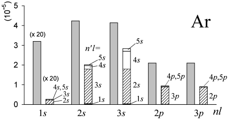
Figure 1:

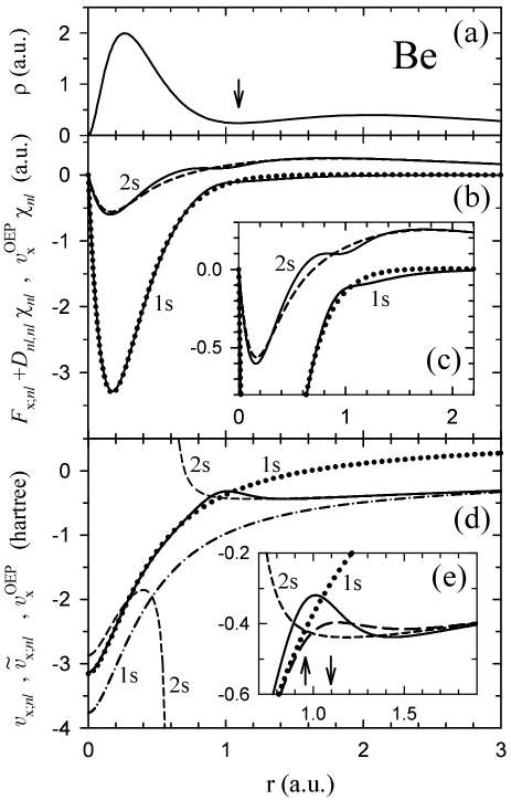
Figure 2:

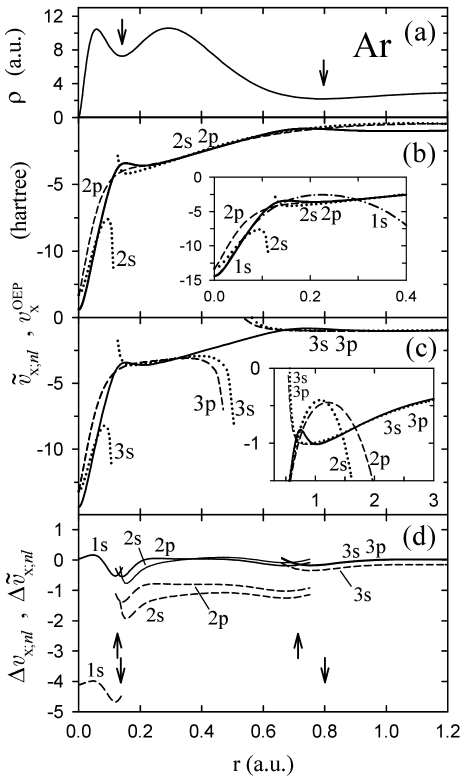
Figure 3:

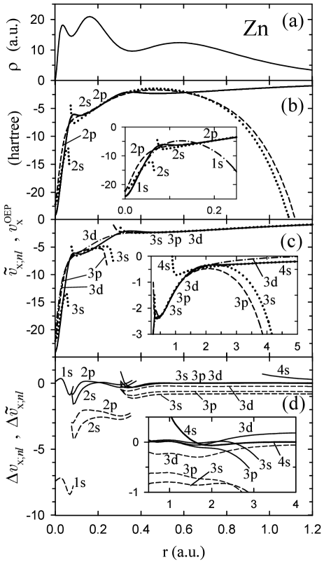
Figure 4:

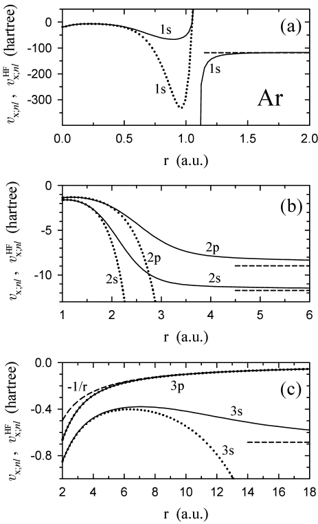
Figure 5:

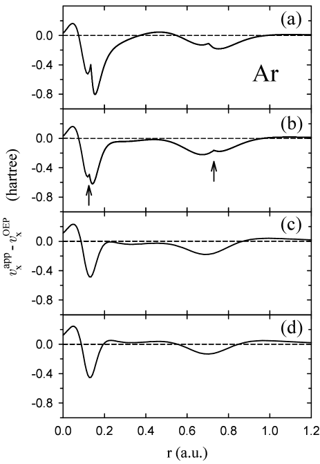
Figure 6:

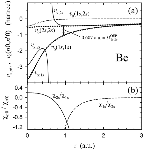
Figure 7:

References

• (1) W.R. Johnson, Atomic Structure Theory (Springer, Berlin, 2007).
• (2) R.G. Parr, W. Yang, Density-Functional Theory of Atoms and Molecules (Oxford University Press, Oxford, 1989)
• (3) R.M. Dreizler and E.K.U. Gross, Density Functional Theory: An Approach to the Quantum Many-Body Problem (Springer, Berlin,1991)).
• (4) C. Fiolhais and F. Nogueira (ed.), A Primer in Density Functional Theory, Lecture Notes in Physics 620 (Springer, Berlin, 2003).
• (5) J.B. Krieger, Y. Li, and G.J. Iafrate, Phys. Rev. A 45, 101 (1992) (a); ibid 46, 5453 (1992) (b).
• (6) E. Engel and S.H. Vosko, Phys. Rev. A 47, 2800 (1993).
• (7) T. Grabo, T. Kreibich, S. Kurth and E.K.U. Gross, Orbital functionals in density functional theory: the optimized effective potential method, in Strong Coulomb Correlations in Electronic Structure Calculations: Beyond the Local Density Approximation, ed. by V.I. Anisimov, (Gordon and Breach, 2000), p 203 - 311.
• (8) E. Engel, in Ref. FN03, , pp. 56-122.
• (9) S. KΓΌmmel and L. Kronik, Rev. Mod. Phys. 80, 3 (2008).
• (10) S. KΓΌmmel and J.P. Perdew, Phys. Rev. Lett. 90, 043004 (2003); Phys. Rev. B 68, 035103 (2003).
• (11) M. Cinal and A. Holas, Phys. Rev. A 76, 042510 (2007).
• (12) W. Yang and Q. Wu, Phys. Rev. Lett. 89, 143002 (2002).
• (13) V. N. Staroverov, G.E. Scuseria, and E.R. Davidson, J. Chem. Phys. 124, 141103 (2006).
• (14) T. Heaton-Burgess, F.A. Bulat, and W.Yang, Phys. Rev. Lett. 98, 256401 (2007).
• (15) T. Heaton-Burgess and W. Yang, J. Chem. Phys. 129, 194102 (2008).
• (16) P. BouΕ™, J. Comp. Chem., 21, 8 (2000), and the references therein.
• (17) F. Della Sala and A. GΓΆrling, J. Chem. Phys. 115, 5718 (2001).
• (18) A. GΓΆrling and M. Ernzerhof, Phys. Rev. A 51, 4501 (1995).
• (19) M. StΓ€dele, J.A. Majewski, P. Vogl, and A. GΓΆrling, Phys. Rev. Lett. 79, 2089 (1997).
• (20) M. StΓ€dele, M. Moukara, J.A. Majewski, P. Vogl, and A. GΓΆrling, Phys. Rev. B 59 , 10 031 (1999).
• (21) Q. Zhao and R.G. Parr, Phys. Rev. A 46, 2337 (1992); J. Chem. Phys. 98, 543 (1993).
• (22) Á. Nagy, J. Phys. B: At. Mol. Opt. Phys. 26, 43 (1993).
• (23) J. Chen, R. O. Esquivel, and M. J. Stott, Philos. Mag. B, 69, 1001(1994).
• (24) S. Ivanov and M. Levy, J. Chem. Phys. 119, 7087 (2003).
• (25) O. Gritsenko, R. van Leeuwen, and E.J. Baerends, Int. J. Quant. Chem. 57, 17 (1996).
• (26) O.V. Gritsenko and E.J. Baerends, Phys. Rev. A 64, 042506 (2001).
• (27) O. Gritsenko, R. van Leeuwen, and E.J. Baerends, J. Chem. Phys. 101, 8955 (1994).
• (28) R. van Leeuwen, O. Gritsenko, E.J. Baerends, Z. Phys. D. 33, 229 (1995).
• (29) The latter is not valid for $a=\text{HOMO}$, since $D_{aa}=0$, but $\Delta\epsilon_{a}=-4.13\cdot 10^{-5}\;\text{hartree}$ for Be and $-2.645\cdot 10^{-4}\;\text{hartree}$ for Ar; cf. Table 2.
• (30) C.F. Bunge, J.A. Barrientos and A.V. Bunge, Atomic Data and Nuclear Data Tables 53,113-162 (1993)
• (31) M. Cinal and A. Holas, in preparation.
• (32) F. Della Sala and A. GΓΆrling, Phys. Rev. Lett. 89, 033003 (2002).
• (33) The KS orbitals $\phi_{a}$ can be treated as the functionals of the exchange potential $v_{\text{x}}$ once they are found, in a selfconsistent way, from the KS equation with the local potential $v_{\text{s}}=v_{\text{ext}}+v_{\text{es}}[\{\phi_{a}\}]+v_{\text{x}}$. Similar functional dependence holds for a quantity, like the total energy $E$, that depends on the orbitals. The functional $E[v_{\text{x}}]=E[\{\phi_{a}[v_{\text{x}}]\}]$ is continuous because both functionals $E[\{\phi_{a}\}]$ and $\phi_{a}[v_{\text{x}}]$ ($a=1,\ldots,N$) are continuous; in the latter case the continuity is defined on the set of the physically unequivalent potentials $v_{\text{x}}$, which satisfy the condition $v_{\text{x}}(r\rightarrow\infty)=0$
• (34) M. Cinal, in preparation (2009).
• (35) N.C. Handy, M.T. Marron, and H.J. Silverstone, Phys. Rev. 180, 45 (1969).
• (36) G.S. Handler, D.W. Smith, H.J. Silverstone, J. Chem. Phys. 73, 3936 (1980).
• (37) C.L. Davis, H.-J.Aa. Jensen, H.J. Monkhorst, J. Chem. Phys. 80, 840 (1984).
• (38) T. Ishida and K.Ohno, Theor. Chim. Acta 81, 355 (1992)
• (39) A. Holas and M. Cinal, Phys. Rev. A 72, 032504 (2005).
• (40) V.N. Staroverov, G.E. Scuseria, and E.R. Davidson, J. Chem. Phys. 125, 081104 (2006).