Feynman motives and deletion-contraction relations

Abstract.

We prove a deletion-contraction formula for motivic Feynman rules given by the classes of the affine graph hypersurface complement in the Grothendieck ring of varieties. We derive explicit recursions and generating series for these motivic Feynman rules under the operation of multiplying edges in a graph and we compare it with similar formulae for the Tutte polynomial of graphs, both being specializations of the same universal recursive relation. We obtain similar recursions for graphs that are chains of polygons and for graphs obtained by replacing an edge by a chain of triangles. We show that the deletion-contraction relation can be lifted to the level of the category of mixed motives in the form of a distinguished triangle, similarly to what happens in categorifications of graph invariants.

1. Introduction

Recently, a series of results ([11], [5], [16], [8]) began to reveal the existence of a surprising connection between the world of perturbative expansions and renormalization procedures in quantum field theory and the theory of motives and periods of algebraic varieties. This lead to a growing interest in investigating algebro-geometric and motivic aspects of quantum field theory, see [2], [3], [4], [7], [12], [17], [19], [30], [31], [32], for some recent developments. Some of the main questions in the field revolve around the motivic nature of projective hypersurfaces associated to Feynman graphs. It is known by a general result of [5] that these hypersurfaces generate the Grothendieck ring of varieties, which means that, for sufficiently complicated graphs, they can become arbitrarily complex as motives. However, one would like to identify explicit conditions on the Feynman graphs that ensure that the numbers obtained by evalating the contribution of the corresponding Feynman integral can be described in algebro geometric terms as periods of a sufficiently simple form, that is, periods of mixed Tate motives. The reason to expect that this will be the case for significant classes of Feynman graphs lies in extensive databases of calculations of such integrals (see [11]) which reveal the pervasive appearance of multiple zeta values.

In [2], [3], [4] we approached the question of understanding the motivic properties of the hypersurfaces of Feynman graphs from the point of view of singularity theory. In fact, the graph hypersurfaces are typically highly singular, with singularity locus of low codimension. This has the effect that their motivic nature can often be simpler than what one would encounter in dealing with smooth hypersurfaces. This makes it possible to control the motivic complexity in terms of invariants that can measure effectively how singular the hypersurfaces are. To this purpose, in [3] we looked at algebro-geometric objects that behave like Feynman rules in quantum field theory, in the sense that they have the right type of multiplicative behavior over disjoint unions of graphs and the right type of decomposition relating one-particle-irreducible (1PI) graphs and more general connected graphs. The simplest example of such algebro-geometric Feynman rules is the affine hypersurface complement associated to a Feynman graph. This behaves like the expectation value of a quantum field theory whose edge propagator is the Tate motive ${\mathbb{Q}}(1)$. Another algebro-geometric Feynman rule we constructed in [3] is based on characteristic classes of singular varieties, assembled in the form of a polynomial $C_{\Gamma}(T)\in{\mathbb{Z}}[T]$ associated to a Feynman graph $\Gamma$.

In this paper, we investigate the dependence of these algebro-geometric Feynman rules on the underlying combinatorics of the graphs. Our approach is based on deletion–contraction relations, that is, formulae relating the invariant of a graph to that of the graphs obtained by either deleting or contracting an edge. The results we present in this paper will, in particular, answer a question on deletion–contraction relations for Feynman rules asked by Michael Falk to the first author during the Jaca conference, which motivated us to consider this problem.

It is well known that certain polynomial invariants of graphs, such as the Tutte polynomial and various invariants obtained from it by specializations, satisfy deletion–contraction relations. These are akin to the skein relations for knot and link invariants, and make it possible to compute inductively the invariant for arbitrary graphs, by progressively reducing it to simpler graphs with fewer edges.

We first show, in §2, that the Tutte polynomial and its specializations, the Tutte–Grothendieck invariants, define abstract Feynman rules in the sense of [3]. We observe that this suggests possible modifications of these invariants based on applying a Connes–Kreimer style renormalization in terms of Birkhoff factorization. This leads to modified invariants which may be worthy of consideration, although they lie beyond the purpose of this paper.

Having seen how the usual deletion–contraction relations of polynomial invariants of graphs fit in the language of Feynman rules, we consider in §3 our main object of interest, which is those abstract Feynman rules that are of algebro-geometric and motivic nature, that is, that are defined in terms of the affine graph hypersurface complement and its class in the Grothendieck ring of varieties, or its refinement introduced in [3], the ring of immersed conical varieties. We begin by showing that the polynomial invariant $C_{\Gamma}(T)$ we constructed in [3] in terms of characteristic classes is not a specialization of the Tutte polynomial, hence it is likely to be a genuinely new type of graph polynomial which may behave in a more refined way in terms of deletion and contraction. To obtain an explicit deletion–contraction relation, we consider the universal motivic Feynman rule defined by the class ${\mathbb{U}}(\Gamma)=[{\mathbb{A}}^{n}\smallsetminus\widehat{X}_{\Gamma}]$ in the Grothendieck ring of varieties of the complement of the affine graph hypersurface of a Feynman graph. Our first main result of the paper is Theorem 3.8 where we show that ${\mathbb{U}}(\Gamma)$ satisfies a deletion–contraction relation of the form

$${\mathbb{U}}(\Gamma)={\mathbb{L}}\cdot[{\mathbb{A}}^{n-1}\smallsetminus(\widehat{X}_{\Gamma\smallsetminus e}\cap\widehat{X}_{\Gamma/e})]-{\mathbb{U}}(\Gamma\smallsetminus e),$$

with ${\mathbb{L}}$ the Lefschetz motive. In §4 we reinterpret this result in terms of linear systems and Milnor fibers. This deletion–contraction formula pinpoints rather precisely the geometric mechanism by which non-mixed Tate motives will start to appear when the complexity of the graph grows sufficiently. In fact, it is the motivic nature of the intersection of the hypersurfaces $\widehat{X}_{\Gamma\smallsetminus e}\cap\widehat{X}_{\Gamma/e}$ that becomes difficult to control, even when the motives of the two hypersurfaces separately are known to be mixed Tate.

We then investigate, in §5, certain simple operations on graphs, under which one can control explicitly the effect on the motivic Feynman rule ${\mathbb{U}}(\Gamma)$ using the deletion–contraction relation. The first such example is the operation that replaces an edge in a given graph by $m$ parallel copies of the same edge. The effect on graph hypersurfaces and their classes ${\mathbb{U}}(\Gamma)$ of iterations of this operation can be packaged in the form of a generating series and a recursion, which is proved using the deletion–contraction relation. The main feature that makes it possible to control the whole recursive procedure in this case is a cancellation that eliminates the class involving the intersection of the hypersurfaces and expresses the result for arbitrary iterations as a function of just the classes ${\mathbb{U}}(\Gamma)$, ${\mathbb{U}}(\Gamma\smallsetminus e)$ and ${\mathbb{U}}(\Gamma/e)$. Our second main result in the paper is Theorem 5.3, which identifies the recursion formula and the generating function for the motivic Feynman rules under multiplication of edges in a graph.

As a comparison, we also compute explicitly in §5.1 the recusion formula satisfied by the Tutte polynomial for this same family of operations on graphs given by multiplying edges.

Another example of operations on graphs for which the resulting ${\mathbb{U}}(\Gamma)$ can be controlled in terms of the deletion–contraction relations is obtained in §5.3 by looking at graphs that are chains of polygons. This case is further reduces in §5.4 to the case of “lemon graphs” given by chains of triangles, for which an explicit recursion formula is computed. This then gives in §5.5 a similar recursion formula for the graphs obtained from a given graph by replacing a chosen edge by a lemon graph.

We then show in §6 that the recursion relations and generating functions for the motivic Feynman rule and for the Tutte polynomial under multiplication of edges in a graph are in fact closely related. We show that they are both specializations, for different choice of initial conditions, of the same universal recursion relation. We formulate a conjecture for a recursion relation for the polynomial invariant $C_{\Gamma}(T)$, based on numerical evidence collected by [33]. It again consists of a specialization of the same universal recursion relation, for yet another choice of initial conditions.

In the last section we show that one can think of the motive of the hypersurface complement in the Voevodsky triangulated category of mixed motives as a categorification of the invariant ${\mathbb{U}}(\Gamma)$, thinking of motives as a universal cohomology theory and of classes in the Grothendieck ring as a universal Euler characteristic. This categorification has properties similar to the well known categorifications of the Jones polynomial via Khovanov homology [26] and of the chromatic polynomial and the Tutte polynomial [21], [25] via versions of graph cohomology. In fact, in all of these cases the deletion–contraction relations are expressed in the categorification in the form of a long exact cohomology sequence. We show that the same happens at the motivic level, in the form of a distinguished triangle in the triangulated category of mixed motives.

2. Abstract Feynman rules and polynomial invariants

We recall briefly how the Feynman rules of a perturbative scalar field theory are defined, as a motivation for a more general notion of abstract Feynman rule, which we then describe. The reader who does not wish to see the physical motivation can skip directly to the algebraic definition of abstract Feynman rule given in Definition 2.1, and use that as the starting point. Since the main results of this paper concern certain abstract Feynman rules of combinatorial, algebro-geometric, and motivic nature, the quantum field theoretic notions we recall here serve only as background and motivation.

2.1. Feynman rules in perturbative quantum field theory

In perturbative quantum field theory, the evaluation of functional integrals computing expectation values of physical observables is obtained by expanding the integral in a perturbative series, whose terms are labeled by graphs, the Feynman graphs of the theory, whose valences at vertices are determined by the Lagrangian of the given physical theory. The number of loops of the Feynman graphs determines how far one is going into the perturbative series in order to evaluate radiative corrections to the expectation value. The contribution of individual graphs to the perturbative series is determined by the Feynman rules of the given quantum field theory. In the case of a scalar theory, these can be summarized as follows.

A graph $\Gamma$ is a Feynman graph of the theory if all vertices have valence equal to the degree of one of the monomials in the Lagrangian of the theory. Feynman graphs have internal edges, which are thought of as matching pairs of half edges connecting two of the vertices of the graph, and external edges, which are unmatched half edges connected to a single vertex. A graph is 1-particle-irreducible (1PI) if it cannot be disconnected by removal of a single (internal) edge.

We consider a scalar quantum field theory specified by a Lagrangian of the form

(2.1) $${\mathcal{L}}(\phi)=\int\left(\frac{1}{2}(\partial_{\mu}\phi)^{2}+\frac{m^{2}}{2}\phi^{2}+{\mathcal{P}}(\phi)\right)dv,$$

where we use Euclidean signature in the metric on the underlying spacetime ${\mathbb{R}}^{D}$ and the interaction term is a polynomial of the form

(2.2) $${\mathcal{P}}(\phi)=\sum_{k}\frac{\lambda_{k}}{k!}\phi^{k}.$$

In the following we will treat the dimension $D$ of the underlying spacetime as a variable parameter.

To a connected Feynman graph of a given scalar quantum field theory one assigns a function $V(\Gamma,p_{1},\ldots,p_{N})$ of the external momenta in the following way.

Each internal edge $e\in E_{int}(\Gamma)$ contributes a momentum variable $k_{e}\in{\mathbb{R}}^{D}$ and the function of the external momenta is obtained by integrating a certain density function over the momentum variables of the internal edges,

(2.3) $$V(\Gamma,p_{1},\ldots,p_{N})=\int{\mathcal{I}}_{\Gamma}(p_{1},\ldots,p_{N},k_{1},\ldots,k_{n})\frac{d^{D}k_{1}}{(2\pi)^{D}}\cdots\frac{d^{D}k_{n}}{(2\pi)^{D}},$$

for $n=\#E_{int}(\Gamma)$. We write $k=(k_{e})$ for the collection of all the momentum variables assigned to the internal edges.

The term ${\mathcal{I}}_{\Gamma}(p_{1},\ldots,p_{N},k_{1},\ldots,k_{n})$ is constructed according to the following procedure. Each vertex $v\in V(\Gamma)$ contributes a factor of $\lambda_{v}(2\pi)^{D}$, where $\lambda_{v}$ is the coupling constant of the monomial in the interaction term (2.2) in the Lagrangian of order equal to the valence of $v$. One also imposes a conservation law on the momenta that flow through a vertex,

(2.4) $$\delta_{v}(k):=\delta(\sum_{s(e)=v}k_{e}-\sum_{t(e)=v}k_{e}),$$

written after chosing an orientation of the edges of the graph, so that $s(e)$ and $t(e)$ are the source and target of an edge $e$. When a vertex is attached to both internal and external edges, the conservation law (2.4) at that vertex will be of an analogous form $\delta_{v}(k,p)$, involving both the $k$ variables of the momenta along internal edges and the $p$ variables of the external momenta. We will see later that the dependence on the choice of the orientation disappears in the final form of the Feynman integral.

Each internal edge $e\in E_{int}(\Gamma)$ contributes an inverse propagator, that is, a term of the form $q_{e}^{-1}$, where $q_{e}$ is a quadratic form, which in the case of a scalar field in the Euclidean signature is given by

(2.5) $$q_{e}(k_{e})=k_{e}^{2}+m^{2}.$$

Each external edge $e\in E_{ext}(\Gamma)$ contributes an inverse propagator $q_{e}(p_{e})^{-1}$, with $q_{e}(p_{e})=p_{e}^{2}+m^{2}$. The external momenta are assigned so that they satisfy the conservation law $\sum_{e}p_{e}=0$, when summed over the oriented external edges.

The integrand ${\mathcal{I}}_{\Gamma}(p_{1},\ldots,p_{N},k_{1},\ldots,k_{n})$ is then a product

(2.6) $$\prod_{v\in V(\Gamma)}\lambda_{v}(2\pi)^{D}\,\,\delta_{v}(k,p)\,\,\prod_{e\in E_{int}(\Gamma)}q_{e}(k_{e})^{-1}\prod_{e\in E_{ext}(\Gamma)}q_{e}(p_{e})^{-1}.$$

The Feynman rules defined in this way satisfy two main properties, which follow easily from the construction described above (see [29], [32]).

The Feynman rules are multiplicative over disjoint unions of graphs (hence one can reduce to considering only connected graphs):

(2.7) $$V(\Gamma,p_{1},\ldots,p_{N_{1}},p_{1}^{\prime},\ldots,p_{N_{2}}^{\prime})=V(\Gamma_{1},p_{1},\ldots,p_{N_{1}})V(\Gamma_{2},p_{1}^{\prime},\ldots,p_{N_{2}}^{\prime}),$$

for a disjoint union $\Gamma=\Gamma_{1}\cup\Gamma_{2}$, of two Feynman graphs $\Gamma_{1}$ and $\Gamma_{2}$, with external momenta $p=(p_{1},\ldots,p_{N_{1}})$ and $p^{\prime}=(p_{1}^{\prime},\ldots,p_{N_{2}}^{\prime})$, respectively.

Any connected graph $\Gamma$ can be obtained from a finite tree $T$ by replacing vertices $v$ of $T$ with 1PI graphs $\Gamma_{v}$ with number of external edges equal to the valence of the vertex $v$. Then the Feynman rules satisfy

(2.8) $$V(\Gamma,p)=\prod_{v\in V(T),e\in E_{int}(T),v\in\partial(e)}V(\Gamma_{v},p_{v})\,\,q_{e}(p_{v})^{-1}\,\,\delta((p_{v})_{e}-(p_{v^{\prime}})_{e}).$$

The delta function in this expression matches the external momenta of the 1PI graphs inserted at vertices sharing a common edge.

Up to a factor containing the inverse propagators of the external edges and the coupling constants of the vertices, we write

$$V(\Gamma,p_{1},\ldots,p_{N})=C\varepsilon(p_{1},\ldots,p_{N})\,U(\Gamma,p_{1},\ldots,p_{N}),$$

with $C=\prod_{v\in V(\Gamma)}\lambda_{v}(2\pi)^{D}$ and $\varepsilon(p_{1},\ldots,p_{N})=\prod_{e\in E_{ext}(\Gamma)}q_{e}(p_{e})^{-1}$ and the remaining term is

(2.9) $$U(\Gamma,p_{1},\ldots,p_{N})=\frac{\delta(\sum_{i=1}^{n}\epsilon_{v,i}k_{i}+\sum_{j=1}^{N}\epsilon_{v,j}p_{j})}{q_{1}(k_{1})\cdots q_{n}(k_{n})},$$

where we have written the delta functions $\delta_{v}(k,p)$ of (2.4) equivalently in terms of the edge-vertex incidence matrix of the graph, $\epsilon_{v,i}=\pm 1$ when $v=t(e)$ or $v=s(e)$ and $\epsilon_{v,i}=0$ otherwise. The Feynman integrals (2.9) still satisfy the two properties (2.7) and (2.8).

Notice that the property (2.8) expressing the Feynman rule for connected graphs in terms of Feynman rules for 1PI graphs has a simpler form in the case where either all external momenta are set equal to zero and the theory is massive ($m\neq 0$), or all external momenta are equal. In such cases (2.8) reduces to a product

$$U(\Gamma,p)=U(L)^{\#E_{int}(T)}\prod_{v\in V(T)}U(\Gamma_{v},p_{v}),$$

with $U(L)$ the inverse propagator assigned to a single edge.

2.2. Abstract Feynman rules

In [3] we abstracted the two properties of Feynman rules recalled above and used them to define a class of algebro-geometric Feynman rules.

More precisely, we defined an abstract Feynman rule in the following way.

Definition 2.1.

An abstract Feynman rule is a map from the set of (isomorphism classes of) finite graphs to a commutative ring ${\mathcal{R}}$, with the property that it is multiplicative over disjoint unions of graphs,

(2.10) $$U(\Gamma_{1}\cup\Gamma_{2})=U(\Gamma_{1})U(\Gamma_{2}),$$

and such that, for a connected graph $\Gamma=\cup_{v\in V(T)}\Gamma_{v}$ obtained by inserting 1PI graphs $\Gamma_{v}$ at the vertices of a tree $T$, it satisfies

(2.11) $$U(\Gamma)=U(L)^{\#E_{int}(T)}\prod_{v\in V(T)}U(\Gamma_{v}),$$

where $U(L)$ is the inverse propagator, that is, the value assigned to the graph consiting of a single edge.

The multiplicative property with respect to disjoint unions of graphs, together with the second property which implies that 1PI graphs are sufficient to determine completely the Feynmal rule, means that an abstract Feynman rule with values in ${\mathcal{R}}$ can be reformulated as a ring homomorphism from a Hopf algebra ${\mathcal{H}}$ of Feynman graphs to ${\mathcal{R}}$. In this general setting, since we are not choosing a particular Lagrangian of the theory, the Hopf algebra is not the usual Connes–Kreimer Hopf algebra [14], which depends on the Lagrangian of a particular theory but the larger Hopf algebra referred to in [9] and [27] as the “core Hopf algebra”. As an algebra (or a ring) this is a polynomial algebra generated by all 1PI graphs and the coproduct is of the form

(2.12) $$\Delta(\Gamma)=\Gamma\otimes 1+1\otimes\Gamma+\sum_{\gamma\subset\Gamma}\gamma\otimes\Gamma/\gamma,$$

where the sum is over subgraphs whose connected components are 1PI. The quotient $\Gamma/\gamma$ is obtained by shrinking each component of $\gamma$ to a single vertex. The Hopf algebra is graded by loop number (or by number of internal edges) and the antipode is defined inductively by

$$S(\Gamma)=-\Gamma-\sum S(\gamma)\,\Gamma/\gamma.$$

Notice that the multiplicative property of Feynman rules only relates to the algebra, not the coalgebra, structure of the Hopf algebra of Feynman graphs. Where the coproduct and the antipode enter essentially is in the renormalization of abstract Feynman rules, which can again be formulated purely algebraically in terms of a Rota–Baxter structure of weight $-1$ on the target ring ${\mathcal{R}}$ (see [15], [20]).

We now show that the notion of abstract Feynman rule is very natural. In fact, a broad range of classical combinatorial invariants of graphs define abstract Feynman rules.

2.3. Tutte–Grothendieck polynomials as a Feynman rules

For a finite graph $\Gamma$, one denotes by $\Gamma\smallsetminus e$ the graph obtained by deleting an edge $e\in E(\Gamma)$ and by $\Gamma/e$ the graph obtained by contracting an edge $e\in E(\Gamma)$ to a vertex. They are called, respectively, the deletion and contraction of $\Gamma$ at $e$. A class of invariants of graphs that behave well with respect to the operations of deletion and contraction are known as the Tutte–Grothendieck invariants [10], [13], [18]. The terminology comes from the Tutte polynomial, which is the prototype example of such invariants, and from the formulation in terms of Grothendieck rings of certain categories, as in [13].

Tutte–Grothendieck invariants of graphs are defined as functions $F(\Gamma)$ from the set of (isomorphism classes of) finite graphs to a polynomial ring ${\mathbb{C}}[\alpha,\beta,\gamma,x,y]$ which satisfy the following properties.

• $F(\Gamma)=\gamma^{\#V(\Gamma)}$ if the set of edges is empty, $E(\Gamma)=\emptyset$.

• $F(\Gamma)=xF(\Gamma\smallsetminus e)$ if the edge $e\in E(\Gamma)$ is a bridge.

• $F(\Gamma)=yF(\Gamma/e)$ if $e\in E(\Gamma)$ is a looping edge.

• For $e\in E(\Gamma)$ not a bridge nor a looping edge,

  (2.13) $$F(\Gamma)=\alpha F(\Gamma/e)+\beta F(\Gamma\smallsetminus e).$$

Recall that an edge is a bridge (or isthmus) if the removal of $e$ disconnects the graph $\Gamma$. A looping edge is an edge that starts and ends at the same vertex. The relation (2.13) is the deletion–contraction relation. By repeatedly applying it until one falls into one of the other case, this makes it possible to completely determine the value of a Tutte–Grothendieck invariant for all graphs.

Tutte–Grothendieck invariants are specializations of the Tutte polynomial. The latter is defined by the properties that

(2.14) $${\mathcal{T}}_{\Gamma}(x,y)=x^{i}y^{j},$$

if the graph $\Gamma$ consists of $i$ bridges, $j$ looping edges and no other edges, and by the deletion–contraction relation

(2.15) $${\mathcal{T}}_{\Gamma}(x,y)={\mathcal{T}}_{\Gamma\smallsetminus e}(x,y)+{\mathcal{T}}_{\Gamma/e}(x,y).$$

Clearly the relation (2.15) together with (2.14) determine the Tutte polynomial for all graphs. The closed formula is given by the “sum over states” formula

(2.16) $${\mathcal{T}}_{\Gamma}(x,y)=\sum_{\gamma\subset\Gamma}(x-1)^{\#V(\Gamma)-b_{0}(\Gamma)-(\#V(\gamma)-b_{0}(\gamma))}(y-1)^{\#E(\gamma)-\#V(\gamma)+b_{0}(\gamma)},$$

where the sum is over subgraphs $\gamma\subset\Gamma$ with vertex set $V(\gamma)=V(\Gamma)$ and edge set $E(\gamma)\subset E(\Gamma)$. This can be written equivalently as

$${\mathcal{T}}_{\Gamma}(x,y)=\sum_{\gamma\subset\Gamma}(x-1)^{b_{0}(\gamma)-b_{0}(\Gamma)}(y-1)^{b_{1}(\gamma)}.$$

An equivalent way to express the recursive relations computing the Tutte polynomials is the following:

• If $e\in E(\Gamma)$ is neither a looping edge nor a bridge the deletion–contraction relation (2.15) holds.

• If $e\in E(\Gamma)$ is a looping edge then

  $${\mathcal{T}}_{\Gamma}(x,y)=y{\mathcal{T}}_{\Gamma/e}(x,y).$$

• If $e\in E(\Gamma)$ is a bridge then

  $${\mathcal{T}}_{\Gamma}(x,y)=x{\mathcal{T}}_{\Gamma\smallsetminus e}(x,y)$$

• If $\Gamma$ has no edges then $T_{\Gamma}(x,y)=1$.

A Tutte–Grothendieck invariant satisfying (2.13) is then obtained from the Tutte polynomial by specialization

(2.17) $$F(\Gamma)=\gamma^{b_{0}(\Gamma)}\alpha^{\#V(\Gamma)-b_{0}(\Gamma)}\beta^{b_{1}(\Gamma)}\,{\mathcal{T}}_{\Gamma}(\frac{\gamma x}{\alpha},\frac{y}{\beta}).$$

Among the invariants that can be obtained as specializations of the Tutte polynomial are the chromatic polynomial of graphs and the Jones polynomial of links, viewed as an invariant of an associated planar graph, [34], [24].

The chromatic polynomial $P(\Gamma,\lambda)$ is a specialization of the Tutte polynomial through

(2.18) $$P(\Gamma,\lambda)=(-1)^{\#V(\Gamma)-b_{0}(\Gamma)}\lambda^{b_{0}(\Gamma)}{\mathcal{T}}_{\Gamma}(1-\lambda,0).$$

In the case of an alternating link $L$, the Jones polynomial is a specialization of the associated (positive) checkerboard graph $\Gamma_{+}$ by

$$J(L,t)=(-1)^{w}t^{(\#V(\Gamma_{-})-\#V(\Gamma_{+})+3w)/4}\,\,{\mathcal{T}}_{\Gamma_{+}}(-t,-1/t),$$

with $w$ the writhe (algebraic crossing number) and $\Gamma_{\pm}$ the positive and negative checkerboard graphs associated to $L$, [10].

Proposition 2.2.

The Tutte polynomial invariant defines an abstract Feynman rule with values in the polynomial ring ${\mathbb{C}}[x,y]$, by assigning

(2.19) $$U(\Gamma)={\mathcal{T}}_{\Gamma}(x,y),\ \ \ \text{ with inverse propagator }\ \ \ U(L)=x.$$

Similarly, any Tutte–Grothendieck invariant determines an abstract Feynman rule with values in ${\mathbb{C}}[\alpha,\beta,\gamma,x,y]$ by assigning $U(\Gamma)=F(\Gamma)$ with inverse propagator $U(L)=x$.

Proof.

It suffices to check that the Tutte polynomial is multiplicative over disjoint unions of graphs and that, under the decomposition of connected graphs into a tree with 1PI graphs inserted at the vertices, it satisfies the property (2.11). The multiplicative property is clear from the closed expression (2.16), since for $\Gamma=\Gamma_{1}\cup\Gamma_{2}$ we can identify subgraphs $\gamma\subset\Gamma$ with $V(\gamma)=V(\Gamma)$ and $E(\gamma)\subset E(\Gamma)$ with all possible pairs of subgraphs $(\gamma_{1},\gamma_{2})$ with $V(\gamma_{i})=V(\Gamma_{i})$ and $E(\gamma_{i})\subset E(\Gamma_{i})$, with $b_{0}(\gamma)=b_{0}(\gamma_{1})+b_{0}(\gamma_{2})$, $\#V(\Gamma)=\#V(\Gamma_{1})+\#V(\Gamma_{2})$, and $\#E(\gamma)=\#E(\gamma_{1})+\#E(\gamma_{2})$. Thus, we get

$$\begin{array}[]{rl}{\mathcal{T}}_{\Gamma}(x,y)=&\sum_{\gamma=(\gamma_{1},\gamma_{2})}(x-1)^{b_{0}(\gamma_{1})+b_{0}(\gamma_{2})-b_{0}(\Gamma)}(y-1)^{b_{1}(\gamma_{1})+b_{1}(\gamma_{2})}\\[5.69054pt] =&{\mathcal{T}}_{\Gamma_{1}}(x,y)\,{\mathcal{T}}_{\Gamma_{2}}(x,y).\end{array}$$

The second property for connected and 1PI graphs follows from the fact that, when writing a connected graph in the form $\Gamma=\cup_{v\in V(T)}\Gamma_{v}$, with $\Gamma_{v}$ 1PI graphs inserted at the vertices of the tree $T$, the internal edges of the tree are all bridges in the resulting graph, hence the property of the Tutte polynomial for the removal of bridges gives

$${\mathcal{T}}_{\Gamma}(x,y)=x^{\#E_{int}(T)}\,\,{\mathcal{T}}_{\Gamma\smallsetminus\cup_{e\in E_{int}(T)}e}(x,y).$$

Then one obtains an abstract Feynman rule with values in ${\mathcal{R}}={\mathbb{C}}[x,y]$ of the form (2.19).

In fact, the multiplicative property follows from the same property for the Tutte polynomial and the specialization formula (2.17). The case of connected and 1PI graphs again follow from the property of Tutte–Grothendieck invariants that $F(\Gamma)=xF(\Gamma\smallsetminus e)$, when $e\in E(\Gamma)$ is a bridge, exactly in the same way as in the case of ${\mathcal{T}}_{\Gamma}(x,y)$. ∎

This implies that both the chromatic and the Jones polynomial, for instance, can be regarded as abstract Feynman rules.

As we have mentioned above, whenever the ring ${\mathcal{R}}$ where an abstract Feynman rule takes values has the structure of a Rota–Baxter algebra of weight $-1$, the Feynman rule can be renormalized. This works in the following way.

A Rota–Baxter operator of weight $\lambda$ is a linear operator ${\mathfrak{T}}:{\mathcal{R}}\to{\mathcal{R}}$ satisfying

(2.20) $${\mathfrak{T}}(x){\mathfrak{T}}(y)={\mathfrak{T}}(x{\mathfrak{T}}(y))+{\mathfrak{T}}({\mathfrak{T}}(x)y)+\lambda{\mathfrak{T}}(xy).$$

In the case where $\lambda=-1$, such an operator determines a decomposition of the ring ${\mathcal{R}}$ into two commutative unital rings ${\mathcal{R}}_{\pm}$ defined by ${\mathcal{R}}_{+}=(1-{\mathfrak{T}}){\mathcal{R}}$ and ${\mathcal{R}}_{-}$ the ring obtained by adjoining a unit to the nonunital ${\mathfrak{T}}{\mathcal{R}}$. An example of $({\mathcal{R}},{\mathfrak{T}})$ is given by Laurent series with the projection onto the polar part.

The Connes–Kreimer interpretation [14] [15] of the BPHZ renormalization procedure as a Birkhoff factorization of loops with values in the affine group scheme dual to the Hopf algebra of Feynman graphs can be formulated equivalently in terms of the Rota–Baxter structure [20]. The Connes–Kreimer recursive formula for the Birkhoff factorization of an algebra homomorphism $U:{\mathcal{H}}\to{\mathcal{R}}$ is given as in [14] by

(2.21) $$\begin{array}[]{rl}U_{-}(\Gamma)=&-\displaystyle{{\mathfrak{T}}\left(U(\Gamma)+\sum_{\gamma\subset\Gamma}U_{-}(\gamma)U(\Gamma/\gamma)\right)}\\[8.53581pt] U_{+}(\Gamma)=&\displaystyle{(1-{\mathfrak{T}})\left(U(\Gamma)+\sum_{\gamma\subset\Gamma}U_{-}(\gamma)U(\Gamma/\gamma)\right)}.\end{array}$$

Of these, the $U_{-}$ term gives the counterterms and the $U_{+}$ gives the renormalized value.

Thus, for example, when one considers specializations of the Tutte polynomial such as the Jones polynomial, which take values in a ring of Laurent series, one can introduce a renormalized version of the invariant obtained by performing the Birkhoff factorization of the corresponding character of the Hopf algebra of Feynman graphs. It would be interesting to see if properties of the coefficients of the Jones polynomial, such as the fact that they are not finite type invariants, may be affected by this renormalization procedure.

3. Graph hypersurfaces and deletion-contraction relations

In [3] we considered in particular abstract Feynman rules that are algebro-geometric or motivic, which means that they factor through the information on the affine hypersurface defined by the Kirchhoff polynomial of the graph, which appears in the parametric form of Feynman integrals. We recall here how the graph hypersurfaces are defined and how they arise in the original context of parametric Feynman integrals. We recall from [3] how one can use the affine hypersurface complement to define algebro-geometric and motivic Feynman rules, and we then prove that motivic Feynman rules satisfy a more complicated variant of the deletion–contraction relation discussed above.

3.1. Parametric Feynman integrals and graph hypersurfaces

The Feynman rules (2.9) for a scalar quantum field theory can be reformulated in terms of Feynman parameters (see [6], [23]) in the form of an integral of an algebraic differential form on a cycle with boundary in the complement of a hypersurface defined by the vanishing of the graph polynomial. The parametric form of the Feynman integral, in the massless case $m=0$, is given by

(3.1) $$U(\Gamma,p_{1},\ldots,p_{N})=\frac{\Gamma(n-\frac{D\ell}{2})}{(4\pi)^{D\ell/2}}\int_{\sigma_{n}}\frac{P_{\Gamma}(t,p)^{-n+D\ell/2}\omega_{n}}{\Psi_{\Gamma}(t)^{-n+D(\ell+1)/2}},$$

where $n=\#E_{int}(\Gamma)$ and $\ell=b_{1}(\Gamma)$. The domain of integration is the simplex $\sigma_{n}=\{t\in{\mathbb{R}}_{+}^{n}\,|\,\sum_{i}t_{i}=1\}$. The Kirchhoff–Symanzik polynomial $\Psi_{\Gamma}(t)$ is given by

(3.2) $$\Psi_{\Gamma}(t)=\sum_{T\subset\Gamma}\prod_{e\notin E(T)}t_{e},$$

where the sum is over all the spanning forests $T$ (spanning trees in the connected case) of the graph $\Gamma$ and for each spanning forest the product is over all edges of $\Gamma$ that are not in that spanning forest. The polynomial $P_{\Gamma}(t,p)$, often referred to as the second Symanzik polynomial, is similarly defined in terms of the combinatorics of the graph, using cut sets instead of spanning trees, and it depends explicitly on the external momenta of the graph (see [6] §18). In the following, we assume for simplicity to work in the “stable range” where $-n+D\ell/2>0$. In this case, further assuming that for general choice of the external momenta the polynomials $\Psi_{\Gamma}(t)$ and $P_{\Gamma}(t,p)$ do not have common factors, the parametric Feynman integral (3.1) is defined in the complement of the hypersurface

(3.3) $$\widehat{X}_{\Gamma}=\{t\in{\mathbb{A}}^{n}\,|\,\Psi_{\Gamma}(t)=0\}.$$

Since $\Psi_{\Gamma}$ is homogeneous of degree $\ell$, one can reformulate the period computation in projective space in terms of the hypersurface

$$X_{\Gamma}=\{t\in{\mathbb{P}}^{n-1}\,|\,\Psi_{\Gamma}(t)=0\},$$

see [8]. Up to a divergent Gamma-factor, one is then interested in understanding the nature of the remaining integral (the residue of the Feynman graph)

(3.4) $$\int_{\sigma_{n}}\frac{P_{\Gamma}(t,p)^{-n+D\ell/2}\omega_{n}}{\Psi_{\Gamma}(t)^{-n+D(\ell+1)/2}}.$$

viewed (possibly after eliminating divergences) as a period of an algebraic variety. The complexity of the period depends on the motivic complexity of the part of the cohomology of the algebraic variety that is involved in the period evaluation. In this case, the integration is on the domain $\sigma_{n}$ with boundary $\partial\sigma_{n}\subset\widehat{\Sigma}_{n}$ contained in the divisor $\widehat{\Sigma}_{n}\subset{\mathbb{A}}^{n}$ given by the union of coordinate hyperplanes $\widehat{\Sigma}_{n}=\{t\in{\mathbb{A}}^{n}\,|\,\prod_{i}t_{i}=0\}$, hence the relative cohomology involved in the period computation is

(3.5) $$H^{n-1}({\mathbb{P}}^{n-1}\smallsetminus X_{\Gamma},\Sigma_{n}\smallsetminus(X_{\Gamma}\cap\Sigma_{n})),$$

where $\Sigma_{n}$ is the divisor of coordinate hyperplanes in ${\mathbb{P}}^{n-1}$. The main question one would like to address is under what conditions on the graph this cohomology is a realization of a mixed Tate motive, which in turn gives a strong bound on the complexity of the periods.

A way to understand the motivic complexity of (3.5) is to look at classes in the Grothendieck ring of varieties. A result of Belkale–Brosnan [5] shows that the classes $[X_{\Gamma}]$ of the graph hypersurfaces generate the Grothendieck ring, so they can be arbitrarily complex as motives and not only of mixed Tate type. It is still possible, however, that the piece of the cohomology involved in (3.4) may still be mixed Tate even if $X_{\Gamma}$ itself contains non-mixed Tate strata.

3.2. Algebro-geometric and motivic Feynman rules

Coming back to abstract Feynman rules, we observed in [3] that the affine hypersurface complement ${\mathbb{A}}^{n}\smallsetminus\widehat{X}_{\Gamma}$ behaves like a Feynman rule, in the sense that it satisfies the multiplicative property under disjoint unions of graphs

(3.6) $${\mathbb{A}}^{n}\smallsetminus\widehat{X}_{\Gamma}=({\mathbb{A}}^{n_{1}}\smallsetminus\widehat{X}_{\Gamma_{1}})\times({\mathbb{A}}^{n_{2}}\smallsetminus\widehat{X}_{\Gamma_{2}}),$$

for $\Gamma=\Gamma_{1}\cup\Gamma_{2}$ a disjoint union. The role of the inverse propagator is played by the affine line ${\mathbb{A}}^{1}$.

We introduced in [3] a Grothendieck ring of immersed conical varieties ${\mathcal{F}}$ which is generated by the equivalence classes $[\widehat{X}]$ up to linear changes of coordinates of varieties $\widehat{X}\subset{\mathbb{A}}^{N}$ embedded in some affine space, that are defined by homogeneous ideals (affine cones over projective varieties), with the usual inclusion–exclusion relation

$$[\widehat{X}]=[\widehat{Y}]+[\widehat{X}\smallsetminus\widehat{Y}]$$

for $\widehat{Y}\subset\widehat{X}$ a closed embedding. This maps to the usual Grothendieck ring of varieties $K_{0}({\mathcal{V}})$ by passing to isomorphisms classes of varieties.

We then defined in [3] algebro-geometric and motivic Feynman rules in the following way.

Definition 3.1.

An algebro geometric Feynman rule is an abstract Feynman rule $U:{\mathcal{H}}\to{\mathcal{R}}$, which factors through the Grothendieck ring of immersed conical varieties,

(3.7) $$U(\Gamma)=I([{\mathbb{A}}^{n}\smallsetminus\widehat{X}_{\Gamma}]),$$

where $[{\mathbb{A}}^{n}\smallsetminus\widehat{X}_{\Gamma}]$ is the class in ${\mathcal{F}}$ of the affine graph hypersurface complement and $I:{\mathcal{F}}\to{\mathcal{R}}$ is a ring homomorphism. A motivic Feynman rule is an abstract Feynman rule that similarly factors through the Grothendieck ring of varieties as in (3.7) with $[{\mathbb{A}}^{n}\smallsetminus\widehat{X}_{\Gamma}]$ the class in $K_{0}({\mathcal{V}})$ and a ring homomorphism $I:K_{0}({\mathcal{V}})\to{\mathcal{R}}$.

It is then natural to ask whether these abstract Feynman rules, like the examples of abstract Feynman rules we have described in §2.3 above, satisfy deletion–contraction relations. We show in §3.4 below that there is a deletion–contraction relation for the graph hypersurfaces and their classes in the Grothendieck ring, which is, however, of a more subtle form than the one satisfied by Tutte–Grothendieck invariants. We first show that the polynomial invariant of graphs we introduced in [3] as an example of an algebro-geometric Feynman rule which is not motivic (it does not factor through the Grothendieck ring) is not a specialization of the Tutte polynomial.

3.3. The Chern–Schwartz–MacPherson Feynman rule

In particular, we constructed in [3] an algebro-geometric Feynman rule given by a polynomial invariant $C_{\Gamma}(T)$ constructed using Chern–Schwartz–MacPherson characteristic classes of singular varieties. Without going into the details of the definition and properties of this invariant, for which we refer the reader to [3], we just mention briefly how it is obtained. One obtains a ring homomorphism $I_{CSM}:{\mathcal{F}}\to{\mathbb{Z}}[T]$ from the ring of immersed conical varieties to a polynomial ring by assigning to the class $[\widehat{X}]$ of a variety in ${\mathcal{F}}$ the polynomial

$$I_{CSM}([\widehat{X}])=a_{0}+a_{1}T+\cdots a_{N}T^{N}$$

where $\widehat{X}\subset{\mathbb{A}}^{N}$ (viewed as a locally closed subscheme of ${\mathbb{P}}^{N}$) has Chern–Schwartz–MacPherson (CSM) class

$$c_{*}(1_{\widehat{X}})=a_{0}[{\mathbb{P}}^{0}]+a_{1}[{\mathbb{P}}^{1}]+\cdots a_{N}[{\mathbb{P}}^{N}]$$

in the Chow group (or homology) of ${\mathbb{P}}^{N}$. It is shown in [3] that this is well defined and is indeed a ring homomorphism, which involves some careful analysis of the behavior of CSM classes for joins of projective varieties. One then defines the polynomial invariant of graphs as

$$C_{\Gamma}(T)=I_{CSM}([{\mathbb{A}}^{n}\smallsetminus\widehat{X}_{\Gamma}]).$$

It is natural to ask whether this polynomial invariant may be a specialization of the Tutte polynomial. We show in the remaining of this section that this is not the case: the invariant $C_{\Gamma}(T)$ is not a specialization of the Tutte polynomial, hence it appears to be a genuinely new invariant of graphs.

Proposition 3.2.

The polynomial invariant $C_{\Gamma}(T)$ is not a specialization of the Tutte polynomial.

Proof.

We show that one cannot find functions $x=x(T)$ and $y=y(T)$ such that

$$C_{\Gamma}(T)={\mathcal{T}}_{\Gamma}(x(T),y(T)).$$

First notice that, if $e\in E(\Gamma)$ is a bridge, the polynomial $C_{\Gamma}(T)$ satisfies the relation

(3.8) $$C_{\Gamma}(T)=(T+1)C_{\Gamma\smallsetminus e}(T).$$

In fact, $(T+1)$ is the inverse propagator of the algebro-geometric Feynman rule $U(\Gamma)=C_{\Gamma}(T)$ and the property of abstract Feynman rules for 1PI graphs connected by a bridge gives (3.8). In the case where $e\in E(\Gamma)$ is a looping edge, we have

(3.9) $$C_{\Gamma}(T)=T\,\,C_{\Gamma/e}(T).$$

In fact, adding a looping edge to a graph corresponds, in terms of graph hypersurfaces, to taking a cone on the graph hypersurface and intersecting it with the hyperplane defined by the coordinate of the looping edge. This implies that the universal algebro-geometric Feynman rule with values in the Grothendieck ring ${\mathcal{F}}$ of immersed conical varieties satisfies

$${\mathbb{U}}(\Gamma)=([{\mathbb{A}}^{1}]-1){\mathbb{U}}(\Gamma/e)$$

if $e$ is a looping edge of $\Gamma$ and ${\mathbb{U}}(\Gamma)=[{\mathbb{A}}^{n}\smallsetminus\widehat{X}_{\Gamma}]\in{\mathcal{F}}$. The property (3.9) then follows since the image of the class $[{\mathbb{A}}^{1}]$ is the inverse propagator $(T+1)$. (See Proposition 2.5 and §2.2 of [3].)

This implies that, if $C_{\Gamma}(T)$ has to be a specialization of the Tutte polynomial, the relations for bridges and looping edges imply that one has to identify $x(T)=T+1$ and $y(T)=T$. However, this is not compatible with the behavior of the invariant $C_{\Gamma}(T)$ on more complicated graphs. For example, for the triangle graph one has $C_{\Gamma}(T)=T(T+1)^{2}$ while the specialization ${\mathcal{T}}_{\Gamma}(x(T),y(T))=(T+1)^{2}+(T+1)+T$. ∎

The reason for this discrepancy is the fact that, while any algebro-geometric or motivic Feynman rule will have the same behavior as the Tutte polynomial for looping edges and bridges, the more general deletion–contraction relation does not hold. The class $[{\mathbb{A}}^{n}\smallsetminus\widehat{X}_{\Gamma}]$ in the Grothendieck ring of varieties $K_{0}({\mathcal{V}})$ satisfies a more subtle deletion–contraction relation, which we now describe.

3.4. Deletion–contraction for motivic Feynman rules

We begin by considering a more general situation, which we then specialize to the case of the graph hypersurfaces. In this general setting, we consider two homogeneous polynomials $F$ and $G$ of degree $\ell-1$ and $\ell$, respectively, in variables $t_{1},\dots,t_{n-1}$, with $n\geq 2$. Let

(3.10) $$\psi(t_{1},\ldots,t_{n})=t_{n}F(t_{1},\dots,t_{n-1})+G(t_{1},\dots,t_{n-1}).$$

Thus, $\psi$ is homogeneous of degree $\ell$ in $t_{1},\dots,t_{n}$. Assume that both $F$ and $G$ and not identically zero, so that it makes sense to consider the hypersurfaces defined by these polynomials. Cases where either $F$ or $G$ are zero are easily analyzed separately. We denote then by $X$ and $Y$ the projective hypersurfaces in ${\mathbb{P}}^{n-1}$ and ${\mathbb{P}}^{n-2}$, respectively, determined by $\psi$ and $F$. We denote by $\overline{Y}$ the cone of $Y$ in ${\mathbb{P}}^{n-1}$, that is, the hypersurface defined in ${\mathbb{P}}^{n-1}$ by the same polynomial $F$.

Theorem 3.3.

With notation as above, the projection from the point $(0:\dots:0:1)$ induces an isomorphism

(3.11) $$X\smallsetminus(X\cap\overline{Y})\overset{\sim}{\longrightarrow}{\mathbb{P}}^{n-2}\smallsetminus Y.$$

Proof.

The projection ${\mathbb{P}}^{n-1}\dashrightarrow{\mathbb{P}}^{n-2}$ from $p=(0:\dots:0:1)$ acts as

$$(t_{1}:\dots:t_{n})\mapsto(t_{1}:\dots:t_{n-1}).$$

If $F$ is constant (that is, if $\deg\psi=1$), then $Y=\overline{Y}=\emptyset$ and the statement is trivial. Thus, assume $\deg F>0$. In this case, $\psi(p)=F(p)=0$, hence $p\in X\cap\overline{Y}$, and hence $p\not\in X\smallsetminus(X\cap\overline{Y})$. Therefore, the projection restricts to a regular map

$$X\smallsetminus(X\cap\overline{Y})\to{\mathbb{P}}^{n-2}.$$

The image is clearly contained in ${\mathbb{P}}^{n-2}\smallsetminus Y$, and the statement is that this map induces an isomorphism

$$X\smallsetminus(X\cap\overline{Y})\overset{\sim}{\longrightarrow}{\mathbb{P}}^{n-2}\smallsetminus Y\quad.$$

To see this, it suffices to verify that the (scheme-theoretic) inverse image of any $q\in{\mathbb{P}}^{n-2}\smallsetminus Y$ is a (reduced) point in $X\smallsetminus(X\cap\overline{Y})$. Equivalently, one shows that the line through $p$ and $q$ meets $X\smallsetminus(X\cap\overline{Y})$ transversely at one point. Let then $q=(q_{1}:\dots:q_{n-1})$. The line from $p$ to $q$ is parametrized by

$$(q_{1}:\dots:q_{n-1}:t).$$

Intersecting with $X$ gives the equation

$$tF(q_{1}:\dots:q_{n-1})+G(q_{1}:\dots:q_{n-1})=0.$$

Since $F(q)\neq 0$, this is a polynomial of degree exactly $1$ in $t$, and determines a reduced point, as needed. ∎

This general results has some useful consequences at the level of classes in the Grothendieck ring $K_{0}({\mathcal{V}})$ and of Euler characteristic.

Corollary 3.4.

In the Grothendieck ring of varieties,

(3.12) $$[{\mathbb{P}}^{n-1}\smallsetminus X]=[{\mathbb{P}}^{n-1}\smallsetminus(X\cap\overline{Y})]-[{\mathbb{P}}^{n-2}\smallsetminus Y].$$

If $\deg X>1$, then

(3.13) $$[{\mathbb{P}}^{n-1}\smallsetminus X]={\mathbb{L}}\cdot[{\mathbb{P}}^{n-2}\smallsetminus(Y\cap Z)]-[{\mathbb{P}}^{n-2}\smallsetminus Y],$$

where ${\mathbb{L}}=[{\mathbb{A}}^{1}]$ is the Lefschetz motive and $Z$ denotes the hypersurface $G=0$.

Proof.

The equality (3.12) is an immediate consequence of Theorem 3.3. For the second, notice that the ideal of $X\cap\overline{Y}$ is

$$(\psi,F)=(t_{n}F+G,F)=(F,G).$$

This means that

(3.14) $$X\cap\overline{Y}=\overline{Y}\cap\overline{Z}.$$

If $\deg X>1$, then $F$ is not constant, hence $\overline{Y}\neq\emptyset$. It then follows that $\overline{Y}\cap\overline{Z}$ contains the point $p=(0:\dots:0:1)$. The fibers of the projection

$${\mathbb{P}}^{n-1}\smallsetminus(\overline{Y}\cap\overline{Z})\to{\mathbb{P}}^{n-2}\smallsetminus Y$$

with center $p$ are then all isomorphic to ${\mathbb{A}}^{1}$, and it follows that

$$[{\mathbb{P}}^{n-1}\smallsetminus(\overline{Y}\cap\overline{Z})]={\mathbb{L}}\cdot[{\mathbb{P}}^{n-2}\smallsetminus(Y\cap Z)].$$

This verifies the equality (3.13). ∎

For a projective algebraic set $S\subseteq{\mathbb{P}}^{N-1}$, we denote by $\widehat{S}$ the corresponding affine cone $\widehat{S}\subseteq{\mathbb{A}}^{N}$, that is, the (conical) subset defined in affine space by the ideal of $S$. (Care must be taken if $S=\emptyset$, as the corresponding cone may be the empty set or the ‘origin’, depending on how $S$ is defined.)

We then have the following “affine version” of the statement of Corollary 3.4, where we no longer need any restriction on $\deg X$.

Corollary 3.5.

$$[{\mathbb{A}}^{n}\smallsetminus\widehat{X}] =[{\mathbb{A}}^{n}\smallsetminus\widehat{X\cap\overline{Y}}]-[{\mathbb{A}}^{n-1}\smallsetminus\widehat{Y}]$$

$$={\mathbb{L}}\cdot[{\mathbb{A}}^{n-1}\smallsetminus(\widehat{Y}\cap\widehat{Z})]-[{\mathbb{A}}^{n-1}\smallsetminus\widehat{Y}].$$

Proof.

If $\widehat{S}$ contains the origin, then it is immediately seen that

$$[{\mathbb{A}}^{N}\smallsetminus\widehat{S}]=({\mathbb{L}}-1)\cdot[{\mathbb{P}}^{N-1}\smallsetminus S].$$

If $\deg X>1$, then $\deg F>0$, hence $\widehat{X\cap\overline{Y}}$ and $\widehat{Y}\cap\widehat{Z}$ contain the origin. In this case, both equalities in the statement follow from the corresponding equalities in Corollary 3.4 by just multiplying through by ${\mathbb{L}}-1$. If $\deg X=1$, then the equalities are immediately checked by hand. ∎

Corollary 3.4 also implies the following relation between the Euler characteristics.

Corollary 3.6.

If $\deg X>1$, then $\chi(X)=\chi(Y\cap Z)-\chi(Y)+n$.

There are interesting alternative ways to state Corollary 3.6. For example, we have the following.

Corollary 3.7.

If $\deg X>1$, the Euler characteristics satisfy

(3.15) $$\chi(X\cup\overline{Y})=n,$$

or equivalently

(3.16) $$\chi({\mathbb{P}}^{n-1}\smallsetminus(X\cup\overline{Y}))=0.$$

Proof.

Since $[X\smallsetminus(X\cap\overline{Y})]=[{\mathbb{P}}^{n-2}\smallsetminus Y]$ by Theorem 3.3, we have

$$\chi(X)-\chi(X\cap\overline{Y})=n-1-\chi(Y)=n-\chi(\overline{Y}).$$

The hypothesis $\deg X>1$ is used here, since we need $\overline{Y}\neq\emptyset$. If $\deg X=1$ then one just has $\chi(X)=n-1$. ∎

Written in the form (3.16), the statement can also be proved by showing that there is a ${\mathbb{G}}_{m}$-action on ${\mathbb{P}}^{n-1}\smallsetminus(X\cup\overline{Y})$. This is implicit in the argument used in the proof of Theorem 3.3.

We now consider the case of the graph hypersurfaces.

Let $\Gamma$ be a graph with $n\geq 2$ edges $e_{1},\ldots,e_{n-1},e=e_{n}$, with $(t_{1}:\ldots:t_{n})$ the corresponding variables in ${\mathbb{P}}^{n-1}$. Consider the Kirchhoff polynomial $\Psi_{\Gamma}$ and the graph hypersurface $X_{\Gamma}\subset{\mathbb{P}}^{n-1}$ as above. We can assume $\deg\Psi_{\Gamma}=\ell>0$. The case of forests can be handled separately. In fact, it will be occasionally convenient to assume $\deg\Psi_{\Gamma}>1$, that is, assuming that the $\Gamma$ has at least two loops.

We assume that the edge $e$ is not a bridge nor a looping edge. Here we work with arbitrary finite graphs: we do not require that the graph is 1PI or even connected. The Kirchhoff polynomial is still well defined.

We then consider the polynomials

(3.17) $$F:=\frac{\partial\Psi_{\Gamma}}{\partial t_{n}}=\Psi_{\Gamma\smallsetminus e}\ \ \ \text{ and }\ \ \ G:=\Psi_{\Gamma}|_{t_{n}=0}=\Psi_{\Gamma/e}.$$

These are, respectively, the polynomials corresponding to the deletion $\Gamma\smallsetminus e$ and the contraction $\Gamma/e$ of the edge $e=e_{n}$ in $\Gamma$. Both are not identically zero in this situation.

As above, we use the notation $\overline{Y}$ for the projective cone over $Y$ and $\widehat{Y}$ for the affine cone. Then Theorem 3.3 and Corollaries 3.4, 3.5, and 3.6 give in this case the following deletion–contraction relations.

Theorem 3.8.

Let $\Gamma$ be a graph with $n>1$ edges. Assume that $e$ is an edge of $\Gamma$ which is neither a bridge nor a looping edge. Let $X_{\Gamma}$ and $\widehat{X}_{\Gamma}$ be the projective and affine graph hypersurfaces. Then the hypersurface complement classes in the Grothendieck ring of varieties $K_{0}({\mathcal{V}})$ satisfy the deletion–contraction relation

(3.18) $$[{\mathbb{A}}^{n}\smallsetminus\widehat{X}_{\Gamma}]={\mathbb{L}}\cdot[{\mathbb{A}}^{n-1}\smallsetminus(\widehat{X}_{\Gamma\smallsetminus e}\cap\widehat{X}_{\Gamma/e})]-[{\mathbb{A}}^{n-1}\smallsetminus\widehat{X}_{\Gamma\smallsetminus e}].$$

If $\Gamma$ contains at least two loops, then

(3.19) $$[{\mathbb{P}}^{n-1}\smallsetminus X_{\Gamma}]={\mathbb{L}}\cdot[{\mathbb{P}}^{n-2}\smallsetminus(X_{\Gamma\smallsetminus e}\cap X_{\Gamma/e})]-[{\mathbb{P}}^{n-2}\smallsetminus X_{\Gamma\smallsetminus e}].$$

Under the same hypotheses, the Euler characteristics satisfy

(3.20) $$\chi(X_{\Gamma})=n+\chi(X_{\Gamma\smallsetminus e}\cap X_{\Gamma/e})-\chi(X_{\Gamma\smallsetminus e}).$$

The class $[{\mathbb{A}}^{n}\smallsetminus\widehat{X}_{\Gamma}]$ is the universal motivic Feynman rule of [3].

In the projective case, requiring that $\Gamma$ has at least two loops meets the condition on the degree of the hypersurface we have in Corollary 3.4. In the one loop case, $X_{\Gamma}$ is a hyperplane, so one simply gets

$$[{\mathbb{P}}^{n-1}\smallsetminus X_{\Gamma}]={\mathbb{L}}^{n-1}\ \ \ \text{ and }\ \ \ \chi(X_{\Gamma})=n-1.$$

The formulae for the hypersurface complement classes in the cases where $e$ is either a bridge or a looping edge were already covered in the results of Proposition 2.5 and §2.2 of [3]. We recall them here.

• If the edge $e$ is a bridge in $\Gamma$, then

  (3.21) $$[{\mathbb{A}}^{n}\smallsetminus\widehat{X}_{\Gamma}]={\mathbb{L}}\cdot[{\mathbb{A}}^{n-1}\smallsetminus\widehat{X}_{\Gamma\smallsetminus e}]={\mathbb{L}}\cdot[{\mathbb{A}}^{n-1}\smallsetminus\widehat{X}_{\Gamma/e}].$$

  In fact, if $e$ is a bridge, then $\Psi_{\Gamma}$ does not depend on the variable $t_{e}$ and $F\equiv 0$. The equation for $X_{\Gamma\smallsetminus e}$ is $\Psi_{\Gamma}=0$ again, but viewed in one fewer variables. The equation for $X_{\Gamma/e}$ is the same.

• If $e$ is a looping edge in $\Gamma$, then

  (3.22) $$[{\mathbb{A}}^{n}\smallsetminus\widehat{X}_{\Gamma}]=({\mathbb{L}}-1)\cdot[{\mathbb{A}}^{n-1}\smallsetminus\widehat{X}_{\Gamma\smallsetminus e}]=({\mathbb{L}}-1)\cdot[{\mathbb{A}}^{n-1}\smallsetminus\widehat{X}_{\Gamma/e}].$$

  In fact, if $e$ is a looping edge, then $\Psi_{\Gamma}$ is divisible by $t_{e}$, so that $G\equiv 0$. The equation for $X_{\Gamma/e}$ is obtained by dividing $\Psi_{\Gamma}$ through by $t_{e}$, and one has $X_{\Gamma\smallsetminus e}=X_{\Gamma/e}$.

The formulae (3.18), (3.21), and (3.22) give us the closest analog to the recursion satisfied by the Tutte-Grothendieck invariants. Notice that, by (3.14), the intersection of $X_{\Gamma\smallsetminus e}$ and $X_{\Gamma/e}$ can in fact be expressed in terms of $X_{\Gamma\smallsetminus e}$ and $X_{\Gamma}$ alone, so that the result of Theorem 3.8 can be expressed in terms that do not involve the contraction $\Gamma/e$.

One knows from the general result of [5] that the classes $[X_{\Gamma}]$ of the graph hypersurfaces span the Grothendieck ring $K_{0}({\mathcal{V}})$ of varieties. Thus, motivically, they can become arbitrarily complex. The question remains of identifying more precisely, in terms of inductive procedures related to the combinatorics of the graph, how the varieties $X_{\Gamma}$ will start to acquire non-mixed Tate strata as the complexity of the graph grows. Recent results of [19] have made substantial progress towards producing explicit cohomological computations that can identify non-mixed Tate contributions. In the setting of deletion–contraction relations described above, one sees from Theorem 3.8 that, in an inductive procedure that assembles the class of $X_{\Gamma}$ from data coming from the simpler graphs $X_{\Gamma\smallsetminus e}$ and $X_{\Gamma/e}$, where one expects non-mixed Tate contributions to first manifest themselves is in the intersection $X_{\Gamma\smallsetminus e}\cap X_{\Gamma/e}$.

4. Linear systems and Milnor fibers

We give a different geometric interpretation of the deletion–contraction relation proved in the previous section, which views the graph hypersurface of $\Gamma$ as a Milnor fiber for hypersurfaces related to $\Gamma\smallsetminus e$ and $\Gamma/e$. An advantage of this point of view is that it may be better suited for extending the deletion–contraction relation for the invariants like $C_{\Gamma}(T)$ defined in terms of characteristic classes of singular varieties.

The main observation is that the deletion–contraction setting determines a rather special linear system. With notation as above, we have

$$\psi=t_{n}F(t_{1},\ldots,t_{n-1})+G(t_{1},\ldots,t_{n-1}).$$

This says that $\psi$ is in the linear system

$$\lambda t_{n}F(t_{1},\ldots,t_{n-1})+\mu G(t_{1},\ldots,t_{n-1}).$$

This system specializes to $t_{n}F(t_{1},\ldots,t_{n-1})$ for $\mu=0$ and to $G(t_{1},\ldots,t_{n-1})$ for $\lambda=0$. What is special is that, for every other choice of $(\lambda:\mu)$, the corresponding hypersurface is isomorphic to $\psi=0$. Indeed, replacing $t_{n}$ by $\frac{\lambda}{\mu}t_{n}$ gives a coordinate change in ${\mathbb{P}}^{n-1}$ taking the hypersurface corresponding to $(\lambda:\mu)$ to the one corresponding to $(1:1)$.

We consider the same general setting as in the previous section, with $F$ and $G$ nonzero homogeneous polynomials of degree $\ell-1$ and $\ell$, respectively (with $\ell>0$), in coordinates $t_{1},\dots,t_{n-1}$. We want to study the general fiber $\psi$ of the linear system

$$\lambda\,t_{n}F+\mu\,G,$$

where we note, as above, that its isomorphism class is independent of the point $(\lambda:\mu)\neq(1:0),(0:1)$. We denote, as above, by $X\subset{\mathbb{P}}^{n-1}$ and $Y,Z\subset{\mathbb{P}}^{n-2}$ the hypersurfaces determined by $\psi$, $F$, $G$, respectively. We also denote by $\widehat{X}\subset{\mathbb{A}}^{n}$, $\widehat{Y},\widehat{Z}\subset{\mathbb{A}}^{n-1}$ the corresponding affine cones.

We can then give, using this setting, a different proof of the statement of Corollary 3.5.

Proposition 4.1.

With the notation as above, the classes of the affine hypersurface complements in the Grothendieck ring $K_{0}({\mathcal{V}})$ satisfy the deletion–contraction relation

$$[{\mathbb{A}}^{n}\smallsetminus\widehat{X}]={\mathbb{L}}\cdot[{\mathbb{A}}^{n-1}\smallsetminus(\widehat{Y}\cap\widehat{Z})]-[{\mathbb{A}}^{n-1}\smallsetminus\widehat{Y}].$$

Proof.

If $\deg X=1$, then $\widehat{Y}=\widehat{Y}\cap\widehat{Z}=\emptyset$. The formula then reduces to $[{\mathbb{A}}^{n}\smallsetminus{\mathbb{A}}^{n-1}]={\mathbb{L}}\cdot[{\mathbb{A}}^{n-1}]-[{\mathbb{A}}^{n-1}]$, which is trivially satisfied. The formula is also easily checked in the case $n=2$. In fact, if $n=2$, then up to constants we may assume $F=t_{1}^{\ell-1}$ and $G=t_{1}^{\ell}$. We can also assume $\ell>1$. We then have $\psi=t_{1}^{\ell-1}(t_{1}+t_{2})$, so that $[\widehat{X}]=2{\mathbb{L}}-1$. We also have $[\widehat{Y}]=[\widehat{Y}\cap\widehat{Z}]=1$. The formula then reads

$${\mathbb{L}}^{2}-(2{\mathbb{L}}-1)={\mathbb{L}}({\mathbb{L}}-1)-({\mathbb{L}}-1).$$

We then consider the case with $\deg X>1$ and $n>2$, where we have $Y\neq\emptyset$ and $Y\cap Z\neq\emptyset$. As observed above, the key to the statement is that all but two of the fibers of the linear system $\lambda t_{n}F+\mu G$ are isomorphic to $X$. The two special fibers may be written as

$$H\cup\overline{Y}\ \ \ \text{ and }\ \ \ \overline{Z},$$

where $H$ is the hyperplane $t_{n}=0$, and $\overline{Y}$ and $\overline{Z}$ are the projective cones in ${\mathbb{P}}^{n}$ over $Y$ and $Z$, respectively. Letting $W$ denote the common intersection of all elements of the system, we therefore have

$$[{\mathbb{P}}^{n-1}\smallsetminus W]=({\mathbb{L}}-1)[X\smallsetminus W]+[(H\cup\overline{Y})\smallsetminus W]+[\overline{Z}\smallsetminus W],$$

or equivalently

$$[{\mathbb{P}}^{n-1}]=({\mathbb{L}}-1)\cdot[X]-{\mathbb{L}}\cdot[W]+[H\cup\overline{Y}]+[\overline{Z}].$$

Recalling that $[{\mathbb{A}}^{n}\smallsetminus\widehat{X}]=({\mathbb{L}}-1)\cdot[{\mathbb{P}}^{n-1}-X]$, we get

$$[{\mathbb{A}}^{n}\smallsetminus\widehat{X}]={\mathbb{L}}\cdot[{\mathbb{P}}^{n-1}\smallsetminus W]-[{\mathbb{P}}^{n-1}\smallsetminus(H\cup\overline{Y})]-[{\mathbb{P}}^{n-1}\smallsetminus\overline{Z}].$$

Next, notice that removing the hyperplane $H$ amounts precisely to restricting to affine space. Thus, we obtain

$$[{\mathbb{P}}^{n-1}\smallsetminus(H\cup\overline{Y})]=[{\mathbb{A}}^{n-1}\smallsetminus\widehat{Y}].$$

As for $W=(H\cup\overline{Y})\cap\overline{Z}\subseteq{\mathbb{P}}^{n-1}$, one can break up ${\mathbb{P}}^{n-1}$ as the disjoint union of $H={\mathbb{P}}^{n-2}$ and ${\mathbb{A}}^{n-1}$. Then $W$ intersects the first piece along $H\cap\overline{Z}=Z$ and the second along $\widehat{Y}\cap\widehat{Z}$. Therefore, we obtain

$$[{\mathbb{P}}^{n-1}\smallsetminus W]=[{\mathbb{P}}^{n-2}\smallsetminus Z]+[{\mathbb{A}}^{n-1}\smallsetminus(\widehat{Y}\cap\widehat{Z})].$$

Notice that ${\mathbb{L}}[{\mathbb{P}}^{n-2}\smallsetminus Z]=[{\mathbb{P}}^{n-1}\smallsetminus\overline{Z}]$. This shows that

$${\mathbb{L}}\cdot[{\mathbb{P}}^{n-1}\smallsetminus W]-[{\mathbb{P}}^{n-1}\smallsetminus\overline{Z}]={\mathbb{L}}\cdot[{\mathbb{A}}^{n-1}\smallsetminus(\widehat{Y}\cap\widehat{Z})].$$

This completes the proof. ∎

In this geometric formulation one can observe also that the projection $X_{\Gamma}\dashrightarrow{\mathbb{P}}^{n-2}$ is resolved by blowing up the point $p=(0:\dots:0:1)$,

(4.1)

The exceptional divisor in $\widetilde{X_{\Gamma}}$ is a copy of $Y=X_{\Gamma\smallsetminus e}$, mapping isomorphically to its image in ${\mathbb{P}}^{n-2}$. The fibers of $\pi$ are single points away from $Y\cap Z=X_{\Gamma\smallsetminus e}\cap X_{\Gamma/e}$, and are copies of ${\mathbb{P}}^{1}$ over $X_{\Gamma\smallsetminus e}\cap X_{\Gamma/e}$. In fact, $\widetilde{X_{\Gamma}}$ may be identified with the blowup of ${\mathbb{P}}^{n-2}$ along the subscheme $Y\cap Z=X_{\Gamma\smallsetminus e}\cap X_{\Gamma/e}$. This geometric setting may be useful in trying to obtain deletion–contraction relations for invariants defined by Chern–Schwartz–MacPherson classes, though at present the existing results on the behavior of these classes under blowup [1] do not seem to suffice to yield directly the desired result.

5. Operations on graphs

Applying the deletion–contraction formulas (3.18), (3.19) for motivic Feynman rules obtained in Theorem 3.8 as a tool for computing the classes in the Grothendieck ring of the graph hypersurfaces runs into a clear difficulty: determining the intersection $X_{\Gamma\smallsetminus e}\cap X_{\Gamma/e}$. This can be challenging, even for small graphs. In general it is bound to be, since this is where non-Mixed-Tate phenomena must first occur. Also, this is a seemingly ‘non-combinatorial’ term, in the sense that it cannot be read off immediately from the graph, unlike the ingredients in the simpler deletion–contraction relations satisfied by the Tutte–Grothendieck invariants.

We analyze in this section some operations on graphs, which have the property that the problem of describing the intersection $X_{\Gamma\smallsetminus e}\cap X_{\Gamma/e}$ can be bypassed and the class of more complicated graphs can be computed inductively only in terms of combinatorial data. The first such operation replaces a chosen edge $e$ in a graph $\Gamma$ with $m$ parallel edges connecting the same two vertices $\partial(e)$.

We first describe how this operation of replacing an edge in a graph by $m$ parallel copies affects combinatorial Feynman rules such as the Tutte polynomial. We then compare it with the behavior of the motivic Feynman rules under the same operation.

5.1. Multiplying edges: the Tutte case

Assume that $e$ is an edge of $\Gamma$, and denote by $\Gamma_{me}$ the graph obtained from $\Gamma$ by replacing $e$ by $m$ parallel edges. (Thus, $\Gamma_{0e}=\Gamma\smallsetminus e$, and $\Gamma_{e}=\Gamma$.)

Let $T_{\Gamma}=T(\Gamma,x,y)$ be the Tutte polynomial of the graph. We derive a formula for $T_{\Gamma_{me}}(x,y)$ in terms of the polynomials for $\Gamma$ and other easily identifiable variations.

Proposition 5.1.

Assume $e$ is neither a bridge nor a looping edge of $\Gamma$. Then

(5.1) $$\sum_{m\geq 0}T_{\Gamma_{me}}(x,y)\,\frac{s^{m}}{m!}=e^{s}\left(T_{\Gamma\smallsetminus e}(x,y)+\frac{e^{(y-1)s}-1}{y-1}\,T_{\Gamma/e}(x,y)\right)\quad.$$

(5.2) $$\sum_{m\geq 0}T_{\Gamma_{me}}(x,y)\,s^{m}=\frac{1}{1-s}\left(T_{\Gamma\smallsetminus e}(x,y)+\frac{s}{1-ys}\,T_{\Gamma/e}(x,y)\right)\quad.$$

Explicitly, we have

(5.3) $$T_{\Gamma_{me}}(x,y)=T_{\Gamma\smallsetminus e}(x,y)+\frac{y^{m}-1}{y-1}\,T_{\Gamma/e}(x,y).$$

Proof.

If $e$ is neither a bridge nor a looping edge of $\Gamma$, then

$$T_{\Gamma_{me}}=T_{\Gamma_{(m-1)e}}+y^{m-1}T_{\Gamma/e}.$$

This follows from the basic recursion (2.15) ruling the Tutte polynomial, observing that contracting the $m$-th copy of $e$ transforms the first $m-1$ copies into looping edges attached to $\Gamma/e$. Doing this recursively shows that

$$T_{\Gamma_{me}}=T_{\Gamma\smallsetminus e}+(1+y+\dots+y^{m-1})T_{\Gamma/e},$$

which is the expression given above.

To convert this into generating functions is straightforward. The coefficient of $T_{\Gamma\smallsetminus e}$ is immediately seen to be as stated, in both cases. As for the coefficient of $T_{\Gamma/e}$ in the first generating function, just note that

$$\sum_{m\geq 0}y^{m}\,\frac{s^{m}}{m!}=e^{ys}.$$

Similarly, one has

$$\sum_{m\geq 0}(y^{m}-1)s^{m}=\frac{1}{1-ys}-\frac{1}{1-s}=(y-1)\frac{s}{(1-s)(1-ys)}$$

and this gives the second generating function. ∎

In the case where $e$ is a bridge, one has

$$T_{\Gamma}=x\,T_{\Gamma\smallsetminus e}\ \ \ \text{ and }\ \ \ T_{\Gamma/e}=T_{\Gamma\smallsetminus e}.$$

Thus, everything can be written in terms of $T_{\Gamma\smallsetminus e}$. Running through the recursion gives

$$T_{\Gamma_{0e}} =T_{\Gamma\smallsetminus e}$$

$$T_{\Gamma_{1e}} =T_{\Gamma}=xT_{\Gamma\smallsetminus e}$$

$$T_{\Gamma_{2e}} =T_{\Gamma_{1e}}+yT_{\Gamma/e}=(x+y)\,T_{\Gamma\smallsetminus e}$$

$$T_{\Gamma_{3e}} =T_{\Gamma_{2e}}+y^{2}T_{\Gamma/e}=(x+y+y^{2})\,T_{\Gamma\smallsetminus e}$$

$$\dots$$

This gives the generating functions

$$\left(e^{s}\left(\frac{e^{(y-1)s}-1}{y-1}+x-1\right)+2-x\right)T_{\Gamma\smallsetminus e},$$

$$\left(\frac{1}{1-s}\left(\frac{s}{1-ys}+x-1\right)+2-x\right)T_{\Gamma\smallsetminus e}.$$

The case where $e$ is a looping edge simply gives the generating functions

$$e^{ys}\,T_{\Gamma\smallsetminus e}(x,y)\ \ \ \text{ and }\ \ \ \frac{1}{1-ys}\,T_{\Gamma\smallsetminus e}(x,y).$$

5.2. Multiplying edges: motivic Feynman rules

We now compare the behavior analyzed in the previous section in the combinatorial setting with the case of the motivic Feynman rules. We use the notation as in [3] for the motivic Feynman rule

$${\mathbb{U}}(\Gamma):=[{\mathbb{A}}^{n}\smallsetminus\Gamma],$$

for $\Gamma$ a graph with $n$ edges, with $[{\mathbb{A}}^{n}\smallsetminus\Gamma]$ the class of the affine hypersurface complement in the Grothendieck ring of varieties $K_{0}({\mathcal{V}})$. For later use, we also introduce the notation

(5.4) $$\chi_{\Gamma}:=\chi({\mathbb{P}}^{n-1}\smallsetminus X_{\Gamma}),$$

for the Euler characteristic of the projective hypersurface complement.

The formula in Theorem 3.8 reads then

(5.5) $${\mathbb{U}}(\Gamma)={\mathbb{L}}\cdot[{\mathbb{A}}^{n-1}\smallsetminus(\widehat{X}_{\Gamma\smallsetminus e}\cap\widehat{X}_{\Gamma/e})]-{\mathbb{U}}(\Gamma\smallsetminus e),$$

under the assumption that $e$ is not a bridge or a looping edge of $\Gamma$. We derive from this formula a multiple edge formula in the style of those written above for the Tutte polynomial. The nice feature these formulae exhibit is the fact that the complicated term $\widehat{X}_{\Gamma\smallsetminus e}\cap\widehat{X}_{\Gamma/e}$ does not appear and the class ${\mathbb{U}}(\Gamma_{me})$ can be described in terms involving only the classes ${\mathbb{U}}(\Gamma)$, ${\mathbb{U}}(\Gamma\smallsetminus e)$ and ${\mathbb{U}}(\Gamma/e)$.

By the nature of the problem, the key case is that of doubling an edge. One obtains the following.

Proposition 5.2.

Let $e$ be an edge of a graph $\Gamma$.

• If $e$ is a looping edge, then

  (5.6) $${\mathbb{U}}(\Gamma_{2e})={\mathbb{T}}^{2}\,{\mathbb{U}}(\Gamma\smallsetminus e).$$

• If $e$ is a bridge, then

  (5.7) $${\mathbb{U}}(\Gamma_{2e})={\mathbb{T}}({\mathbb{T}}+1)\,{\mathbb{U}}(\Gamma\smallsetminus e).$$

• If $e$ is not a bridge or a looping edge, then

  (5.8) $${\mathbb{U}}(\Gamma_{2e})=({\mathbb{T}}-1)\,{\mathbb{U}}(\Gamma)+{\mathbb{T}}\,{\mathbb{U}}(\Gamma\smallsetminus e)+({\mathbb{T}}+1)\,{\mathbb{U}}(\Gamma/e),$$

where ${\mathbb{T}}=[{\mathbb{G}}_{m}]\in K_{0}({\mathcal{V}})$ is the class of the multiplicative group.

Proof.

The formulae for the cases of a bridge or a looping edges follow immediately from elementary considerations, as shown in §5 of [2]. Thus, we concentrate on the remaining case of (5.8), where we use the deletion–contraction rule (5.5).

Let $\Psi_{\Gamma}$, $\Psi_{\Gamma_{2e}}$ be the Kirchhoff polynomials corresponding to the graphs $\Gamma$ and $\Gamma_{2e}$, respectively. We can write, as in the previous sections,

$$\Psi_{\Gamma}=t_{e}\,F+G\quad,$$

where $F$ is the polynomial for $\Gamma\smallsetminus e$ and $G$ is the polynomial for $\Gamma/e$. If $e$ is replaced by the parallel edges $e$, $e^{\prime}$ in $\Gamma_{2e}$, then

$$\Psi_{\Gamma_{2e}}=t_{e}t_{e^{\prime}}\,F+(t_{e}+t_{e^{\prime}})\,G=t_{e^{\prime}}(t_{e}F+G)+t_{e}G=t_{e^{\prime}}\Psi_{\Gamma}+t_{e}\,G.$$

Indeed, the term $t_{e}F$ in $\Psi_{\Gamma}$ collects the monomials corresponding to spanning forests that do not include $e$. The edge variable $t_{e}$ is replaced by $t_{e}t_{e^{\prime}}$ in those monomials. The term $G$ collects monomials corresponding to spanning forests that do include $e$. Each such monomial will appeare twice, multiplied by $t_{e^{\prime}}$ when the spanning forest is taken to include $e$, and again multiplied by $t_{e}$ when the forest is taken to include $e^{\prime}$.

We then apply the deletion–contraction rule to $\Psi_{\Gamma_{2e}}$, by focusing on $e^{\prime}$. Since deleting $e^{\prime}$ gives us back the graph $\Gamma$, the formula (5.5) gives

(5.9) $${\mathbb{U}}(\Gamma_{2e})={\mathbb{L}}\cdot[{\mathbb{A}}^{n}\smallsetminus(\widehat{X}_{\Gamma}\cap\widehat{X}_{\Gamma_{o}})]-{\mathbb{U}}(\Gamma),$$

where $n$ is the number of edges of $\Gamma$ and $\Gamma_{o}$ denotes the graph obtained by attaching a looping edge named $e$ to $\Gamma/e$. The equation for $\Gamma_{o}$ is $t_{e}\,G$. The ideal for this intersection is

$$(\Psi_{\Gamma},t_{e}\,G)\quad,$$

so the intersection is the union of the loci defined by

$$(\Psi_{\Gamma},t_{e})\ \ \ \text{ and }\ \ \ (\Psi_{\Gamma},G).$$

Simple ideal manipulations give

$$(\Psi_{\Gamma},t_{e})=(t_{e}F+G,t_{e})=(G,t_{e}),$$

$$(\Psi_{\Gamma},G)=(t_{e}F+G,G)=(t_{e}F,G).$$

The latter ideal is supported on the union of the loci corresponding to $(G,t_{e})$ and $(F,G)$. The conclusion is that

(5.10) $$\widehat{X}_{\Gamma}\cap\widehat{X}_{\Gamma_{o}}=(H\cap\widehat{X}^{\prime}_{\Gamma/e})\cup(\widehat{X}^{\prime}_{\Gamma\smallsetminus e}\cap\widehat{X}^{\prime}_{\Gamma/e}),$$

where $H$ denotes the hyperplane $t_{e}=0$ in ${\mathbb{A}}^{n}$, and the primed notation place the hypersurfaces in ${\mathbb{A}}^{n}$. With this notation, if $X\subseteq{\mathbb{P}}^{n-2}$, then $\widehat{X}$ stands for the affine cone over $X$, in ${\mathbb{A}}^{n-1}$, and $\widehat{X}^{\prime}$ is the ‘cylinder’ over $\widehat{X}$, obtained by taking the same equation in the larger affine space ${\mathbb{A}}^{n}$. We have $H\cap\widehat{X}^{\prime}=\widehat{X}$, and $[\widehat{X}^{\prime}]={\mathbb{L}}\cdot[\widehat{X}]$.

By inclusion–exclusion in the Grothendieck ring, applied to the case of cones and cylinders as in §5 of [2], we obtain

$$[\widehat{X}_{\Gamma}\cap\widehat{X}_{\Gamma_{o}}] =[H\cap\widehat{X}^{\prime}_{\Gamma/e}]+[\widehat{X}^{\prime}_{\Gamma\smallsetminus e}\cap\widehat{X}^{\prime}_{\Gamma/e}]-[H\cap\widehat{X}^{\prime}_{\Gamma\smallsetminus e}\cap\widehat{X}^{\prime}_{\Gamma/e}]$$

$$=[\widehat{X}_{\Gamma/e}]+({\mathbb{L}}-1)\cdot[\widehat{X}_{\Gamma\smallsetminus e}\cap\widehat{X}_{\Gamma/e}].$$

Notice that the hats on the left-hand side place the hypersurfaces in ${\mathbb{A}}^{n}$, while on the right-hand side we view then in ${\mathbb{A}}^{n-1}$. This is as it should: an affine graph hypersurface lives in a space of dimension equal to the number of edges of the corresponding graph.

It follows then that

$$[{\mathbb{A}}^{n}\smallsetminus(\widehat{X}_{\Gamma}\cap\widehat{X}_{\Gamma_{o}})]\\ ={\mathbb{L}}^{n}+([{\mathbb{A}}^{n-1}-\widehat{X}_{\Gamma/e}]-{\mathbb{L}}^{n-1})+({\mathbb{L}}-1)\cdot([{\mathbb{A}}^{n-1}-(\widehat{X}_{\Gamma\smallsetminus e}\cap\widehat{X}_{\Gamma/e})]-{\mathbb{L}}^{n-1})\quad.$$

Carrying out the obvious cancellations, we get

$$[{\mathbb{A}}^{n}\smallsetminus(\widehat{X}_{\Gamma}\cap\widehat{X}_{\Gamma_{o}})]={\mathbb{U}}(\Gamma/e)+({\mathbb{L}}-1)\cdot[{\mathbb{A}}^{n-1}-(\widehat{X}_{\Gamma\smallsetminus e}\cap\widehat{X}_{\Gamma/e})].$$

Notice that the intersection on the right-hand side is precisely the one that appears in the deletion–contraction rule for $e$ on $\Gamma$. (We are using essentially here the hypothesis that $e$ not be a bridge or a looping edge.)

Thus, we obtain

$${\mathbb{U}}(\Gamma)={\mathbb{L}}\cdot[{\mathbb{A}}^{n-1}\smallsetminus(\widehat{X}_{\Gamma\smallsetminus e}\cap\widehat{X}_{\Gamma/e})]-{\mathbb{U}}(\Gamma\smallsetminus e),$$

So that we have

$${\mathbb{L}}\cdot[{\mathbb{A}}^{n}\smallsetminus(\widehat{X}_{\Gamma}\cap\widehat{X}_{\Gamma_{o}})]={\mathbb{L}}\cdot{\mathbb{U}}(\Gamma/e)+({\mathbb{L}}-1)\cdot({\mathbb{U}}(\Gamma)+{\mathbb{U}}(\Gamma\smallsetminus e)).$$

Then plugging this into (5.9) we can finally conclude

$${\mathbb{U}}(\Gamma_{2e}) =\left({\mathbb{L}}\cdot{\mathbb{U}}(\Gamma/e)+({\mathbb{L}}-1)\cdot({\mathbb{U}}(\Gamma)+{\mathbb{U}}(\Gamma\smallsetminus e))\right)-{\mathbb{U}}(\Gamma)$$

$$=({\mathbb{L}}-2)\cdot{\mathbb{U}}(\Gamma)+({\mathbb{L}}-1)\cdot{\mathbb{U}}(\Gamma\smallsetminus e)+{\mathbb{L}}\cdot{\mathbb{U}}(\Gamma/e),\quad,$$

which is the statement, with ${\mathbb{T}}={\mathbb{L}}-1=[{\mathbb{G}}_{m}]\in K_{0}({\mathcal{V}})$. ∎

A more general formula for the class of $\Gamma_{me}$ can now be obtained using the result of Proposition 5.2. As in the case of the Tutte polynomial, this is best expressed in terms of generating functions.

Theorem 5.3.

Let $e$ be an edge of a graph $\Gamma$.

1. If $e$ is a looping edge, then

   (5.11) $$\sum_{m\geq 0}{\mathbb{U}}(\Gamma_{me})\,\frac{s^{m}}{m!}=e^{{\mathbb{T}}s}\,{\mathbb{U}}(\Gamma\smallsetminus e).$$

2. If $e$ is a bridge, then

   (5.12) $$\sum_{m\geq 0}{\mathbb{U}}(\Gamma_{me})\,\frac{s^{m}}{m!}=\left({\mathbb{T}}\cdot\frac{e^{{\mathbb{T}}s}-e^{-s}}{{\mathbb{T}}+1}+s\,e^{{\mathbb{T}}s}+1\right){\mathbb{U}}(\Gamma\smallsetminus e).$$

3. If $e$ is not a bridge nor a looping edge, then

   (5.13) $$\begin{array}[]{rl}\displaystyle{\sum_{m\geq 0}{\mathbb{U}}(\Gamma_{me})\,\frac{s^{m}}{m!}}=&\displaystyle{\frac{e^{{\mathbb{T}}s}-e^{-s}}{{\mathbb{T}}+1}{\mathbb{U}}(\Gamma)}\\[8.53581pt] +&\displaystyle{\frac{e^{{\mathbb{T}}s}+{\mathbb{T}}e^{-s}}{{\mathbb{T}}+1}{\mathbb{U}}(\Gamma\smallsetminus e)}\\[8.53581pt] +&\displaystyle{\left(s\,e^{{\mathbb{T}}s}-\frac{e^{{\mathbb{T}}s}-e^{-s}}{{\mathbb{T}}+1}\right){\mathbb{U}}(\Gamma/e)}.\end{array}$$

Proof.

(1) If $e$ is a looping edge, then

$${\mathbb{U}}(\Gamma_{me})={\mathbb{T}}^{m}{\mathbb{U}}(\Gamma\smallsetminus e),$$

as shown in [3], §2.2.

(2) For the case of a bridge, by the multiplicative properties of abstract Feynman rules, we can write

$${\mathbb{U}}(\Gamma_{me})=\epsilon_{m}({\mathbb{T}}){\mathbb{U}}(\Gamma\smallsetminus e),$$

for $m\geq 0$ and for some function $\epsilon_{m}$ of ${\mathbb{T}}$, see Proposition 2.5 of [3]. Indeed, the function $\epsilon_{m}({\mathbb{T}})$ is the class of the $m$-th banana graph, which we computed explicitly in [2]. In fact, we do not need to use the explicit computation of $\epsilon_{m}({\mathbb{T}})$ given in [2], since we are going to obtain the expression for $\epsilon_{m}({\mathbb{T}})$ again here in a different way. We have

$${\mathbb{U}}(\Gamma_{0e}) ={\mathbb{U}}(\Gamma\smallsetminus e)$$

$${\mathbb{U}}(\Gamma_{1e}) =({\mathbb{T}}+1)\cdot{\mathbb{U}}(\Gamma\smallsetminus e)$$

$${\mathbb{U}}(\Gamma_{2e}) ={\mathbb{T}}({\mathbb{T}}+1)\cdot{\mathbb{U}}(\Gamma\smallsetminus e)$$

by Proposition 5.2. For $m\geq 2$ we then have

$${\mathbb{U}}(\Gamma_{(m+1)e})=({\mathbb{T}}-1){\mathbb{U}}(\Gamma_{me})+{\mathbb{T}}{\mathbb{U}}(\Gamma_{(m-1)e})+({\mathbb{T}}+1){\mathbb{T}}^{m-1}{\mathbb{U}}(\Gamma/e),$$

according again to Proposition 5.2, used to double one of the $m$ parallel edges, which is not a bridge for $m\geq 2$. For the third term on the right-hand side, notice that contracting one of the $m$ parallel edges produces $m-1$ looping edges attached to $\Gamma/e$. We then apply [3], §2.2 to deal with looping edges. Since, in the case where $e$ is a bridge, one has $\Gamma/e=\Gamma\smallsetminus e$, this says that

$${\mathbb{U}}(\Gamma_{(m+1)e})=(({\mathbb{T}}-1)\epsilon_{m}({\mathbb{T}})+{\mathbb{T}}\epsilon_{m-1}({\mathbb{T}})+({\mathbb{T}}+1){\mathbb{T}}^{m-1}){\mathbb{U}}(\Gamma\smallsetminus e)$$

for $m\geq 2$. Thus, we obtain the family of functions $\epsilon_{m}$ as needed by solving the recurrence relation

$$\epsilon_{0}({\mathbb{T}}) =1$$

$$\epsilon_{1}({\mathbb{T}}) ={\mathbb{T}}+1$$

$$\epsilon_{2}({\mathbb{T}}) ={\mathbb{T}}({\mathbb{T}}+1)$$

$$\epsilon_{m+1}({\mathbb{T}}) =({\mathbb{T}}-1)\epsilon_{m}({\mathbb{T}})+{\mathbb{T}}\epsilon_{m-1}({\mathbb{T}})+({\mathbb{T}}+1){\mathbb{T}}^{m-1}\ \ \ \text{ for $m\geq 2$.}$$

Consider then the series

(5.14) $$E(s):=\sum_{m\geq 0}\epsilon_{m}({\mathbb{T}})\,\frac{s^{m}}{m!},$$

so that $E(s)\cdot{\mathbb{U}}(\Gamma\smallsetminus e)$ is the generating function in the statement (5.12). The recursion deals with the coefficients $\epsilon_{i}$ for $i\geq 1$. It can be expressed as a relation involving the function $E$, taking care to truncate the first couple of terms which are not covered by the recursion. The recursion can then be expressed as the differential equation

$$E^{\prime\prime}(s)-{\mathbb{T}}({\mathbb{T}}+1)=({\mathbb{T}}-1)(E^{\prime}(s)-({\mathbb{T}}+1))+{\mathbb{T}}(E(s)-1)+({\mathbb{T}}+1)e^{{\mathbb{T}}s}-({\mathbb{T}}+1),$$

that is,

(5.15) $$E^{\prime\prime}(s)-({\mathbb{T}}-1)E^{\prime}(s)-{\mathbb{T}}E(s)=({\mathbb{T}}+1)e^{{\mathbb{T}}s}-{\mathbb{T}}\quad.$$

It is immediately checked that

$$s\,e^{{\mathbb{T}}s}+1$$

is one solution of the differential equation (5.15), and standard techniques show that the general solution is then of the form

$$A\,e^{{\mathbb{T}}s}+B\,e^{-s}+s\,e^{{\mathbb{T}}s}+1.$$

Matching the initial conditions for $\epsilon_{0}$ and $\epsilon_{1}$ determines

$$A=\frac{{\mathbb{T}}}{{\mathbb{T}}+1}\ \ \ \text{ and }\ \ \ B=-\frac{{\mathbb{T}}}{{\mathbb{T}}+1}.$$

This yields the formula (5.12).

(3) The situation where $e$ is not a bridge nor a looping edge is very similar. Let

$${\mathbb{U}}(\Gamma_{me})=f_{m}({\mathbb{T}})\,{\mathbb{U}}(\Gamma)+g_{m}({\mathbb{T}})\,{\mathbb{U}}(\Gamma\smallsetminus e)+h_{m}({\mathbb{T}})\,{\mathbb{U}}(\Gamma/e).$$

These coefficients satisfy

(5.16) $$\begin{cases}f_{0}({\mathbb{T}})=0\quad,&f_{1}({\mathbb{T}})=1\\ g_{0}({\mathbb{T}})=1\quad,&g_{1}({\mathbb{T}})=0\\ h_{0}({\mathbb{T}})=0\quad,&h_{1}({\mathbb{T}})=0,\end{cases}$$

while for $m\geq 1$ the expression

$${\mathbb{U}}(\Gamma_{(m+1)e})=({\mathbb{T}}-1){\mathbb{U}}(\Gamma_{me})+{\mathbb{T}}{\mathbb{U}}(\Gamma_{(m-1)e})+({\mathbb{T}}+1){\mathbb{T}}^{m-1}{\mathbb{U}}(\Gamma/e)$$

gives

$${\mathbb{U}}(\Gamma_{(m+1)e})= ({\mathbb{T}}-1)(f_{m}({\mathbb{T}}){\mathbb{U}}(\Gamma)+g_{m}({\mathbb{T}})\,{\mathbb{U}}(\Gamma\smallsetminus e)+h_{m}({\mathbb{T}})\,{\mathbb{U}}(\Gamma/e))$$

$$+{\mathbb{T}}\,(f_{m-1}({\mathbb{T}}){\mathbb{U}}(\Gamma)+g_{m-1}({\mathbb{T}})\,{\mathbb{U}}(\Gamma\smallsetminus e)+h_{m-1}({\mathbb{T}})\,{\mathbb{U}}(\Gamma/e))$$

$$+({\mathbb{T}}+1){\mathbb{T}}^{m-1}{\mathbb{U}}(\Gamma/e)$$

$$= (({\mathbb{T}}-1)f_{m}({\mathbb{T}})+{\mathbb{T}}f_{m-1}({\mathbb{T}}))\,{\mathbb{U}}(\Gamma)$$

$$+(({\mathbb{T}}-1)g_{m}({\mathbb{T}})+{\mathbb{T}}g_{m-1}({\mathbb{T}}))\,{\mathbb{U}}(\Gamma\smallsetminus e)$$

$$+(({\mathbb{T}}-1)h_{m}({\mathbb{T}})+{\mathbb{T}}h_{m-1}({\mathbb{T}})+({\mathbb{T}}+1){\mathbb{T}}^{m-1})\,{\mathbb{U}}(\Gamma\smallsetminus e).$$

This says that the functions $f_{m}$, $g_{m}$, $h_{m}$ satisfy the recurrence

$$\begin{cases}f_{m+1}=({\mathbb{T}}-1)f_{m}+{\mathbb{T}}f_{m-1}\\ g_{m+1}=({\mathbb{T}}-1)g_{m}+{\mathbb{T}}g_{m-1}\\ h_{m+1}=({\mathbb{T}}-1)h_{m}+{\mathbb{T}}h_{m-1}+({\mathbb{T}}+1){\mathbb{T}}^{m-1}\end{cases}$$

for $m\geq 1$. Now define the series

$$\begin{array}[]{rl}F(s):=&\displaystyle{\sum_{m\geq 0}f_{m}({\mathbb{T}})\,\frac{s^{m}}{m!}},\\[8.53581pt] G(s):=&\displaystyle{\sum_{m\geq 0}g_{m}({\mathbb{T}})\,\frac{s^{m}}{m!}}\\[8.53581pt] H(s):=&\displaystyle{\sum_{m\geq 0}h_{m}({\mathbb{T}})\,\frac{s^{m}}{m!}},\end{array}$$

so that

(5.17) $$\sum_{m\geq 0}{\mathbb{U}}(\Gamma_{me})\frac{s^{m}}{m!}=F(s){\mathbb{U}}(\Gamma)+G(s){\mathbb{U}}(\Gamma\smallsetminus e)+H(s){\mathbb{U}}(\Gamma/e).$$

The recursions translate into the differential equations

$$F^{\prime\prime}(s)-({\mathbb{T}}-1)F^{\prime}(s)-{\mathbb{T}}F(s) =0$$

$$G^{\prime\prime}(s)-({\mathbb{T}}-1)G^{\prime}(s)-{\mathbb{T}}G(s) =0$$

$$H^{\prime\prime}(s)-({\mathbb{T}}-1)H^{\prime}(s)-{\mathbb{T}}H(s) =({\mathbb{T}}+1)e^{{\mathbb{T}}s}.$$

Notice that in these cases the recursion covers the initial indices as well, so it is not necessary to ‘truncate off’ the initial terms of the series.

The homogeneous part of these equations agrees with the homogeneous part of the equation (5.15) for $E(s)$ solved above. Moreover, $s\,e^{{\mathbb{T}}s}$ is one solution of the third equation. Therefore, the solutions are of the form

$$F(s) =A_{1}e^{{\mathbb{T}}s}+B_{1}e^{-s}$$

$$G(s) =A_{2}e^{{\mathbb{T}}s}+B_{2}e^{-s}$$

$$H(s) =A_{3}e^{{\mathbb{T}}s}+B_{3}e^{-s}+s\,e^{{\mathbb{T}}s}$$

for suitable functions $A_{i}$, $B_{i}$ of ${\mathbb{T}}$. The conditions listed in (5.16) determine these functions, and yield the formula (5.13) given in the statement. ∎

Remark 5.4.

An interesting property of the coefficients of the various classes in the formula (5.13) of Theorem 5.3 is that the quotient of the coefficients of ${\mathbb{U}}(\Gamma)$ and ${\mathbb{U}}(\Gamma\smallsetminus e)$ is the function used in defining Hirzebruch’s $T_{y}$ genus, in §11 of Chapter III of [22]. This is more evident upon rewriting the formula (5.13) in the form

$$\left(\frac{e^{{\mathbb{T}}s}-e^{-s}}{{\mathbb{T}}+1}\right)\left({\mathbb{U}}(\Gamma)+\frac{e^{({\mathbb{T}}+1)s}+{\mathbb{T}}}{e^{({\mathbb{T}}+1)s}-1}{\mathbb{U}}(\Gamma\smallsetminus e)+\left(\frac{({\mathbb{T}}+1)s}{1-e^{-({\mathbb{T}}+1)s}}-1\right){\mathbb{U}}(\Gamma/e)\right)$$

and then comparing this expression with the formula (2) on p.94 of [22].

We state a few direct consequences of Theorem 5.3.

Corollary 5.5.

If $e$ is not a bridge or a looping edge of $\Gamma$, and $\Gamma\smallsetminus e$ is not a forest, then with notation as in (5.4),

$$\sum_{m\geq 0}\chi_{\Gamma_{me}}\frac{s^{m}}{m!}=(1-e^{-s})\chi_{\Gamma}+\chi_{\Gamma\smallsetminus e}+(s-1+e^{-s})\chi_{\Gamma/e}\quad.$$

Proof.

This is obtained from (5.13) by dividing through by ${\mathbb{T}}$ and then setting ${\mathbb{T}}=1$, since if $\Gamma$ has $n$ edges and is not a forest, then ${\mathbb{U}}(\Gamma)={\mathbb{T}}\cdot[{\mathbb{P}}^{n-1}\smallsetminus X_{\Gamma}]$ ([3], Lemma 2.6). ∎

Corollary 5.6.

Starting with the graph $\Gamma$ that consists of a single edge (hence a bridge), the formula (5.12) recovers the class of the hypersurface complements of the banana graphs

(5.18) $${\mathbb{T}}\,\frac{{\mathbb{T}}^{m}-(-1)^{m}}{{\mathbb{T}}+1}+m\,{\mathbb{T}}^{m-1},$$

for $m\geq 1$, and $1$ for $m=0$.

Proof.

Using the formula (5.12) applied to the graph consisting of a single edge one finds that $m!$ times the coefficient of $s^{m}$ in

$${\mathbb{T}}\,\frac{e^{{\mathbb{T}}s}-e^{-s}}{{\mathbb{T}}+1}+s\,e^{{\mathbb{T}}s}+1$$

is precisely (5.18). ∎

It is easy to obtain similar expressions for the coefficients ${\mathbb{U}}(\Gamma)$ and the other terms in ${\mathbb{U}}(\Gamma_{me})$ when $e$ is not a bridge nor a looping edge.

Corollary 5.7.

If $e$ is not a bridge nor a looping edge of $\Gamma$, then

$$\begin{array}[]{rl}{\mathbb{U}}(\Gamma_{me})=&\displaystyle{\frac{{\mathbb{T}}^{m}-(-1)^{m}}{{\mathbb{T}}+1}{\mathbb{U}}(\Gamma)}\\[8.53581pt] +&\displaystyle{\frac{{\mathbb{T}}^{m}+(-1)^{m}{\mathbb{T}}}{{\mathbb{T}}+1}{\mathbb{U}}(\Gamma\smallsetminus e)}\\[8.53581pt] +&\displaystyle{\left(m\,{\mathbb{T}}^{m-1}-\frac{{\mathbb{T}}^{m}-(-1)^{m}}{{\mathbb{T}}+1}\right){\mathbb{U}}(\Gamma/e)}.\end{array}$$

Proof.

The result follows, as in the case of Corollary 5.6, by reading the coefficients off the formula (5.13) of Theorem 5.3. ∎

The first and second coefficients in are of course just alternating sums of powers of ${\mathbb{T}}$. One gets the second from the first by dropping the constant term. It is perhaps less evident that the third coefficient has the factorization

$$({\mathbb{T}}+1)\left((m-1){\mathbb{T}}^{m-2}-(m-2){\mathbb{T}}^{m-3}+(m-3){\mathbb{T}}^{m-4}-\cdots+(-1)^{m}\right).$$

The interesting factor is the derivative of the second coefficient. Calling $f_{m}({\mathbb{T}})$, $g_{m}({\mathbb{T}})$, $h_{m}({\mathbb{T}})$ the three coefficients, as in the proof of Theorem 5.3, the statement is that

$$f_{m}=g_{m}-(-1)^{m}\quad,\quad h_{m}=({\mathbb{T}}+1)\,g^{\prime}_{m}.$$

Also notice that the formula (5.18) for the banana graph obtained in [2] and in Corollary 5.6 above, can also be described (for $m\geq 1$) in the form

(5.19) $$({\mathbb{T}}+1)\left(\frac{{\mathbb{T}}^{m}-(-1)^{m}}{{\mathbb{T}}+1}+\frac{d}{d{\mathbb{T}}}\frac{{\mathbb{T}}^{m}+(-1)^{m}{\mathbb{T}}}{{\mathbb{T}}+1}\right).$$

One can also formulate the result of Theorem 5.3 in terms of algebraic generating functions in the following form.

Corollary 5.8.

Let $e$ be an edge of a graph $\Gamma$.

• If $e$ is a looping edge, then

  $$\sum_{m\geq 0}{\mathbb{U}}(\Gamma_{me})\,s^{m}=\frac{1}{1-{\mathbb{T}}s}\,{\mathbb{U}}(\Gamma\smallsetminus e).$$

• If $e$ is a bridge, then

  $$\sum_{m\geq 0}{\mathbb{U}}(\Gamma_{me})\,s^{m}=\frac{1}{(1+s)(1-{\mathbb{T}}s)}\left(1+s(1-{\mathbb{T}}s)+\frac{s(1+s)}{1-{\mathbb{T}}s}\right){\mathbb{U}}(\Gamma\smallsetminus e).$$

• If $e$ is not a bridge nor a looping edge, then

  $$\sum_{m\geq 0}{\mathbb{U}}(\Gamma_{me})\,s^{m}=$$

  $$\frac{1}{(1+s)(1-{\mathbb{T}}s)}\left(s{\mathbb{U}}(\Gamma)+(1+s-{\mathbb{T}}s){\mathbb{U}}(\Gamma\smallsetminus e)+\frac{({\mathbb{T}}+1)s^{2}}{1-{\mathbb{T}}s}{\mathbb{U}}(\Gamma/e)\right).$$

Proof.

These formulae are obtained by solving algebraic equations obtained from the same recursions derived in the course of proving Theorem 5.3, or else directly from the explicit expressions of Corollary 5.7 and the discussion leading to them. ∎

5.3. Chains of polygons in graphs

As an application of the formulae obtained in Theorem 5.3 for parallel edges in a graph, we can provide formulae for graphs obtained as chains of polygons. For instance, in the example given in Figure 1 one obtains that the corresponding class ${\mathbb{U}}(\Gamma)$ is

$${\mathbb{T}}^{4}({\mathbb{T}}+1)^{17}({\mathbb{T}}^{3}+6{\mathbb{T}}^{2}+9{\mathbb{T}}+1).$$

These graphs are inductively obtained by attaching a new polygon to one free side of the last polygon included in the graph. It should be possible to give similar but more involved formulae for the more general case in which polygons may be attached to any available free side, so long as no chain closes onto itself, but we only consider the simpler class of examples here, as they suffice to illustrate the general principle.

Figure 1. A graph given by a chain of polygons.

It is readily understood that, in fact, one only needs to deal with the case in which all polygons are triangles. Indeed, up to isomorphism, the graph hypersurface is independent of the side chosen to attach the last (and hence every) polygon: the two choices of Figure 2 have isomorphic hypersurfaces.

Figure 2. A move on graphs which does not change the graph hypersurface.

This is because of an evident bijection between the spanning trees of the two graphs, induced by the switch of the two variables corresponding to the attaching edges in the old polygon. So, for instance, the graph of Figure 3 has graph hypersurface isomorphic to that of the one of Figure 1.

Figure 3. Applying the move of Figure 2 to the graph of Figure 1 does not change the graph hypersurface.

Thus, we may assume that the free sides of each polygon are all in a row. In the example of Figure 3, the free vertices (marked by circles) may be obtained by multiple splittings of a free edge of a triangle, an operation that is controlled at the level of motivic invariants simply by multiplication by a power of ${\mathbb{T}}+1$, since it corresponds to taking a cone (see §5 of [2]). Thus, all polygons in the graph of Figure 3 may be reduced to triangles, by eliminating seven free vertices, at the price of dividing the motivic class by a factor of $({\mathbb{T}}+1)^{7}$. The resulting graph is illustrated in Figure 4. This graph has class

$$({\mathbb{T}}+1)^{9}\left(\binom{8}{0}{\mathbb{T}}^{8}+\binom{7}{1}{\mathbb{T}}^{7}+\binom{6}{2}{\mathbb{T}}^{6}+\binom{5}{3}{\mathbb{T}}^{5}+\binom{4}{4}{\mathbb{T}}^{4}\right)$$

$$={\mathbb{T}}^{4}({\mathbb{T}}+1)^{10}({\mathbb{T}}^{3}+6{\mathbb{T}}^{2}+9{\mathbb{T}}+1).$$

Figure 4. Removing free vertices in the graph of Figure 3.

Since the attaching side is irrelevant, this reduces the problem of computing the classes ${\mathbb{U}}(\Gamma)$ of graphs obtained as chains of polygons to that of computing the classes ${\mathbb{U}}(\Lambda_{m})$, where $\Lambda_{m}$ denotes the lemon graph with $m$ sections. For example, the lemon graph $\Lambda_{8}$ of Figure 5 has the same graph hypersurface as the graph in Figure 4.

Figure 5. The $8$th lemon graph $\Lambda_{8}$.

The argument we described above in the example of Figure 1 holds in general for such chains of polygons and it gives the following statement.

Lemma 5.9.

Let $\Gamma$ be the graph obtained as a chain of $m$ polygons with $r_{1},\dots,r_{m}$ sides, with $r_{i}\geq 3$. Then

$${\mathbb{U}}(\Gamma)=({\mathbb{T}}+1)^{r_{1}+\cdots+r_{m}-3m}\,{\mathbb{U}}(\Lambda_{m}).$$

Proof.

The indicated power simply counts the number of free vertices lost in converting the polygons to triangles. ∎

A class of graphs closely related to the chains of polygons considered here, and their graph hypersurfaces, were recently studied from the cohomological point of view in [19]. More precisely, the type of graphs considered in [19], called generalized zig-zag graphs are obtained by adding an edge connecting the two free vertices at the ends of a chain of triangles, in the same way in which the wheel with $n$ spokes $W_{n}$ can be obtained by adding one edge connecting the two free vertices of the lemon graph $\Lambda_{n}$. All these generalized zig-zag graphs are log divergent, like the wheels $W_{n}$, which makes them especially nice from the point of view of divergences fof the corresponding Feynman integrals (see [11], [8]). It is proved in [19] that for all these generalized zig-zag graphs, as in the case of the wheels, the minimal non-trivial weight piece of the Hodge structure of the corresponding projective graph hypersurface complements is of Tate type ${\mathbb{Q}}(-2)$. The techniques adopted in [19] also involve an analysis of the effect of removal of edges, and appear to be possibly related to some of our deletion–contraction arguments.

5.4. Lemon graphs

One reason why it is interesting to obtain an explicit formula for the classes ${\mathbb{U}}(\Lambda_{m})$ of the lemon graphs, besides computing examples like the chain of polygons described above, is that the $\Lambda_{m}$ are an important building block for a more complicated and more interesting class of examples, the wheel graphs with $n$ spokes $W_{n}$ considered at length in [8].

Applying the deletion–contraction relation of Theorem 3.8 to one spoke in the wheel $W_{n}$ produces the two graphs shown on the right of Figure 6. The class of the first would be known by induction, as $({\mathbb{T}}+1){\mathbb{U}}(W_{n-1})$, since the extra vertex has the effect of taking a cone on the hypersurface hence multiplying the class by $({\mathbb{T}}+1)$, as shown in [2]. The class of the second equals ${\mathbb{U}}(\Lambda_{n})/({\mathbb{T}}+1)^{2}$, since splitting the curvy edges produces the $n$-th lemon graph $\Lambda_{n}$. Notice that here the class is a priori a multiple of $({\mathbb{T}}+1)^{2}$, so it makes sense to write ${\mathbb{U}}(\Lambda_{n})/({\mathbb{T}}+1)^{2}$. The problem with this approach is of course that Theorem 3.8 requires the knowledge of the class of the intersection of the hypersurfaces corresponding to the two graphs on the right in Figure 6, and this does not seem to be readily available.

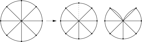
Figure 6. Deletion-contraction on the wheel $W_{8}$.

The classes of the lemon graphs are given by the following result, which we formulate in terms of an algebraic generating function.

Theorem 5.10.

The classes ${\mathbb{U}}(\Lambda_{m})$ are determined by

(5.20) $$\sum_{m\geq 0}{\mathbb{U}}(\Lambda_{m})\,s^{m}=\frac{{\mathbb{T}}+1}{1-{\mathbb{T}}({\mathbb{T}}+1)s-{\mathbb{T}}({\mathbb{T}}+1)^{2}s^{2}}.$$

Proof.

The theorem is proved by setting up a recursion, based on the fact that the $(m+1)$-st lemon graph may be obtained from the $m$-th one by doubling one edge and splitting the newly created edge, as shown in Figure 7.

Figure 7. Lemon building from edge doubling.

Doubling the edge requires handling the graphs obtained by deleting and contracting that edge as shown in Figure 8. These are inductively known:

$${\mathbb{U}}(\Lambda_{m}\smallsetminus e)=({\mathbb{T}}+1){\mathbb{U}}(\Lambda_{m-1})\ \ \ \text{ and }\ \ \ {\mathbb{U}}(\Lambda_{m}/e)={\mathbb{U}}(\Lambda_{m})/({\mathbb{T}}+1),$$

since adding a tail and splitting edges both have the effect of multiplying the motivic class by $({\mathbb{T}}+1)$, as shown in [3], §2.2.

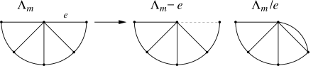
Figure 8. Edge doubling in terms of deletion and contraction.

Applying Lemma 5.2, with $\Lambda_{m}^{\prime}$ denoting the second graph of Figure 7, we obtain

$${\mathbb{U}}(\Lambda_{m+1}) =({\mathbb{T}}+1){\mathbb{U}}(\Lambda^{\prime}_{m})$$

$$=({\mathbb{T}}+1)\left(({\mathbb{T}}-1){\mathbb{U}}(\Lambda_{m})+{\mathbb{T}}{\mathbb{U}}(\Lambda_{m}\smallsetminus e)+({\mathbb{T}}+1){\mathbb{U}}(\Lambda_{m}/e)\right)$$

$$=({\mathbb{T}}+1)\left(({\mathbb{T}}-1){\mathbb{U}}(\Lambda_{m})+{\mathbb{T}}({\mathbb{T}}+1){\mathbb{U}}(\Lambda_{m-1})+{\mathbb{U}}(\Lambda_{m})\right)$$

$$={\mathbb{T}}({\mathbb{T}}+1){\mathbb{U}}(\Lambda_{m})+{\mathbb{T}}({\mathbb{T}}+1)^{2}{\mathbb{U}}(\Lambda_{m-1}).$$

This recursive relation holds as soon as the edge $e$ is not a bridge, that is, for $m\geq 1$. The seeds are $\Lambda_{0}$ (a single edge) and $\Lambda_{1}$ (a triangle), for which we have

$${\mathbb{U}}(\Lambda_{0})={\mathbb{T}}+1\ \ \ \text{ and }\ \ \ {\mathbb{U}}(\Lambda_{1})={\mathbb{T}}({\mathbb{T}}+1)^{2}.$$

Let

$$L_{m}({\mathbb{T}})={\mathbb{U}}(\Lambda_{m}),$$

viewed as a polynomial in ${\mathbb{T}}$, and

$$L(s)=\sum_{m\geq 0}L_{m}s^{m}.$$

The recursion translates into the relation

$$L(s)-{\mathbb{T}}({\mathbb{T}}+1)^{2}s-({\mathbb{T}}+1)$$

$$={\mathbb{T}}({\mathbb{T}}+1)s(L(s)-({\mathbb{T}}+1)+{\mathbb{T}}({\mathbb{T}}+1)^{2}L(s).$$

Solving for $L(s)$ yields the formula (5.20) in the statement. ∎

Equivalently, one can write the reciprocal of the generating function of (5.20) of Theorem 5.10, which has the simpler form

$$\frac{{\mathbb{T}}+1}{\sum_{m\geq 0}{\mathbb{U}}(\Lambda_{m})s^{m}}=1-{\mathbb{T}}({\mathbb{T}}+1)s-{\mathbb{T}}({\mathbb{T}}+1)^{2}s^{2}.$$

We then obtain from Theorem 5.10 an explicit formula for the classes ${\mathbb{U}}(\Lambda_{m})$ in the following way.

Proposition 5.11.

The classes ${\mathbb{U}}(\Lambda_{m})$ are of the form

(5.21) $${\mathbb{U}}(\Lambda_{m})=({\mathbb{T}}+1)^{m+1}K({\mathbb{T}}),$$

where $K({\mathbb{T}})$ is of the form

$$\binom{m}{0}{\mathbb{T}}^{m}+\binom{m-1}{1}{\mathbb{T}}^{m-1}+\binom{m-2}{2}{\mathbb{T}}^{m-2}+\binom{m-3}{3}{\mathbb{T}}^{m-3}+\cdots$$

where $\binom{j}{i}$ is taken to be equal to $0$ if $i>j$.

Proof.

Consider the recurrence relation

$$a_{m}=a_{m-1}+x\,a_{m-2}\quad,\quad m\geq 2$$

with $a_{0}=a_{1}=1$. This is a simple generalization of the Fibonacci sequence, which one recovers for $x=1$. Letting $A(t):=\sum_{m\geq 0}a_{m}t^{m}$, the recurrence gives

$$A(t)-1-t=t(A(t)-1)+x\,t^{2}A(t),$$

hence

$$A(t)=\frac{1}{1-t-x\,t^{2}}.$$

This yields an explicit expression for $a_{m}$: since

$$A(t)=\sum_{k\geq 0}(1+xt)^{k}t^{k}=\sum_{k\geq 0}\sum_{i=0}^{k}\binom{k}{i}t^{i+k}=\sum_{m\geq 0}\,\,\sum_{i\geq 0,i\leq m-i}\binom{m-i}{i}x^{i}t^{m},$$

we get the expression

$$a_{m}=\sum_{i=0}^{m}\binom{m-i}{i}x^{i},$$

adopting the convention that $\binom{j}{i}=0$ if $i>j$. For the classes ${\mathbb{U}}(\Lambda_{m})$ of the lemon graphs we have from Theorem 5.10 the generating function

$$\frac{{\mathbb{T}}+1}{1-{\mathbb{T}}({\mathbb{T}}+1)s-{\mathbb{T}}({\mathbb{T}}+1)^{2}s^{2}}=({\mathbb{T}}+1)\frac{1}{1-({\mathbb{T}}({\mathbb{T}}+1)s)-\frac{1}{{\mathbb{T}}}({\mathbb{T}}({\mathbb{T}}+1)s)^{2}}.$$

Thus, upon setting $t={\mathbb{T}}({\mathbb{T}}+1)s$ and $x=1/{\mathbb{T}}$, the previous considerations give

$${\mathbb{U}}(\Lambda_{m})=({\mathbb{T}}+1)\left(\sum_{i\geq 0}\binom{m-i}{i}\frac{1}{{\mathbb{T}}^{i}}\right){\mathbb{T}}^{m}({\mathbb{T}}+1)^{m}$$

$$=({\mathbb{T}}+1)^{m+1}\sum_{i=0}^{m}\binom{m-i}{i}{\mathbb{T}}^{m-i},$$

which gives (5.21). ∎

As we have seen in the proof of Proposition 5.11 above, the classes ${\mathbb{U}}(\Lambda_{m})$ are closely related to a Fibonacci-like recursion. In fact, they satsify the following property, which is the analog of the well known property of Fibonacci numbers.

Corollary 5.12.

The sequence $a_{m}={\mathbb{U}}(\Lambda_{m-1})$ is a divisibility sequence.

Proof.

A sequence $a_{m}$ is a divisibility sequence if $a_{m}|a_{n}$ whenever $m|n$. We show that the expression for ${\mathbb{U}}(\Lambda_{m-1})$ divides the expression for ${\mathbb{U}}(\Lambda_{n-1})$ if $m$ divides $n$. Using the recursion relation, this follows by showing that if

$$\frac{t}{1-t-xt^{2}}=\sum_{n\geq 0}b_{n}(x)t^{n}$$

then, if $m$ divides $n$, then the polynomial $b_{m}(x)$ divides the polynomial $b_{n}(x)$. The $t$ in the numerator produces the shift of one in the indices.

The polynomials

$$b_{n}(x)=a_{n-1}(x)=\sum_{i=0}^{n-1}\binom{n-1-i}{i}x^{i}$$

can also be written in the form

(5.22) $$b_{m}(x)=\frac{\lambda_{1}^{m}-\lambda_{2}^{m}}{\lambda_{1}-\lambda_{2}}$$

where

$$\lambda_{1}=\frac{1+\sqrt{1+4x}}{2}\ \ \ \text{ and }\ \ \ \lambda_{2}=\frac{1-\sqrt{1+4x}}{2}.$$

Then

$$\frac{b_{km}(x)}{b_{m}(x)}=\frac{\lambda_{1}^{km}-\lambda_{2}^{km}}{\lambda_{1}^{m}-\lambda_{2}^{m}}=\lambda_{1}^{(k-1)m}+\cdots+\lambda_{2}^{(k-1)m}$$

is clearly a polynomial. One can explicitly provide a recurrence relation satisfied by the function of $k$ given by $b^{(m)}_{k}=b_{km}(x)/b_{m}(x)$. First note that $\lambda_{1}^{m}$, $\lambda_{2}^{m}$ are roots of a quadratic polynomial

$$(y-\lambda_{1}^{m})(y-\lambda_{2}^{m})=y^{2}-TY+N=0,$$

where $T=\lambda_{1}^{m}+\lambda_{2}^{m}$ and $N=(\lambda_{1}\lambda_{2})^{m}=(-x)^{m}$. Notice then that

$$\sum_{m\geq 0}(\lambda_{1}^{m}+\lambda_{2}^{m})t^{m}=\frac{1}{1-\lambda_{1}t}+\frac{1}{1-\lambda_{2}t}$$

$$=\frac{2-t}{1-t+t^{2}}=\sum_{m\geq 0}(2b_{m+1}(x)-b_{m}(x))t^{m}.$$

This shows that $T=2b_{m+1}(x)-b_{m}(x)$. Therefore

$$(y-\lambda_{1}^{m})(y-\lambda_{2}^{m})=y^{2}-(2b_{m+1}(x)-b_{m}(x))y+(-x)^{m}\quad.$$

It follows that $b^{(m)}_{k}(x):=\frac{b_{km}(x)}{b_{m}(x)}=\frac{\lambda_{1}^{km}-\lambda_{2}^{km}}{\lambda_{1}^{m}-\lambda_{2}^{m}}$ are solutions of the recurrence relation

$$b^{(m)}_{k+1}=(2b_{m+1}(x)-b_{m}(x))b^{(m)}_{k}-(-x)^{m}b^{(m)}_{k-1}\quad,$$

with seeds $b^{(m)}_{0}=0$, $b^{(m)}_{1}=1$. ∎

In terms of understanding explicitly the motivic nature of the graph hypersurfaces for certain infinite families of graphs, the result of Theorem 5.10, together with Lemma 5.9, has the following direct consequence.

Corollary 5.13.

All graphs $\Gamma$ that are polygon chains have graph hypersurfaces $X_{\Gamma}$ whose classes $[X_{\Gamma}]$ in the Grothendieck ring are contained in the Tate subring ${\mathbb{Z}}[{\mathbb{L}}]\subset K_{0}({\mathcal{V}})$.

5.5. Graph lemonade

As a variation on the same theme explored here, one can compute the class of the graph obtained from any graph $\Gamma$ by ‘building a lemon’ on a given edge $e$, as in Figure 9.

Figure 9. Adding a lemon to a graph.

The question makes no sense if $e$ is a looping edge, and is covered by multiplicativity if $e$ is a bridge, so we can assume that $e$ is not either. One obtains then a formula expressing the class of the “lemonade” of the graph $\Gamma$ at the edge $e$ in terms of ${\mathbb{U}}(\Gamma)$, ${\mathbb{U}}(\Gamma\smallsetminus e)$, ${\mathbb{U}}(\Gamma/e)$.

Proposition 5.14.

Let $e$ be an edge of a graph $\Gamma$, and assume that $e$ is neither a bridge nor a looping edge. Let $\Gamma^{\Lambda}_{m}$ be the “lemonade graph” obtained by building an $m$-lemon fanning out from $e$. Then

$$\sum_{m\geq 0}{\mathbb{U}}(\Gamma^{\Lambda}_{m})s^{m}=\frac{1}{1-{\mathbb{T}}({\mathbb{T}}+1)s-{\mathbb{T}}({\mathbb{T}}+1)^{2}s^{2}}\\ \cdot\left((1-({\mathbb{T}}+1)s)\,{\mathbb{U}}(\Gamma)+({\mathbb{T}}+1){\mathbb{T}}s\,{\mathbb{U}}(\Gamma\smallsetminus e)+({\mathbb{T}}+1)^{2}s\,{\mathbb{U}}(\Gamma/e)\right).$$

Proof.

Let $f_{m}$, $g_{m}$, $h_{m}$ be functions of ${\mathbb{T}}$ such that

$${\mathbb{U}}(\Gamma^{\Lambda}_{m})=f_{m}({\mathbb{T}}){\mathbb{U}}(\Gamma)+g_{m}({\mathbb{T}}){\mathbb{U}}(\Gamma\smallsetminus e)+h_{m}({\mathbb{T}}){\mathbb{U}}(\Gamma/e).$$

The basic recursion is precisely the one worked out in the proof of Theorem 5.10. Namely,

$${\mathbb{U}}(\Lambda_{m+1})={\mathbb{T}}({\mathbb{T}}+1){\mathbb{U}}(\Lambda_{m})+{\mathbb{T}}({\mathbb{T}}+1)^{2}{\mathbb{U}}(\Lambda_{m-1}).$$

This makes sense for $m\geq 1$. The individual functions $f_{m}$, $g_{m}$, $h_{m}$ satisfy this same recursion, but with different seeds:

$$\begin{cases}f_{0}({\mathbb{T}})=1\quad,&f_{1}({\mathbb{T}})={\mathbb{T}}^{2}-1\\ g_{0}({\mathbb{T}})=0\quad,&g_{1}({\mathbb{T}})={\mathbb{T}}({\mathbb{T}}+1)\\ h_{0}({\mathbb{T}})=0\quad,&h_{1}({\mathbb{T}})=({\mathbb{T}}+1)^{2}.\end{cases}$$

The values in the second column implement the doubling formula of Lemma 5.2, and then split the new edge by introducing a factor of ${\mathbb{T}}+1$. Letting $F(s)$, $G(s)$, $H(s)$ be the three corresponding generating functions $F(s)=\sum_{m\geq 0}f_{m}s^{m}$, etc., the recursions imply

$$F(s)-({\mathbb{T}}^{2}-1)s-1 ={\mathbb{T}}({\mathbb{T}}+1)s(F(s)-1)+{\mathbb{T}}({\mathbb{T}}+1)^{2}s^{2}F(s)$$

$$G(s)-{\mathbb{T}}({\mathbb{T}}+1)s ={\mathbb{T}}({\mathbb{T}}+1)sG(s)+{\mathbb{T}}({\mathbb{T}}+1)^{2}s^{2}G(s)$$

$$H(s)-({\mathbb{T}}+1)^{2}s ={\mathbb{T}}({\mathbb{T}}+1)sH(s)+{\mathbb{T}}({\mathbb{T}}+1)^{2}s^{2}H(s)$$

from which

$$F(s) =\frac{1-({\mathbb{T}}+1)s}{1-{\mathbb{T}}({\mathbb{T}}+1)s-{\mathbb{T}}({\mathbb{T}}+1)^{2}s^{2}},$$

$$G(s) =\frac{({\mathbb{T}}+1){\mathbb{T}}s}{1-{\mathbb{T}}({\mathbb{T}}+1)s-{\mathbb{T}}({\mathbb{T}}+1)^{2}s^{2}},$$

$$H(s) =\frac{({\mathbb{T}}+1)^{2}s}{1-{\mathbb{T}}({\mathbb{T}}+1)s-{\mathbb{T}}({\mathbb{T}}+1)^{2}s^{2}},$$

as stated. ∎

The three functions $F(s)$, $G(s)$, $H(s)$ are all easily recoverable from the lemon formula of Theorem 5.10.

Notice, moreover, that the result of Proposition 5.14 yields immediately the following generating series for the Euler characteristic of the complement of $X_{\Gamma^{\Lambda}_{m}}$, valid under the same hypotheses of the proposition. If $\Gamma\smallsetminus e$ is not a forest, then

$$\sum_{m\geq 0}\chi_{\Gamma^{\Lambda}_{m}}s^{m}=(1-s)\,\chi_{\Gamma}+\chi_{\Gamma/e}.$$

That is, $\chi_{\Gamma^{\Lambda}_{1}}=\chi_{\Gamma/e}-\chi_{\Gamma}$ and $\chi_{\Gamma^{\Lambda}_{m}}=0$ for $m>1$.

6. Universal recursion relation

The very structure of the problems analyzed in the previous section is recursive, and this fact alone is responsible for some of the features of the solutions found in §5. We emphasize these general features in this section, and apply them to formulate a precise conjecture for the effect of the operation of multiplying edges on the polynomial invariant $C_{\Gamma}(T)$ of graphs obtained in [3] in terms of CSM classes; recall that we have shown in §3.3 that this is not a specialization of the Tutte polynomial.

6.1. Recursions from multiplying edges

Let $\Gamma$ be a graph with two (possibly coincident) marked vertices $v$, $w$ in the same connected component. Typically, the vertices will be the boundary of an edge $e$ of $\Gamma$. We consider the operation $\Gamma\leadsto\Gamma^{(m)}$ which has the effect of inserting $m$ parallel edges joining $v$ and $w$. Note that obviously $\Gamma^{(m+n)}=(\Gamma^{(m)})^{(n)}$. A feature of invariants $U$ such as the Tutte polynomial and the motivic Feynman rule ${\mathbb{U}}$ is that if $e$ is an edge joining $v$ and $w$ in $\Gamma$, so that $\Gamma^{(m)}=\Gamma_{(m+1)e}$ with the notation of §5.1 and §5.2, then the effect of this operation on $U$ can be expressed consistently as

$$U(\Gamma^{(m)})=f_{m+1}U(\Gamma)+g_{m+1}U(\Gamma\smallsetminus e)+h_{m+1}U(\Gamma/e)\quad.$$

The consistency requirement may be formulated as follows. Let ${\mathcal{R}}$ be the target of the invariant $U$, and consider the evaluation map ${\mathcal{R}}^{\oplus 3}\to{\mathcal{R}}$ given by

$$\begin{pmatrix}g\\ f\\ h\end{pmatrix}\mapsto g\,U(\Gamma\smallsetminus e)+f\,U(\Gamma)+h\,U(\Gamma/e)\quad;$$

then the main requirement is that the effect of $\Gamma\leadsto\Gamma^{(m)}$ can be lifted to a representation of the additive monoid ${\mathbb{Z}}^{\geq 0}$ on ${\mathcal{R}}^{\oplus 3}$. In other words, these operations may be represented by $3\times 3$ matrices $A_{m}$, such that

$$A_{m}\cdot\begin{pmatrix}0\\ 1\\ 0\end{pmatrix}=\begin{pmatrix}g_{m+1}\\ f_{m+1}\\ h_{m+1}\end{pmatrix}\mapsto f_{m+1}U(\Gamma)+g_{m+1}U(\Gamma\smallsetminus e)+h_{m+1}U(\Gamma/e)=U(\Gamma^{(m)})$$

and $A_{0}=1$, $A_{m+n}=A_{m}\cdot A_{n}$. It is also natural to assume that

$$A_{1}\cdot\begin{pmatrix}0\\ 1\\ 0\end{pmatrix}=\begin{pmatrix}1\\ 0\\ 0\end{pmatrix}\quad,$$

reflecting the fact that $\Gamma=(\Gamma\smallsetminus e)^{(1)}$ (assuming $\Gamma\smallsetminus e$ is marked by $\partial e$), and

$$A_{1}\cdot\begin{pmatrix}0\\ 0\\ 1\end{pmatrix}=\begin{pmatrix}0\\ 0\\ Z\end{pmatrix}\quad,$$

where $Z$ is the value of $U$ on the graph consisting of a single looping edge. This last requirement is motivated by the fact that the endpoints $v$, $w$ of $e$ coincide in the contraction $\Gamma/e$, therefore $(\Gamma/e)^{(1)}$ consists of $\Gamma/e$ with a looping edge attached to $v=w$; since $U$ is a Feynman rule, the effect must amount to simple multiplication by $Z$.

The datum of the representation is captured by the generating function

$$A(s):=\sum_{m\geq 0}A_{m}\frac{s^{m}}{m!}=e^{A_{1}s}\quad.$$

Our task is to determine this function, or equivalently the generating functions

$$f(s)=\sum_{m\geq 0}f_{m}\frac{s^{m}}{m!}\quad,\quad g(s)=\sum_{m\geq 0}g_{m}\frac{s^{m}}{m!}\quad,\quad h(s)=\sum_{m\geq 0}h_{m}\frac{s^{m}}{m!}\quad.$$

Here, it is natural to set

(6.1) $$\begin{cases}f_{0}=0\\ f_{1}=1\end{cases}\quad,\quad\begin{cases}g_{0}=1\\ g_{1}=0\end{cases}\quad,\quad\begin{cases}h_{0}=0\\ h_{1}=0\end{cases}\quad.$$

Lemma 6.1.

Let $U$ be a Feynman rule, and assume that $Z$ is the value of $U$ on the graph consisting of a single looping edge. Then for $m\geq 0$

$$A_{m}=\begin{pmatrix}g_{m}&g_{m+1}&0\\ f_{m}&f_{m+1}&0\\ h_{m}&h_{m+1}&Z^{m}\end{pmatrix}$$

and the coefficients $f_{m}$, $g_{m}$, $h_{m}$ satisfy the following recursion

(6.2) $$\begin{cases}f_{m+2}=f_{2}f_{m+1}+g_{2}f_{m}\\ g_{m+1}=g_{2}f_{m}\\ h_{m+1}=h_{2}f_{m}+Zh_{m}\end{cases}$$

for $m\geq 0$.

Proof.

By assumption,

$$A_{m}\cdot\begin{pmatrix}0\\ 1\\ 0\end{pmatrix}=\begin{pmatrix}g_{m+1}\\ f_{m+1}\\ h_{m+1}\end{pmatrix}\quad\text{and}\quad A_{1}=\begin{pmatrix}0&g_{2}&0\\ 1&f_{2}&0\\ 0&h_{2}&Z\end{pmatrix}\quad.$$

Assuming inductively that $A_{m-1}=\begin{pmatrix}g_{m-1}&g_{m}&0\\ f_{m-1}&f_{m}&0\\ h_{m-1}&h_{m}&Z^{m}\end{pmatrix}$, the fact that $A_{m}=A_{m-1}A_{1}$ shows that $A_{m}$ has the stated shape. The recursion is forced by the fact that $A_{m+1}=A_{1}A_{m}$, which gives

$$\begin{pmatrix}g_{m+1}&g_{m+2}&0\\ f_{m+1}&f_{m+2}&0\\ h_{m+1}&h_{m+2}&Z^{m+1}\end{pmatrix} =\begin{pmatrix}0&g_{2}&0\\ 1&f_{2}&0\\ 0&h_{2}&Z\end{pmatrix}\begin{pmatrix}g_{m}&g_{m+1}&0\\ f_{m}&f_{m+1}&0\\ h_{m}&h_{m+1}&Z^{m}\end{pmatrix}$$

$$=\begin{pmatrix}g_{2}f_{m}&g_{2}f_{m+1}&0\\ g_{m}+f_{2}f_{m}&g_{m+1}+f_{2}f_{m+1}&0\\ h_{2}f_{m}+Zh_{m}&h_{2}f_{m+1}+Zh_{m+1}&Z^{m+1}\end{pmatrix}$$

and shows that

$$\begin{cases}f_{m+2}=f_{2}f_{m+1}+g_{m+1}\\ g_{m+1}=g_{2}f_{m}\\ h_{m+1}=h_{2}f_{m}+Zh_{m}\end{cases}.$$

Then (6.2) follows immediately. ∎

In specific cases, the recursion can often be solved by computing explicitly $e^{A_{1}s}$, which is straightforward if $A_{1}$ is diagonalizable. This can be carried out easily for the the motivic Feynman rule, for which

$$A_{1}=\begin{pmatrix}0&{\mathbb{T}}-1&0\\ 1&{\mathbb{T}}&0\\ 0&{\mathbb{T}}+1&{\mathbb{T}}\end{pmatrix}\quad,$$

recovering formula (5.13) in Theorem 5.3. It can also be worked out for the Tutte polynomial, for which we can choose

(6.3) $$A_{1}=\begin{pmatrix}0&1&0\\ 1&0&0\\ 0&1+y&y\end{pmatrix}.$$

Since the Tutte polynomial satisfies the relation $T_{\Gamma}=T_{\Gamma\smallsetminus e}+T_{\Gamma/e}$, there are in fact many possible choices for the corresponding representation. The one chosen in (6.3) gives

$$A(s)=\sum_{m\geq 0}A_{m}\frac{s^{m}}{m!}=\begin{pmatrix}0&\frac{1-y}{1+y}&1\\ 0&\frac{1-y}{1+y}&-1\\ 1&1&1\end{pmatrix}\begin{pmatrix}e^{ys}&0&0\\ 0&e^{s}&0\\ 0&0&e^{-s}\end{pmatrix}\begin{pmatrix}\frac{1}{y-1}&\frac{y}{y-1}&1\\ \frac{1}{2}\frac{1+y}{1-y}&\frac{1}{2}\frac{1+y}{1-y}&0\\ \frac{1}{2}&-\frac{1}{2}&0\end{pmatrix}$$

and correspondingly

$$\begin{array}[]{rl}f(s)=&\displaystyle{\frac{e^{s}-e^{-s}}{2}}=\sinh s\\[8.53581pt] g(s)=&\displaystyle{\frac{e^{s}+e^{-s}}{2}}=\cosh s\\[8.53581pt] h(s)=&\displaystyle{\frac{e^{ys}-e^{s}}{y-1}-\sinh s}.\end{array}$$

Since the deletion–contraction relation (2.15) holds, this is equivalent to the result of Proposition 5.1.

The recursion (6.2) can be solved directly in general by the same method for the specific cases analyzed in §5. The conditions translate into differential equations satisfied by the functions $f$, $g$, $h$, and specifically

(6.4) $$\left\{\begin{aligned} f^{\prime\prime}(s)&=f_{2}\,f^{\prime}(s)+g_{2}f(s)\\ g^{\prime}(s)&=g_{s}\,f(s)\\ h^{\prime}(s)&=Z\,h(s)+h_{2}\,f(s)\end{aligned}\right.\quad.$$

With the initial conditions specified in (6.1), and assuming $f_{2}^{2}+4g_{2}\neq 0$, the first equation has the solution

$$f(s)=\frac{e^{\lambda_{+}s}-e^{\lambda_{-}s}}{\lambda_{+}-\lambda_{-}}\quad,\quad\text{where $\lambda_{\pm}=\frac{f_{2}\pm\sqrt{f_{2}^{2}+4g_{2}}}{2}$}\quad;$$

equivalently,

$$f_{m}=\frac{\lambda_{+}^{m}-\lambda_{-}^{m}}{\lambda_{+}-\lambda_{-}}=\lambda_{+}^{m-1}+\lambda_{+}^{m-2}\lambda_{-}+\cdots+\lambda_{-}^{m-1}\quad.$$

The second and third equations then determine $g$ and $h$:

$$g(s)=\frac{\lambda_{+}e^{\lambda_{-}s}-\lambda_{-}e^{\lambda_{+}s}}{\lambda_{+}-\lambda_{-}}$$

and

$$h(s)=\frac{h_{2}}{\lambda_{+}-\lambda_{-}}\left(\frac{e^{\lambda_{+}s}-e^{Zs}}{\lambda_{+}-Z}-\frac{e^{\lambda_{-}s}-e^{Zs}}{\lambda_{-}-Z}\right)$$

if $\lambda_{+}\neq Z$ and $\lambda_{-}\neq Z$, while

$$h(s)=\frac{h_{2}}{Z-\lambda}\left(s\,e^{Zs}-\frac{e^{Zs}-e^{\lambda s}}{Z-\lambda}\right)$$

if $\{\lambda_{+},\lambda_{-}\}=\{Z,\lambda\}$. This last eventuality occurs for the motivic Feynman rule.

The equations (6.4) highlight interesting features of the coefficients of any solution to the multiplying edge problem, independent of the specific context. From the general solution, we also see that

$$\frac{f(s)}{g(s)}=\frac{e^{\lambda_{+}s}-e^{\lambda_{-}s}}{\lambda_{+}e^{\lambda_{-}s}-\lambda_{-}e^{\lambda_{+}s}}\quad,$$

generalizing Remark 5.4. For the Tutte polynomial (with the choice of (6.3)) this function is the hyperbolic tangent.

As a last general remark, we note that the coefficients $f_{m}$ form a divisibility sequence. This is clear from the expression for $f_{m}$ given above: $f^{(m)}_{r}:=\frac{f_{rm}(s)}{f_{m}(s)}=\frac{\lambda_{+}^{rm}-\lambda_{-}^{rm}}{\lambda_{+}^{m}-\lambda_{-}^{m}}$. Alternatively, it can be proved as in Corollary 5.12: one finds that the quotients $f^{(m)}_{r}$ satisfy the recursion

$$f^{(m)}_{r+2}=(f_{2}f_{m}+2g_{2}f_{m-1})f^{(m)}_{r+1}-(-g_{2})^{m}f^{(m)}_{r}\quad,$$

for all $r\geq 0$, and in particular it follows that $f_{m}(s)$ divides $f_{rm}(s)$ for all $r\geq 0$.

6.2. Conjectural behavior of $C_{\Gamma}$ under multiplication of edges

A deletion/contraction rule for the invariant $C_{\Gamma}$ is not yet available; however, if such a rule exists then a doubling-edge formula for this invariant should exist, of the type considered above: if $e$ is an edge of $\Gamma$ joining the marked vertices, then one would expect

$$C_{\Gamma^{(m)}}\overset{?}{=}f_{m+1}\cdot C_{\Gamma}+g_{m+1}\cdot C_{\Gamma\smallsetminus e}+h_{m+1}\cdot C_{\Gamma/e}$$

for suitable coefficients satisfying the stringent requirements examined in §6.1. The fact that $C_{\Gamma}$ is known for banana graphs (Example 3.8 in [3]) provides then a testing ground for this phenomenon, as well as a precise indication for what the needed representation should be in this case.

Conjecture 6.1.

The polynomial Feynman rule $C_{\Gamma}$ obeys the general recursion formulas obtained in §6.1 with respect to the operation of multiplying edges. The corresponding representation is determined by

$$f_{2}=2T-1,\ \ \ \ g_{2}=-T(T-1),\ \ \ \ h_{2}=1\quad.$$

The generating functions for the operation are

$$\begin{array}[]{rl}f(s)=&e^{Ts}-e^{(T-1)s}\\[8.53581pt] g(s)=&Te^{(T-1)s}-(T-1)e^{Ts}\\[8.53581pt] h(s)=&e^{(T-1)s}+(s-1)e^{Ts}.\end{array}$$

Since the Euler characteristic $\chi_{\Gamma}$ of the complement of $X_{\Gamma}$ in its ambient projective space can be recovered from $C_{\Gamma}$ (cf. Proposition 3.1 in [3]), these formulae imply generating functions for $\chi_{\Gamma^{(m)}}$. These coincide with the formulae obtained in Corollary 5.5, providing some evidence for Conjecture 6.1.

Conjecture 6.1 is verified for all cases known to us: the family of banana graphs, as well as several examples for small graphs computed by J. Stryker ([33]). In fact, the smallest graph for which the invariant $C_{\Gamma}(T)$ is not known is the triangle with doubled edges; according to Conjecture 6.1, the polynomial invariant for this graph is

$$T^{6}+2T^{5}+8T^{4}+2T^{3}+T^{2}-T\quad,$$

and it follows that the CSM class of the corresponding graph hypersurface should be

$$4[{\mathbb{P}}^{4}]+7[{\mathbb{P}}^{3}]+18[{\mathbb{P}}^{2}]+14[{\mathbb{P}}]+7[{\mathbb{P}}^{0}]\quad.$$

7. Categorification

Various examples of categorifications of graph and link invariants have been recently developed. These are categorical constructions with associated (co)homology theories, from which the (polynomial) invariant is recontructed as Euler characteristic. The most famous examples of categorification are Khovanov homology [26], which is a categorification of the Jones polynomial, and graph homology, which gives a categorification of the chromatic polynomial [21]. More recently, a categorification of the Tutte polynomial was also introduced in [25]. In the known categorifications of invariants obtained from specializations of the Tutte polynomial, the deletion–contraction relations manifest themselves in the form of long exact (co)homology sequences. Another way in which the notion of categorification found applications to algebraic structures associated to graphs is in the context of Hall algebras. In this context, one looks for a categorification of a Hopf algebra, that is, an abelian category such that the given Hopf algebra is the assoctaed Hall–Ringel algebra. In the case of the Connes–Kreimer Hopf algebra of Feynman graphs, a suitable categorification, which realizes it (or rather its dual Hopf algebra) as a Ringel–Hall algebra, was recently obtained in [28].

In view of all these results on categorification, it seems natural to try to interpret the deletion–contraction relation described in this paper for the motivic Feynman rules in terms of a suitable categorification. As remarked in §8 of [7], one can think of the motive associated to the graph $\Gamma$ and the maps induced by edge contractions as a motivic version of graph cohomology. We see a similar setting here in terms of the deletion–contraction relations we obtained in §3 and §4.

We denote by ${\mathfrak{m}}(X)$ the motive of a variety $X$, seen as an object in the triangulated category ${\mathcal{D}}{\mathcal{M}}_{\mathbb{Q}}$ of mixed motives of [35]. A closed embedding $Y\subset X$ determines a distinguished triangle in this category

(7.1) $${\mathfrak{m}}(Y)\to{\mathfrak{m}}(X)\to{\mathfrak{m}}(X\smallsetminus Y)\to{\mathfrak{m}}(Y)[1].$$

Since one thinks of motives as a universal cohomology theory for algebraic varieties, and of classes in the Grothendieck ring as a universal Euler characteristic, it is natural to view the motive ${\mathfrak{m}}(X_{\Gamma})\in{\mathcal{D}}{\mathcal{M}}_{\mathbb{Q}}$ as the “categorification” of the “Euler characteristic” $[X_{\Gamma}]\in K_{0}({\mathcal{V}}_{\mathbb{Q}})$.

The analog of the fact that the categorification of deletion–contraction relations takes the form of long exact cohomology sequences is then expressed in this context in the following way.

Proposition 7.1.

For a graph $\Gamma$ with $n$ edges, let ${\mathfrak{m}}_{\Gamma}:={\mathfrak{m}}({\mathbb{P}}^{n-1}\smallsetminus X_{\Gamma})$ as an object in ${\mathcal{D}}{\mathcal{M}}_{\mathbb{Q}}$. The deletion contraction relation of Theorem 3.8 determines a distinguished triangle in ${\mathcal{D}}{\mathcal{M}}_{\mathbb{Q}}$ of the form

(7.2) $${\mathfrak{m}}_{\Gamma\smallsetminus e}\to{\mathfrak{m}}_{\Gamma}\to{\mathfrak{m}}({\mathbb{P}}^{n-1}\smallsetminus(\overline{X_{\Gamma\smallsetminus e}}\cap\overline{X_{\Gamma/e}}))\to{\mathfrak{m}}_{\Gamma\smallsetminus e}[1],$$

where, as above $\overline{X}$ denotes the cone on $X$.

Proof.

This follows from the proof of Theorem 3.8. In fact, for the inclusion $X_{\Gamma}\smallsetminus(X_{\Gamma}\cap\overline{X_{\Gamma\smallsetminus e}})$ in ${\mathbb{P}}^{n-1}\smallsetminus X_{\Gamma}$, we have a distringuished triangle of the form

$${\mathfrak{m}}(X_{\Gamma}\smallsetminus(X_{\Gamma}\cap\overline{X_{\Gamma\smallsetminus e}}))\to{\mathfrak{m}}({\mathbb{P}}^{n-1}\smallsetminus X_{\Gamma})$$

$$\to{\mathfrak{m}}({\mathbb{P}}^{n-1}\smallsetminus(X_{\Gamma}\cap\overline{X_{\Gamma\smallsetminus e}}))\to{\mathfrak{m}}(X_{\Gamma}\smallsetminus(X_{\Gamma}\cap\overline{X_{\Gamma\smallsetminus e}}))[1].$$

We then use the isomorphisms

$$X_{\Gamma}\smallsetminus(X_{\Gamma}\cap\overline{X_{\Gamma\smallsetminus e}})\simeq{\mathbb{P}}^{n-2}\smallsetminus X_{\Gamma\smallsetminus e}$$

and

$$X_{\Gamma}\cap\overline{X_{\Gamma\smallsetminus e}}\simeq\overline{X_{\Gamma/e}}\cap\overline{X_{\Gamma\smallsetminus e}}$$

proved in Theorem 3.8 to get the triangle (7.2). ∎

This means that we can upgrade at the level of the category ${\mathcal{D}}{\mathcal{M}}_{\mathbb{Q}}$ of mixed motives some of the arguments that we formulated in the previous sections at the level of classes in the Grothendieck ring of varieties.

Corollary 7.2.

Let $\Gamma_{me}$ denote the graph obtained from a given graph $\Gamma$ by replacing an edge $e$ by $m$ parallel edges, as in §5.2. If ${\mathfrak{m}}_{\Gamma}$, ${\mathfrak{m}}_{\Gamma\smallsetminus e}$ and ${\mathfrak{m}}_{\Gamma/e}$ belong to the sub-triangulated category ${\mathcal{D}}{\mathcal{M}}{\mathcal{T}}_{\mathbb{Q}}\subset{\mathcal{D}}{\mathcal{M}}_{\mathbb{Q}}$ of mixed Tate motives, then the motive ${\mathfrak{m}}_{\Gamma_{me}}$ also belongs to ${\mathcal{D}}{\mathcal{M}}{\mathcal{T}}_{\mathbb{Q}}$.

Proof.

It suffices to show that the result holds for $\Gamma_{2e}$. We look at the case where $e$ is neither a bridge nor a looping edge. The other cases can be handled similarly. One follows the same argument of Proposition 5.2, written in terms of the distinguished triangle (7.2), which is here of the form

$${\mathfrak{m}}_{\Gamma}\to{\mathfrak{m}}_{\Gamma_{2e}}\to{\mathfrak{m}}({\mathbb{P}}^{n-1}\smallsetminus(\overline{X_{\Gamma}}\cap\overline{X_{\Gamma_{o}}}))\to{\mathfrak{m}}_{\Gamma}[1],$$

where $\Gamma_{o}$ is the graph obtained by attaching a looping edge at the vertex $e$ is contracted to in the graph $\Gamma/e$. Since ${\mathcal{D}}{\mathcal{M}}{\mathcal{T}}_{\mathbb{Q}}$ is a sub-triangulated category of ${\mathcal{D}}{\mathcal{M}}_{\mathbb{Q}}$, to know that ${\mathfrak{m}}_{\Gamma_{2e}}$ is (isomorphic to) an object in ${\mathcal{D}}{\mathcal{M}}{\mathcal{T}}_{\mathbb{Q}}$ it suffices to know that the remaining two terms of the distinguished triangle belong to ${\mathcal{D}}{\mathcal{M}}{\mathcal{T}}_{\mathbb{Q}}$. This requires expressing ${\mathfrak{m}}({\mathbb{P}}^{n-1}\smallsetminus(\overline{X_{\Gamma}}\cap\overline{X_{\Gamma_{o}}}))$ in terms of mixed Tate motives. This can be done again as in Proposition 5.2, using again (5.10) to control the term ${\mathfrak{m}}({\mathbb{P}}^{n-1}\smallsetminus(\overline{X_{\Gamma}}\cap\overline{X_{\Gamma_{o}}}))$ in terms of another distinguished triangle involving ${\mathfrak{m}}_{\Gamma\smallsetminus e}$ and ${\mathfrak{m}}_{\Gamma/e}$. ∎

Similarly, we can lift at this motivic level the statement of Corollary 5.13 and the construction of the “lemonade graphs” of §5.5.

Corollary 7.3.

The motives ${\mathfrak{m}}_{\Gamma}$ of graphs $\Gamma$ that are polygon chains belong to the subcategory ${\mathcal{D}}{\mathcal{M}}{\mathcal{T}}_{\mathbb{Q}}$ of mixed Tate motives. Moreover, if $\Gamma$ is a graph such that ${\mathfrak{m}}_{\Gamma}$, ${\mathfrak{m}}_{\Gamma\smallsetminus e}$, and ${\mathfrak{m}}_{\Gamma/e}$ are onjects in the subcategory ${\mathcal{D}}{\mathcal{M}}{\mathcal{T}}_{\mathbb{Q}}$ of mixed Tate motives, all the graphs of the form $\Gamma^{\Lambda}_{m}$, obtained as in Proposition 5.14 by attaching a lemon graph to the edge $e$ also have ${\mathfrak{m}}_{\Gamma^{\Lambda}_{m}}$ in ${\mathcal{D}}{\mathcal{M}}{\mathcal{T}}_{\mathbb{Q}}$.

Another possible way of formulation the deletion–contraction relations of Theorem 3.8 at the level of the triangulated category of mixed motives, in the form of distinguished triangles, would be to use the geometric description of the deletion–contraction relations given in §4 in terms of the blowup diagram (4.1) and used distinguished triangles in ${\mathcal{D}}{\mathcal{M}}_{\mathbb{Q}}$ associated to blowups.

A related question is then to provide a categorification for the polynomial invariant $C_{\Gamma}(T)$. This ties up with the question of what type of deletion–contraction relation this invariant satisfies by reformulating the question in terms of a possible long exact cohomology sequence.

Acknowledgments. The results in this article were catalyzed by a question posed to the first author by Michael Falk during the Jaca ‘Lib60ber’ conference, in June 2009. We thank him and the organizers of the conference, and renew our best wishes to Anatoly Libgober. We thank Friedrich Hirzebruch for pointing out Remark 5.4 to us, thereby triggering the thoughts leading to much of the material in §6. We also thank Don Zagier for a useful conversation on divisibility sequences and generating functions. The second author is partially supported by NSF grants DMS-0651925 and DMS-0901221. This work was carried out during a stay of the authors at the Max Planck Institute in July 2009.

References

- [1] P. Aluffi, Chern classes of blow-ups, arXiv:0809.2425, to appear in Math. Proc. Camb. Phil. Soc.
- [2] P. Aluffi, M. Marcolli, Feynman motives of banana graphs, Commun. Number Theory and Phys., Vol.3 (2009) N.1, 1-57.
- [3] P. Aluffi, M. Marcolli, Algebro-geometric Feynman rules, arXiv:0811.2514.
- [4] P. Aluffi, M. Marcolli, Parametric Feynman integrals and determinant hypersurfaces, arXiv:0901.2107.
- [5] P. Belkale, P. Brosnan, Matroids, motives, and a conjecture of Kontsevich, Duke Math. Journal, Vol.116 (2003) 147–188.
- [6] J. Bjorken, S. Drell, Relativistic Quantum Fields, McGraw-Hill, 1965.
- [7] S. Bloch, Motives associated to graphs. Jpn. J. Math. 2 (2007), no. 1, 165–196.
- [8] S. Bloch, H. Esnault, D. Kreimer, On motives associated to graph polynomials. Comm. Math. Phys. 267 (2006), no. 1, 181–225.
- [9] S. Bloch, D. Kreimer, Mixed Hodge structures and renormalization in physics. Commun. Number Theory Phys., Vol.2 (2008), no. 4, 637–718.
- [10] B. Bollobás, Modern graph theory, Springer, 1998.
- [11] D. Broadhurst, D. Kreimer, Association of multiple zeta values with positive knots via Feynman diagrams up to 9 loops, Phys. Lett. B, Vol.393 (1997) 403–412.
- [12] F. Brown, The massless higher-loop two-point function, Commun. Math. Phys., Vol.287 (2009) 925–958.
- [13] T.H. Brylawski, The Tutte–Grothendieck ring, Algebra Universalis, Vol.2 (1972) N.1, 375–388.
- [14] A. Connes, D. Kreimer, Renormalization in quantum field theory and the Riemann–Hilbert problem I. The Hopf algebra structure of graphs and the main theorem, Comm. Math. Phys., Vol.210 (2000) 249–273.
- [15] A. Connes, D. Kreimer, Renormalization in quantum field theory and the Riemann-Hilbert problem. II. The -function, diffeomorphisms and the renormalization group. Comm. Math. Phys. 216 (2001), no. 1, 215–241.
- [16] A. Connes, M. Marcolli, Renormalization and motivic Galois theory. Int. Math. Res. Not. 2004, no. 76, 4073–4091.
- [17] A. Connes, M. Marcolli, Noncommutative geometry, quantum fields and motives, Colloquium Publications, Vol.55. American Mathematical Society and Hindustan Book Agency, 2008. xxii+785 pp.
- [18] H.H. Crapo, The Tutte polynomial, Aequationes Mathematicae, Vol. 3 (1969) N.3, 211–229.
- [19] D. Doryn, Cohomology of graph hypersurfaces associated to certain Feynman graphs, PhD Thesis, University of Duisburg-Essen, arXiv:0811.0402.
- [20] K. Ebrahimi-Fard, L. Guo, D. Kreimer, Spitzer’s identity and the algebraic Birkhoff decomposition in pQFT. J. Phys. A 37 (2004), no. 45, 11037–11052.
- [21] L. Helme-Guizon, Y. Rong, A categorification for the chromatic polynomial, Alg. Geom. Topology, Vol. 5 (2005) 1365–1388.
- [22] F. Hirzebruch, Topological methods in algebraic geometry, Classics in Mathematics. Springer, 1995. xii+234 pp.
- [23] C. Itzykson, J.B. Zuber, Quantum Field Theory, Dover Publications, 2006.
- [24] F. Jaeger, Tutte polynomials and link polynomials. Proc. Amer. Math. Soc., Vol.103 (1988), no. 2, 647–654.
- [25] E.F. Jasso-Hernandez, Y. Rong, A categorification for the Tutte polynomial, Alg. Geom. Topology, Vol.6 (2006) 2031–2049.
- [26] M. Khovanov, A categorification of the Jones polynomial, Duke Math. J., Vol.101 (2000) 359–426.
- [27] D. Kreimer, The core Hopf algebra, arXiv:0902.1223.
- [28] K. Kremnizer, M. Szczesny, Feynman Graphs, Rooted Trees, and Ringel-Hall Algebras, arXiv:0806.1179.
- [29] M. LeBellac, Quantum and statistical field theory, Oxford Science Publications, 1991.
- [30] M. Marcolli, Motivic renormalization and singularities, arXiv:0804.4824.
- [31] M. Marcolli, Feynman integrals and motives, arXiv:0907.0321, to appear in the Proceedings of the 5th European Congress of Mathematics.
- [32] M. Marcolli, Feynman motives, book to appear, World Scientific, 2009.
- [33] J. Stryker, A list of graph hypersurfaces and their Chern-Schwartz-MacPherson classes, preprint, 2008.
- [34] M.B. Thistlethwaite, A spanning tree expansion of the Jones polynomial, Topology 26 (1987), no. 3, 297–309.
- [35] V. Voevodsky, Triangulated categories of motives over a field. in “Cycles, transfer and motivic homology theories”, pp.188–238, Annals of Mathematics Studies, Vol.143, Princeton University Press, 2000.