Molecular dynamics with quantum heat baths: results for nanoribbons and nanotubes

Abstract

A generalized Langevin equation with quantum baths (QMD) for thermal transport is derived with the help of nonequilibrium Green’s function (NEGF) formulation. The exact relationship of the quasi-classical approximation to NEGF is demonstrated using Feynman diagrams of the nonlinear self energies. To leading order, the retarded self energies agree, but QMD and NEGF differ in lesser/greater self energies. An implementation for general systems using Cholesky decomposition of the correlated noises is discussed. Some means of stabilizing the dynamics are given. Thermal conductance results for graphene strips under strain and temperature dependence of carbon nanotubes are presented. The “quantum correction” method is critically examined.

I Introduction

Molecular dynamicsMDbook (MD) has been used as one of the most important simulation tools to study a variety of problems from structure to dynamics. In particular, MD is routinely used for thermal transport problemslepri03 ; mcgaughey06 . MD is versatile and can handle with ease any form of classical interaction forces. The computer implementation of the algorithms is straightforward in most cases. However, there is one essential drawback in MD – it is purely classical, thus it is unable to predict quantum behavior. Of course, in situations like high temperatures and atoms other than hydrogen, MD gives good approximation. This is not the case for very small systems like nanostructures at low temperatures. For lattice vibrations, the relevant temperature scale is the Debye temperature, which is quite high for carbon-based materials. Thus, even the room temperature of 300 K is already considered a low temperature. One uses MD anyway in cases where quantum effects might be important, for lack of better alternative approaches.

Recently, it was proposed that MD can be augmented with a quantum heat bath to at least partially take into account the quantum effect wangPRL07 . We’ll refer to this new molecular dynamics as QMD. The proposed generalized Langevin dynamics with correlated noise obtained according to Bose distribution has the important features that it gives correct results in two special limits, the low-temperature ballistic limit and high-temperature diffusive limit. It is one of the very few methods that ballistic to diffusive transport can be studied in a single unified framework. The QMD should be most accurate for systems with strong center-lead couplings. The non-Markovian heat baths have an additional advantage in comparison with the usual Langevin or Nosé-Hoover heat baths in that the baths (the leads) and the systems can be connected seamlessly without thermal boundary resistance.

In this paper, we follow up the work of ref. wangPRL07, to give further details and calculations on large systems. We first discuss the implementation of the colored noises with several degrees of freedom. We then discuss the problem of instabilities we encountered in carrying out the simulation. Various ways of overcoming this difficulty are suggested and tested. We analyze the proposed dynamics and compare it with the exact nonequilibrium Green’s function (NEGF) methodwangrev08 in terms of Feynman diagrams and nonlinear self-energies. Here we show that in the ballistic case, the generalized Langevin dynamics and NEGF are completely equivalent. Using this analysis, it is also clear that at high temperatures NEGF and Langevin dynamics should agree for nonlinear systems. We then report some of the simulation results on nanoribbons (with periodic boundary condition in the transverse direction) and nanotubes. We comment on one popular method of “quantum correction” and point out its shortcomings and inconsistencies. We conclude in the last section.

II Generalized Langevin dynamics and implementation details

The derivation of the generalized Langevin equation for junction systems was given in ref. wangPRL07, , see also refs. adelman76, and dharJSP06, . Here we present a much faster derivation using the results of NEGF, following the notations introduced in ref. wangrev08, . The starting point is the set of quantum Heisenberg equations of motion for the leads and center,

$$\ddot{u}^{C} = F^{C}-V^{CL}u^{L}-V^{CR}u^{R},$$ (1)

$$\ddot{u}^{\alpha} = -K^{\alpha}u^{\alpha}-V^{\alpha C}u^{C},\qquad\alpha=L,R.$$ (2)

$u^{\alpha}$ is a vector of displacements in region $\alpha$ away from the equilibrium positions, multiplied by the square root of mass of the atoms. The leads and the coupling between the leads and center are linear; while the force in the center, $F^{C}(u^{C})=-K^{C}u^{C}+F_{n}$, is arbitrary. We eliminate the lead variables by solving the second equation and substituting it back into the first equation. The general solution for the left lead is

$$u^{L}(t)=u_{0}^{L}(t)+\int^{t}\!g^{r}_{L}(t-t^{\prime})\,V^{LC}u^{C}(t^{\prime})\,dt^{\prime},$$ (3)

where $g^{r}_{L}(t)$ is the retarded Green’s function of a free left lead with the spring constant $K^{L}$, satisfying $\ddot{g}^{r}_{L}(t)+K^{L}g^{r}_{L}(t)=-\delta(t)I$, $g^{r}_{L}(t)=0$ for $t\leq 0$. Its Fourier transform is given by $[(\omega+i\eta)^{2}-K^{L}]^{-1}$, where $\eta\to 0^{+}$ is an infinitesimal positive quantity. $u_{0}^{L}(t)$ satisfies the homogeneous equation of the free left lead:

$$\ddot{u}_{0}^{L}+K^{L}u^{L}_{0}=0.$$ (4)

$g^{r}_{L}(t)$ and $u_{0}^{L}(t)$ are associated with the “free” lead in the sense that leads and center are decoupled, as if $V^{CL}=0$. This is consistent with an adiabatic switch-on of the lead-center couplings. The right lead equations are similar. Substituting Eq.(3) into Eq. (1), we obtain

$$\ddot{u}^{C}=F^{C}-\int^{t}\Sigma^{r}(t-t^{\prime})u^{C}(t^{\prime})dt^{\prime}+\xi,$$ (5)

where $\Sigma^{r}=\Sigma_{L}^{r}+\Sigma_{R}^{r}$, $\Sigma_{\alpha}^{r}=V^{C\alpha}g_{\alpha}^{r}(t)V^{\alpha C}$, is the self-energy of the leads, and the noise is defined by $\xi_{\alpha}(t)=-V^{C\alpha}u^{\alpha}_{0}(t)$, $\xi=\xi_{L}+\xi_{R}$.

The most important characterization of the system is the properties of the noises. This is fixed by assuming that the leads are in respective thermal equilibrium at temperature $T_{L}$ and $T_{R}$. It is obvious that for a set of coupled harmonic oscillators, there is no thermal expansion effect, $\langle u_{0}^{\alpha}(t)\rangle=0$, thus $\langle\xi_{\alpha}\rangle=0$. The correlation function of the noise is

$$\langle\xi_{L}(t)\xi_{L}^{T}(t^{\prime})\rangle = V^{CL}\langle u_{0}^{L}(t)u_{0}^{L}(t^{\prime})^{T}\rangle V^{LC}$$ (6)

$$= V^{CL}i\hbar g_{L}^{>}(t-t^{\prime})V^{LC}$$

$$= i\hbar\Sigma_{L}^{>}(t-t^{\prime}),$$

where the superscript $T$ stands for matrix transpose. We have used the definition of greater Green’s function and self-energy of the free left leadwangrev08 . We assume that the noises of the left lead and right lead are independent. Since the noises $\xi_{\alpha}(t)$ are quantum operators, they do not commute in general. In fact, the correlation in the reverse order is given by the lesser self-energy:

$$\langle\xi_{L}(t^{\prime})\xi_{L}^{T}(t)\rangle^{T}=i\hbar\Sigma_{L}^{<}(t-t^{\prime}).$$ (7)

Equation (5) together with the noise correlations Eq. (6) and (7) is equivalent to NEGF approach. For the quantum Langevin equation, it is not sufficient to completely characterize the solution by just the first and second moments of the noises. We need the complete set of $n$-point correlators $\langle\xi(t_{1})\xi(t_{2})\cdots\xi(t_{n})\rangle$, which is in principle calculable from the equilibrium properties of the lead subsystem ford-kac-mazur65 . It is very difficult to solve the dynamics unless the nonlinear force $F_{n}$ is zero. Thus, for computer simulation in the quantum molecular dynamics approach, we have replaced all operators by numbers and a symmetrized noise, $i\hbar\frac{1}{2}\bigl{[}\Sigma^{<}(t)+\Sigma^{>}(t)\bigr{]}=i\hbar\bar{\Sigma}(t)$, is used. This is known as quasi-classical approximation in the literatureschmid82 ; weiss99 .

II.1 Implementation

The formula for the noise spectrum of the left lead is

$$F[\omega]=i\hbar\bar{\Sigma}_{L}[\omega]=\hbar\left[f(\omega)+\frac{1}{2}\right]\Gamma_{L}[\omega],$$ (8)

where $f(\omega)=1/[e^{\hbar\omega/(k_{B}T_{L})}-1]$ is the Bose distribution function, and $\Gamma_{L}[\omega]=i\bigl{(}\Sigma^{r}_{L}[\omega]-\Sigma^{a}_{L}[\omega]\bigr{)}$. The right lead is analogous. The surface Green’s functions $g^{r}_{\alpha}$ are obtained using an iterative method.lopez-sancho85 ; wangrev08 To generate the multivariate gaussian distribution with an arbitrary correlation matrix, we use the algorithm discussed in ref. fishman96, . That is, we do $Z=cX$, where $X$ is a complex vector following standard uncorrelated gaussian with unit variance, one for each discretized frequency, while $cc^{T}=F[\omega]$, and $c$ is a lower triangular real matrix. $c$ is obtained by Cholesky factorizationgolub96 from a Lapack routine dpotrf( ). The Cholesky decomposition is performed only once. The frequency array of lower triangular matrices $c$ is stored. The Fourier transform of $Z$ gives the noise in time domain, which is obtained using a fast Fourier transform algorithm. Further details are given in ref. wangPRL07, .

II.2 Overcoming instability

We have implemented the second generation reactive empirical bond order (REBO) Brenner potentialbrenner02 for carbon with the special restriction that the coordination numbers are always three. This is valid for carbon nanotubes and graphene sheets with small vibrations in thermal transport. We found that a naive implementation of the QMD in higher dimensions unstable. The atoms close to the leads have a tendency to run away from the potential minima and go to infinity. Several ways were tried to stabilize the system.

(1) Instead of integrating over the coordinates $u^{C}(t)$ in the memory kernel, we can perform an integration by part, and consider integrating over velocity. This form of the generalized Langevin equation resembles more of the standard Langevin equation of velocity damping, but there will be an extra force constant term, as follows:

$$\ddot{u}^{C}=F^{C}+\lambda\Gamma(0)u^{C}-\int^{t}\Gamma(t-t^{\prime})\dot{u}^{C}(t^{\prime})dt^{\prime}+\xi,$$ (9)

where $\Gamma(t)$ is defined by Eq. (13) below. We introduce a parameter $\lambda$, which should take the value 1, but using a smaller value can stabilize the system. However, $\lambda\neq 1$ introduces boundary resistance.

(2) We scale up the force constants of the leads by a factor of $f$. This broadens the lead spectra to be closer to white noise, thus better damping.

(3) We add an additional onsite force on each atom, with a linear force constant $K_{\rm onsite}$, as well as a small $u^{4}$ nonlinear force. This breaks the translational invariance so that the atoms are fixed near their equilibrium positions.

(4) We smooth the noise spectrum by choosing a small number of points, say 100 sampling points in frequency. We add an artificial damping, $e^{-\epsilon t}$ to Eq. (13).

(5) We implemented three algorithms: velocity Verlet, fourth order Runge-Kutta, and an implicit two-stage fourth-order Runge-Kutta.IRK94 .

Not all of the measures are effective. We feel perhaps the most important point is (4). The extra parameters $\lambda$, $f$, $K_{\rm onsite}$, and $\epsilon$ will be stated when discussing the results.

III delta-peak singularities in lead self-energy

Figure 1: The surface density of states $D_{s}(\omega)$ vs. frequency for a $(n,2)$ zigzag graphene strip with (1,2) of 8 atoms as a repeating unit cell. The delta peaks are located at 566, 734, 1208, 1259, 1287, and 1632 cm^-1. The rest of the peaks do not diverge as $\eta\to 0$.

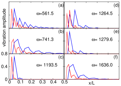
Figure 2: (color online). Normalized vibration amplitudes vs. reduced coordinate $x$ of each carbon atom. From (a) to (f) are six edge modes in (10, 2) graphene strip (blue solid line) and (20, 2) graphene strip (red dotted line). The frequency $\omega$ for each mode given in the figure is in cm^-1.

For a one-dimensional (1D) harmonic chain with a uniform spring constant $K$, the lead self-energy is given by $\Sigma^{r}[\omega]=-K\lambda$, where $\lambda$ satisfies $K\lambda+(\omega+i\eta)^{2}-2K+K/\lambda=0$ and $|\lambda|<1$. Both the real part and imaginary part are smooth functions of the angular frequency $\omega$. However, this is not true in general. For sufficiently complex leads, we find $\delta$-function-like peaks on an otherwise smooth background, see Fig. 1. What is plotted in Fig. 1 is the surface density of states defined according to

$$D_{s}(\omega)=-\frac{2\omega}{\pi}{\rm Im}{\rm Tr}\,g^{r}_{L}[\omega].$$ (10)

The above formula gives the bulk phonon density of states if $g^{r}$ is replaced by the central part Green’s function $G^{r}$. The peaks in Fig. 1 are not numerical artifacts, but real singularities in the semi-infinite lead surface Green’s function or self-energy. If we omit them, the identity (a special case of the Kramers-Kronig relation)

$$\Sigma^{r}[\omega=0]=\int_{-\infty}^{+\infty}\frac{d\omega}{\pi}\frac{{\rm Im}\,\Sigma^{r}[\omega]}{\omega}$$ (11)

will be violated. These sparks are indeed $\delta$ functions. As the small quantity $\eta$ in $(\omega+i\eta)^{2}$ decreases, the peaks become higher and narrower, but the integral in a fixed interval around the peak remains constant. These peaks are not related to the van Hove singularities of bulk system density of states, as the locations of the peaks are not at these associated with zero group velocities. The singularities of the self-energy can be approximated as proportional to

$$\frac{1}{\omega-\omega_{0}+i\eta}\approx P\frac{1}{\omega-\omega_{0}}-i\pi\delta(\omega-\omega_{0}),$$ (12)

where $P$ stands for principle value.

To interpret these peaks, we did a calculation of the vibrational eigenmodes for a finite system. We find localized modes with frequencies matching that of the delta peaks in $D_{s}(\omega)$. We use “General Utility Lattice Program” (GULP)Gale to calculate the phonon modes of graphene strip, with fixed boundary condition in $x$ direction and periodic boundary condition in $y$ direction. These boundary conditions are the same as that in the calculation of lead surface Green’s function. Six localized modes are found in ($n$, 2) graphene strips. Fig. 2 shows the normalized vibrational amplitude of each atom in all six localized modes of (10,2) (blue solid) and (20, 2) graphene strip (red dotted). In these modes the vibrational amplitude decreases exponentially to zero from edge into the center. The frequency of these localized modes are 561.5, 741.3, 1193.5, 1264.5, 1279.6, and 1636.0 cm^-1. These values match very well to that of the delta peaks in $D_{s}(\omega)$ shown in Fig. 1. These frequency values are the same in (10, 2) and (20, 2) graphene strip. After a critical distance $L_{c}$ from the edge, the vibration amplitude decreases to zero. $L_{c}$ is the same in (10, 2) and (20, 2) graphene strip. So these localized modes are relatively more ‘localized’ in longer graphene strip as shown in Fig. 2. Because of their localizing property, these modes are important in thermal transport. There are localized modes both at the edges of leads and edges of center. They have opposite effect on the thermal conductance. (1) Localized modes at the edges of leads are beneficial for thermal conductance. Because in these modes, atoms at the edges of leads have very large vibration amplitude. As a result, thermal energy can transport from leads into center more easily. (2) Localized modes at the edges of the center have negative effect on thermal conductance. In these modes, only outside atoms have large vibrational amplitudes while inside atoms have small vibration amplitudes or even do not vibrate at all. So thermal energy are also localized at the edges, making it difficult to be transported from one end to the other end. The effects of (1) and (2) are such that the net result is equivalent to a perfect periodic system without boundary resistance.

The localized modes are a consequence of dividing the infinite system abruptly and artificially into leads and center. Implementing these delta-peak singularities in a QMD simulation is impossible, since these modes are not decaying in time for the real-time self-energy $\Sigma^{r}(t)$. Thus, we are forced to remove these peaks from the imaginary part of $\Sigma^{r}$, and reconstruct a real part using the Hilbert transform from the imaginary part with the delta peaks removed. The damping kernel for the QMD dynamics is computed from (for $t>0$)

$$\Gamma(t)=-\int_{t}^{+\infty}\!\!\!\!\Sigma^{r}(t^{\prime})dt^{\prime}=\int_{-\infty}^{+\infty}\frac{d\omega}{\pi}\frac{{\rm Im}\Sigma^{r}[\omega]}{-\omega+i\epsilon}e^{-i\omega t-\epsilon t}.$$ (13)

In practice, the removal of the peaks is done by choosing a small $\eta$ $(\approx 10^{-8})$. Since the sampling of $\omega$ is at a finite spacing, typically with about $10^{2}$ points, we almost always miss the peaks if $\eta$ is small.

In calculating the ballistic transmission through Caroli formula, the omission of the delta peaks at a set of points of measure zero has no consequence. However, the existence of the singularities is also reflected through the real part of the self-energy. If the real part uses the Hilbert transformed version with the delta peaks omitted, the transmission coefficient $T[\omega]$ will not be flat steps as expected for a perfect periodic system. Thus, removing the delta peaks consistently means we are using a lead that is modified from the original one.

IV Difference between QMD and NEGF: A Feynman diagrammatic analysis

In this section, we give an analysis of the difference between fully quantum-mechanical NEGF and the quasi-classical generalized Langevin dynamics. A similar result was presented in ref. luwang09, briefly for the case of electron-phonon interaction. The starting point is a formal solution of Eq. (5) with the quasi-classical approximation and a symmetrized correlation matrix for the noise:

$$u(t)=-\int G^{r}(t,t^{\prime})\bigl{[}\xi(t^{\prime})+F_{n}(t^{\prime})\bigr{]}dt^{\prime},$$ (14)

where we have omitted the superscript $C$ on $u$ for simplicity, $G^{r}$ is the retarded Green’s function of the central region for the ballistic system (when $F_{n}=0$). We have also left out a possible term satisfying a homogeneous equation [Eq. (5) when $\xi=F_{n}=0$] and depending on the initial conditions. Physically, such term should be damped out. Provided that the central part is finite, such term should not be there and this is consistent with the fact that the final results are independent of the initial distribution of the central part in steady states.

We consider the expansion of the nonlinear force of the form

$$(F_{n})_{i}=-\sum_{j,k}T_{ijk}u_{j}u_{k}-\sum_{j,k,l}T_{ijkl}u_{j}u_{k}u_{l},$$ (15)

where $T_{ijk}$ and $T_{ijkl}$ are completely symmetric with respect to the permutation of the indices. From repeated substitution of Eq. (14) back into itself, we can see that $u(t)$ is expressed as polynomials of $G^{r}$ and $\xi$. The correlation functions of $u$ can then be calculated using the fact that the noise is gaussian, and Wick’s theorem applies. It is advantageous to define two types of (quasi-classical) Green’s functions, as

$$-\frac{i}{\hbar}\bigl{\langle}u(t)u^{T}(t^{\prime})\bigr{\rangle} \equiv \bar{\mathcal{G}}_{n}(t,t^{\prime})$$ (16)

$$\frac{i}{\hbar}\bigl{\langle}u(t)\xi_{L}^{T}(t^{\prime})\bigr{\rangle} \equiv \int\mathcal{G}_{n}^{r}(t,t^{\prime\prime})\bar{\Sigma}_{L}(t^{\prime\prime},t^{\prime})dt^{\prime\prime}.$$ (17)

The energy current is calculated by the amount of decrease of energy in the left (or right) lead:

$$I_{L}=-\Bigl{\langle}\frac{H_{L}}{dt}\Bigr{\rangle}=-\frac{\partial}{\partial t}\bigl{\langle}{u^{C}(t)}^{T}V^{CL}u^{L}(t^{\prime})\bigr{\rangle}\Big{|}_{t=t^{\prime}=0}.$$ (18)

We can replace $u^{L}$ with the solution, Eq. (3). Going into the Fourier space and some algebraic manipulation, we can write

$$I_{L}=-\int_{-\infty}^{+\infty}\frac{d\omega}{2\pi}\hbar\omega\,{\rm Tr}\bigl{(}\mathcal{G}^{r}_{n}[\omega]\bar{\Sigma}_{L}[\omega]+\bar{\mathcal{G}}_{n}[\omega]\Sigma_{L}^{a}[\omega]\bigr{)},$$ (19)

where the Fourier transform is defined in the usual way, e.g., $\bar{\mathcal{G}}[\omega]=\int_{-\infty}^{+\infty}\bar{\mathcal{G}}(t)e^{i\omega t}dt$. The above equation has the same form as the NEGF one, provided that we can identify the quasi-classical Green’s functions defined in Eq. (16) and (17) with the quantum ones, $\bar{G}=\frac{1}{2}(G^{>}+G^{<})$ and $G^{r}$. [It looks slightly different from the expression of Eq. (5) in ref. wang-wang-zeng-06, , where only $G^{<}$ appears. There is an error in that paper. One should take the real part of that expression, or add its complex conjugate. By doing this, we obtain a symmetrized expression with respect to $G^{<}$ and $G^{>}$.]

Figure 3: The top two lines are for the quasi-classical self-energies $\mathsf{\Sigma}_{n}^{r}$ and $\bar{\mathsf{\Sigma}}_{n}$; the next two lines are the corresponding NEGF results. A line without arrow represents $\bar{G}$. A line with an arrow represents $G^{r}$ when read following the arrow, or $G^{a}$ when read against the direction of arrow. A line with single sided arrow represents $G^{>}$ when following the arrow and $G^{<}$ when read against the sense of arrow.

We compare $\mathcal{G}^{r}_{n}$ and $\bar{\mathcal{G}}_{n}$ with their fully quantum-mechanical counterpart $G^{r}_{n}$ and $\bar{G}_{n}$ through the nonlinear self-energies. It is not known if a Dyson equation for $\mathcal{G}^{r}_{n}$ is still valid in the sense that the self-energy contains only irreducible graphs, but we simply ‘define’ the retarded nonlinear self-energy through

$$\mathsf{\Sigma}_{n}^{r}=\bigl{(}G^{r}\bigr{)}^{-1}-\bigl{(}\mathcal{G}^{r}_{n}\bigr{)}^{-1},$$ (20)

and similarly define $\bar{\mathsf{\Sigma}}_{n}$ by

$$\bar{\mathcal{G}}_{n}=\mathcal{G}^{r}_{n}\left(\bar{\Sigma}+\bar{\mathsf{\Sigma}}_{n}\right)\mathcal{G}^{a}_{n}.$$ (21)

To simplify the representation of the diagrams, we have used the fact that $G_{jl}^{r}(t,t^{\prime})=G_{lj}^{a}(t^{\prime},t)$, $G_{jl}^{>}(t,t^{\prime})=G_{lj}^{<}(t^{\prime},t)$, and the Keldysh relation in frequency domain $\bar{G}=G^{r}\bar{\Sigma}G^{a}$. In Fig. 3 we give the lowest-order diagrams of the two types of self-energies and contrast with the NEGF results. Numerous cross terms involving products of $T_{ijk}$ and $T_{ijkl}$ are not shown. The NEGF results are obtained in ref. WZWG-pre07, (Fig. 3) for the contour ordered version, here we have separated out explicitly for $\Sigma^{r}_{n}$ and $\bar{\Sigma}_{n}=\frac{1}{2}(\Sigma^{>}_{n}+\Sigma^{<}_{n})$. It is clear from Eq. (20) and (21) that, when the nonlinear couplings $T_{ijk}$ and $T_{ijkl}$ are zero, we have $\mathcal{G}^{r}_{n}=G^{r}$ and $\bar{\mathcal{G}}_{n}=\bar{G}$. Thus, for ballistic systems, NEGF and quasi-classical MD agree exactly. To leading order in the non-linear couplings [$O(T_{ijk}^{2})$ and $O(T_{ijkl})$] the retarded nonlinear self-energies agree. The difference starts only at a higher order. The self-energies $\bar{\Sigma}_{n}$ disagree even at the lowest order. The NEGF and quasi-classical diagrams become the same if we take the “classical limit” $\hbar\to 0$ with a new definition of classical Green’s functions $G^{r}\to G^{r}_{{\rm cl}}$ and $\hbar G^{>}\approx\hbar G^{<}\to\bar{G}_{{\rm cl}}$. In this limit, the distinction between $G^{>}$ and $G^{<}$ disappears. The extra diagrams go to zero because they are high orders in $\hbar$.

V Testing runs and comparison with NEGF

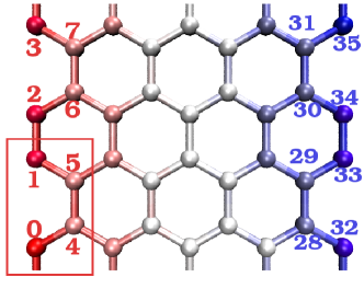
Figure 4: (color online). The structure for an armchair graphene strip with $(n,m)=(4,2)$. The box in red line is the translational period.

Fig. 4 is the configuration of a system in the simulation. There are four atoms in the translational period. A pair of numbers ($n$, $m$) are introduced to denote the number of periods in the horizontal and vertical directions. They should not be confused with the chirality indices of the nanotubes. This figure shows the particular case of armchair graphene strip with ($n$, $m$)=(4, 2). For zigzag configurations, the unit cell is rotated by 90 degrees. In the vertical direction, a periodical boundary condition is applied. In the simulation box, atoms in the left-most columns labelled 0–7 are fixed left lead, atoms in the right-most columns labelled 28–35 are the fixed right lead, and the heat baths are applied to the columns close to them. The temperature of the leads are set according to $T_{L}=T(1+\alpha)$, and $T_{R}=T(1-\alpha)$. The thermal conductance is computed from $\sigma=I_{L}/(T_{L}-T_{R})$.

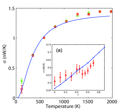
Figure 5: (color online). A comparison of temperature dependence of the thermal conductance for an armchair graphene strip with $(n,m)=(4,2)$, solid line: NEGF, circle: QMD with velocity Verlet, square: QMD with fourth order Runge-Kutta. (a) The $\lambda$ dependence for the same system at 300 K for QMD with velocity Verlet (circle) and NEGF (solid line).

Test runs, shown in Fig. 5, with parameters $\alpha=0.4$, $\lambda=0.6$, $f=1.2$, $K_{\rm onsite}=0.01$ (eV/(Å${}^{2}u$)), and $\epsilon=0.001$ ($10^{14}$ Hz) with the geometry of Fig. 4, demonstrate that QMD implemented by the velocity Verlet and fourth order Runge-Kutta gives the correct results in comparison with ballistic NEGF. For a system of such small sizes, the conductance behaves ballistically. The one implemented by the velocity Verlet agrees very well with the NEGF result in the low-temperature regime. Other implementation methods, like an implicit two-stage fourth order Runge-Kutta, also turn out to give similar results. Thus, the results are rather insensitive to the integration algorithms used. This suggests the success of simulating quantum transport not only for the one-dimensional quartic onsite model wangPRL07 , but also for the large systems. Due to the artificial parameters added in order to overcome the instability, the thermal conductance obtained was slightly higher than the ballistic one in high-temperature regime. We note that the parameters $\lambda$, $f$, and $K_{\rm onsite}$ are incorporated in the NEGF calculation, the effect of $\epsilon$ is not taken care correctly in NEGF. This may explain the discrepancy at high temperatures. We further analyze the $\lambda$ dependence of the thermal conductance for the $(4,2)$ graphene strip: the inset Fig. 5(a) represents the room temperature (300 K) results, where the thermal conductance exhibits linear dependence on $\lambda$. The conductance reduces by about half when $\lambda$ is reduced from 1 to 0. Besides $\lambda$, other parameters also have their own impacts, for instance, smaller $\epsilon$ lowers the effect of the artificial damping, but requires much larger integration domain and therefore brings the risk of truncating the spectrum and providing the wrong self energy. The conductance is independent of $\epsilon$ if it is in the range $0.001$ to $0.02$.

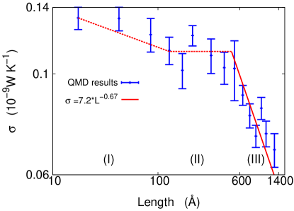
Figure 6: (color online). The dependence of the thermal conductance on the length of the system at $300\,$K in double logarithmic scale. Phonon transport changes gradually from ballistic to diffusive with increasing length of the system.

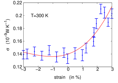
Figure 7: (color online). The effect of strain on the thermal conductance of the graphene. The dotted line (in red) is guide to the eye.

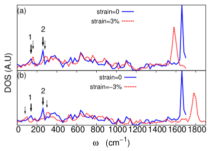
Figure 8: (color online). Phonon density of state (DOS) for graphene under elongation strain (a), and compression strain (b).

VI Results of nanoribbon under tension

In the simulation, typical MD steps are $10^{5}$ of 0.5 fs, which is long enough to obtain converged thermal conductance. The stabilizing factor is $\lambda=0.6$ with an onsite force constant for all the atoms $K_{\rm onsite}=0.01\,$eV/(Ųu), and other parameters $f=1.2$ and $\epsilon=10^{-3}$ $(10^{14}$Hz).

Fig. 6 shows the dependence of the thermal conductance on the length ($L$) of the system for $(n,2)$ zigzag graphene strip at $300\,$K. There are three regions labeled (I), (II) and (III) in the figure respectively for $L$ in [10, 100], [100, 600] and [600, 1400] Å. In the very short length region (I), thermal transport should be in the ballistic regime, where thermal conductance is a constant independent of the length of the system. But here the thermal conductance exhibits decreasing behavior. Actually, this decreasing behavior is mainly attributed to the localized modes at the edge of the center region. As shown in Fig. 2, these modes will be more localized in longer graphene strips. So they make little contribution to the thermal transport in short graphene strips due to their localizing property, and even this little contribution is further reduced with increasing length. That is the reason for the decrease of thermal conductance in this length region. After $L\approx 100\,$Å, these localized modes are fully localized, so they do not contribute to the thermal conductance anymore. In region (II), the thermal transport is in the ballistic regime, where the thermal conductance is more or less a constant. In region (III), this curve decreases as $L$ increases, indicating cross-over to the diffusive thermal transport. This length scale is consistent with previous theoretical results.Mingo Thermal conductance in this region can be fitted by a power function $\sigma=6.1\,L^{-0.66}$ (dotted line). So the thermal conductivity is proportional to the length as $L^{0.34}$. This exponent 0.34 agrees with previous results on nanotubes and other quasi-1D systems.wang-li-PRL04 ; ZhangG ; WangJ

The associated values of thermal conductivity, $\kappa=\sigma L/S$, where $L$ is length and $S$ is cross-section area, is too small. The smallness is attributed to the boundary resistance caused mainly by $\lambda\neq 1$ and the omission of the delta-peak lead self energies. For a perfect 1D system of $(\infty,2)$ the conductance with the Brenner potential is 0.72 nW/K from a ballistic NEGF calculation. If the leads are replaced by those of omitting the delta-peaks as discussed in Sec.III, the NEGF (4,2) system result that is consistent with our simulation setup is reduced to $0.19\,$nW/K. This is quite close to, but still some discrepancy with, QMD result. These may be due to nonlinearity and other unexplained systematic errors.

In Fig. 7, the effect of the strain on the thermal conductance of graphene is displayed for a system of zigzag (4, 2). To mimic the experimental condition,Mohiuddin ; Huang ; Ni the strain is introduced in two steps. Firstly, the strain is generated to the whole graphene system in Fig. 4. Secondly, atoms in the center are fully relaxed with left and right leads fixed. And we then do the MD simulation on this optimized graphene system. We find that the thermal conductance increases with increasing elongation on graphene. But compression on graphene does not change the value of the thermal conductance appreciably.

To understand this strain effect on the thermal conductance, we study the density of state (DOS) of the phonons in Fig. 8. The DOS is calculated from the Brenner empirical potential as implemented in GULP for (4, 2) geometry with fixed boundary conditions in $x$ direction, and periodically extended in $y$ direction. We use GULP to do optimization for the strained graphene with two leads fixed firstly, and then calculate the DOS of this relaxed system. As shown in Fig. 8 (a), the high frequency Raman active mode (G mode) around $1600\,$cm^-1 shows obvious red-shift under extension strain, which agrees with the recent experimental results.Mohiuddin ; Huang Furthermore, Fig. 8 (b) predicts the blue-shift of the G mode with compression strain.

For thermal conductance of the graphene at room temperature, the phonon modes with frequency about $200\,$cm^-1 are important. We can see two significant modes (1 and 2) in this frequency region in Fig. 8. When the graphene is elongated, both modes 1 and 2 are blue-shifted [Fig. 8 (a)], which results in increasing of thermal conductance. However, if the graphene is compressed, modes 1 and 2 shift in opposite directions [shown in Fig. 8 (b)]. As a result, the contribution of these two modes to the thermal conductance cancels with each other. That is the reason for the almost unchanged value of the thermal conductance under compression.

VII Results on nanotubes

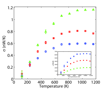
Figure 9: (color online). Temperature dependence of the thermal conductance and thermal conductivity for zigzag carbon nanotubes with $(n,m)=(10,5)$ (triangle), $(30,5)$ (square), and $(60,5)$ (circle).

Fig. 9 shows our simulation results on zigzag carbon nanotubes of chirality (5,0) with different lengths by using the same parameters as that of the previous sections. Each data point typically takes about 48 hours on an AMD Opteron CPU. The thermal conductivity is computed according to $\kappa=\sigma L/S$, where $L$ is the length of the sample, and assuming a cross-section area of $S=12\,$Ų. Both the thermal conductance and thermal conductivity monotonically increase with the temperature in the low-temperature regime, which agrees with the available experimental data and demonstrates the ability of QMD to predict the quantum effect in this regime. This is completely neglected in the classical MD approaches.berber00 ; maruyama02 ; yaozh05 ; ZhangG ; lukes07 For nanotubes with 12.8 nm (30,5) and 25.6 nm (60,5) length, as the temperature increases, the thermal conductance and corresponding thermal conductivity start to drop at 850K, this decrement is consistent with the classical prediction, which indicates that the quantum correction becomes much smaller. Yet, such decline has not been observed in the shorter case with a length of 4.26 nm. This difference shows that a transition from ballistic to diffusive happens when the length gets longer. The thermal conductance decreases but conductivity still increases with nanotubes length; we are still in transition to diffusive regime.WangJ However, the values at high temperatures are comparable to previous MD results.

VIII A critique to the quantum correction method

The quantum correction method was first suggested in refs. czwang90, ; yhlee91, ; jli98, and used by a number of researcherslukes07 ; nyang08 ; mchwu09 ; scwang09 without carefully examining its validity. From the simple kinetic theory of thermal transport coefficient, the thermal conductivity can be written as $\kappa=1/(3V)\sum_{k}c_{k}v_{k}l_{k}$ where $c_{k}$ is the heat capacity of a mode $k$, and $v_{k}$ and $l_{k}$ are the associated phonon group velocity and mean free path, $V$ is the volume of the system. Provided that the phonon velocity $v_{k}$ and mean free path $l_{k}$ of mode $k$ are approximately independent of $k$, we can argue that the quantum conductivity is scaled down by the quantum heat capacity from the classical value. In quantum correction, the temperature is also redefined such that the classical kinetic energy is equated with the corresponding quantum kinetic energy of a harmonic lattice. Here it is not clear whether the zero-point motion should be included or not.yhlee91 ; lukes07 ; maiti97

To a large extent, a constant phonon velocity is a good approximation. However, it is well-known that the phonon mean free path is strongly dependent on the frequencies, e.g., in Klemens’ theory for umklapp processklemens94 , $l\sim\omega^{-2}$. To what extent the quantum correction works is questionable. There is one special case that we can answer this question definitely, although this is for conductance, not conductivity. Let us consider a 1D harmonic chain and compute its conductance exactly and compare it with a classical dynamics with quantum correction. The correct answer for the thermal conductance is given by the Landauer formula,

$$\sigma_{{\rm QM}}=\int_{0}^{\infty}{d\omega\over 2\pi}\hbar\omega\,T[\omega]{\partial f\over\partial T}=\int_{0}^{\omega_{\rm MAX}}\!\!\!\!\!c(\omega){d\omega\over 2\pi},$$ (22)

where the transmission $T[\omega]$ is one for a uniform chain, $\omega_{{\rm MAX}}=\sqrt{4K/m}$ is the maximum frequency for a chain with spring constant $K$ and mass $m$. $c(\omega)=\hbar\omega\partial f/\partial T$ is the heat capacity of the mode at frequency $\omega$. The corresponding classical value is obtained by approximating the Bose distribution function with $f\approx k_{B}T/(\hbar\omega)$. This gives the correct classical value of conductance as

$$\sigma_{\rm CL}=\frac{\omega_{{\rm MAX}}}{2\pi}k_{B}.$$ (23)

Now we consider quantum correction to Eq. (23). The total quantum heat capacity of a 1D harmonic chain is

$$C=\sum_{k}c_{k}=L\int_{0}^{\omega_{\rm MAX}}{c(\omega)\over v(\omega)}{d\omega\over\pi},$$ (24)

where $v(\omega)=d\omega/dk=(a/2)\sqrt{\omega_{\rm MAX}^{2}-\omega^{2}}$ is the phonon group velocity. The classical value is $Nk_{B}=Lk_{B}/a$, $a$ is lattice constant.

According to the quantum correction scheme, the result from a classical dynamics is corrected by multiplying the classical value by the ratio of quantum to classical heat capacity, given

$$\sigma_{\rm CORR}=\sigma_{\rm CL}\frac{C}{Nk_{B}}=\int_{0}^{\omega_{\rm MAX}}\!\frac{a\omega_{\rm MAX}}{\pi v(\omega)}c(\omega){d\omega\over 2\pi}.$$ (25)

This does not agree with the correct quantum result of Eq. (22). There is no need to shift the classical temperature as $\sigma_{\rm CL}$ is independent of the temperature. The heat capacity at frequency $\omega$ is weighted differently in two cases. Even if the group velocity can be approximated by a constant by $v(0)=a\sqrt{K/m}$, valid at very low temperatures, the two results still differ by a factor of $\pi/2$.

IX Conclusion

We have presented a quick derivation of the generalized Langevin equation, emphasizing its connection with NEGF. The inputs to run the Langevin dynamics can be calculated in the standard way from a NEGF phonon transport calculation. The implementation details are given, such as the generation of colored noise vector $\xi$. We found quite generically that the lead self-energies contain delta-function peaks for quasi-one-dimensional systems. These delta peaks represent surface or edge modes. This complicates the molecular dynamics simulations. These delta peaks in the spectra have to be removed in order to obtain a stable simulation. We hope that the instability is specific to the systems of quasi-1D carbon graphene strips or nanotubes. If the leads are modeled as bulk 3D systems, the noise spectra should be more smooth, and should produce a stable dynamics. The quasi-classical approximation which results to the generalized Langevin equation is analyzed using Feynman diagrams and its results are compared with NEGF. It is found that, to lead order, the nonlinear retarded self-energy agrees with NEGF, while $\bar{\Sigma}_{n}$ does not, mainly due to the fact that QMD cannot distinguish between $G^{<}$ and $G^{>}$. As a by-product, we see easily that QMD and NEGF agree for linear systems. QMD also gives the correct classical limit. We presented test runs and compared with NEGF for the thermal conductance. Long $(n,2)$ graphene strips are simulated to study the crossover from ballistic transport towards diffusive transport. Effect of strain is also studied. The results of carbon nanotubes are also presented. Our simulations are one of the first examples of the QMD on realistic systems. Finally, the quantum correction method is critically examined.

References

- (1) D. Frenkel and B. Smit, Understanding Molecular Simulation, 2nd ed., (Academic Press, San Diego, 2001).
- (2) S. Lepri, R. Livi, and A. Politi, Phys. Rep. 377, 1 (2003).
- (3) A. J. H. McGaughey and M. Kaviany, Adv. Heat Transf. 39, 169 (2006).
- (4) J.-S. Wang, Phys. Rev. Lett. 99, 160601 (2007).
- (5) J.-S. Wang, J. Wang, and J. T. Lü, Eur. Phys. J. B, 62, 381 (2008).
- (6) S. A. Adelman and J. D. Doll, J. Chem. Phys. 64, 2375 (1976).
- (7) A Dhar and D. Roy, J. Stat. Phys. 125, 805 (2006).
- (8) G. W. Ford, M. Kac, and P. Mazur, J. Math. Phys. 6, 504 (1965).
- (9) A. Schmid, J. Low Temp. Phys. 49, 609 (1982).
- (10) U. Weiss, Quantum Dissipative Systems, 3rd ed., (World Scientific, Singapore, 2008).
- (11) M. P. Lopez Sancho, J. M. Lopez Sancho, and J. Rubio, J. Phys. F: Met. Phys. 15, 851 (1985).
- (12) G. S. Fishman, Monte Carlo, concepts, algorithms, and applications, p. 223, (Springer, New York, 1996).
- (13) G. H. Golub and C. F. van Loan, Matrix Computations, 3rd ed. p. 143 (Johns Hopkins Univ. Press, Baltimore, 1996).
- (14) D. W. Brenner, O. A. Shenderova, J. A. Harrison, S. J. Stuart, B. Ni, and S. B. Sinnott, J. Phys.:Condens. Matter, 14, 783 (2002).
- (15) D. Janežič and B. Orel, Int. J. quantum Chem. 51, 407 (1994).
- (16) J. D. Gale, JCS Faraday Trans., 93, 629 (1997).
- (17) J. T. Lü and J.-S. Wang, J. Phys.: Condens. Matter, 21, 025503 (2009).
- (18) J.-S. Wang, J. Wang, and N. Zeng, Phys. Rev. B 74, 033408 (2006).
- (19) J.-S. Wang, N. Zeng, J. Wang, and C. K. Gan, Phys. Rev. E 75, 061128 (2007).
- (20) N. Mingo and D. A. Broido, Phys. Rev. Lett 95, 096105 (2005).
- (21) J.-S. Wang and B. Li, Phys. Rev. Lett. 92, 074302 (2004).
- (22) G. Zhang and B. Li, J. Chem. Phys. 123, 114714 (2005).
- (23) J. Wang and J.-S. Wang, Appl. Phys. Lett. 88, 111909 (2006).
- (24) T. M. G. Mohiuddin, A. Lombardo, R. R. Nair, A. Bonetti, G. Savini, R. Jalil, N. Bonini, D. M. Basko, C. Galiotis, N. Marzari, K. S. Novoselov, A. K. Geim, and A. C. Ferrari, Phys. Rev. B 79, 205433 (2009).
- (25) M. Huang, H. Yan, C. Chen, D. Song, T. F. Heinz and J. Hone, arXiv:0812.2258.
- (26) Z. H. Ni, T. Yu, Y. H. Lu, Y. Y. Wang, Y. P. Feng and Z. X. Shen, ACS Nano 2, 2301 (2008).
- (27) S. Berber, Y.-K. Kwon, and D. Tománek, Phys. Rev. Lett. 84, 4613 (2000).
- (28) S. Maruyama, Physica B, 323, 193 (2002).
- (29) Z. Yao, J.-S. Wang, B. Li, and G.-R. Liu, Phys. Rev. B 71, 085417 (2005).
- (30) J. R. Lukes and H. Zhong, J. Heat Transf. 129, 705 (2007).
- (31) C. Z. Wang, C. T. Chan, and K. M. Ho, Phys. Rev. B 42, 11276 (1990).
- (32) Y. H. Lee, R. Biswas, C. M. Soukoulis, C. Z. Wang, C. T. Chan, and K. M. Ho, Phys. Rev. B 43, 6573 (1991).
- (33) J. Li, L. Porter, and S. Yip, J. Nucl. Mat. 255, 139 (1998).
- (34) N. Yang, G. Zhang, and B. Li, Nano Lett. 8, 276 (2008).
- (35) M. C. H. Wu, and J.-Y. Hsu, Nanotechnology, 20, 145401 (2009).
- (36) S.-C. Wang, X.-G. Liang, X.-H. Xu, and T. Ohara, J. Appl. Phys. 105, 014316 (2009).
- (37) A. Maiti, G. D. Mahan, and S. T. Pantelides, Solid State Comm. 102, 517 (1997).
- (38) P. G. Klemens and D. F. Pedraza, Carbon, 32, 735 (1994).