Study of non-collinear parton dynamics in the prompt photon photoproduction at HERA

Skobeltsyn Institute of Nuclear Physics,
Lomonosov Moscow State University,
119991 Moscow, Russia

Abstract

We investigate the prompt photon photoproduction at HERA within the framework of $k_{T}$-factorization QCD approach. Our consideration is based on the off-shell matrix elements for the underlying partonic subprocesses. The unintegrated parton densities in a proton and in a photon are determined using the Kimber-Martin-Ryskin (KMR) prescription. Additionally, we use the CCFM-evolved unintegrated gluon as well as valence and sea quark distributions in a proton. A conservative error analisys is performed. Both inclusive and associated with the hadronic jet production rates are investigated. The theoretical results are compared with the recent experimental data taken by the H1 and ZEUS collaborations. We study also the specific kinematical properties of the photon-jet system which are strongly sensitive to the transverse momentum of incoming partons. Using the KMR scheme, the contribution from the quarks emerging from the earlier steps of the parton evolution is estimated and found to be of 15 – 20% approximately.

PACS number(s): 12.38.-t, 13.85.-t

1 Introduction

The prompt photon production in $ep$ collisions at HERA is subject of intense studies [1–6]. The theoretical and experimental investigations of such processes have provided a direct probe of the hard subprocess dynamics, since produced photons are largely insensitive to the effects of final-state hadronization. Usually photons are called ”prompt” if they are coupled to the interacting quarks. From the theoretical point, these photons in $ep$ collisions can be produced via direct $\gamma q\to\gamma q$ and resolved production mechanisms. In resolved events, the photon emitted by the electron fluctuate into a hadronic state and a gluon and/or a quark of this hadronic fluctuation takes part in the hard interactions. Prompt photon measurements can be used also to constrain the parton densities in the proton and in the photon.

Recently the H1 and ZEUS collaborations have reported data [2–6] on inclusive and associated (with the hadronic jet) prompt photon production at HERA. However, next-to-leading order (NLO) collinear pQCD calculations [7, 8] are $30-40$% below these data, especially in rear pseudo-rapidity (electron direction) region. It was demonstrated [2–5] that the observed disagreement is difficult to explain with conventional theoretical uncertainties connected with scale dependence and parametrizations of the parton densities. The origin of the disagreement has been ascribed to the effect of initial-state soft-gluon radiation. It was shown [3] that observed discrepancy can be reduced by introducing some additional intrinsic transverse momentum $k_{T}$ of the incoming partons. The ZEUS fit to the data gave a $k_{T}$ value of about 1.7 GeV [3]. A similar situation is observed also at Tevatron energies: in order to describe the measured transverse momentum distributions of the photon the Gaussian-like $k_{T}$ spectrum with an average value of $k_{T}\sim 3$ GeV was introduced [9, 10]. Of course, such large partonic $k_{T}$ must have a significant perturbative QCD component.

The transverse momentum of incoming partons naturally occurs in the framework of $k_{T}$-factorization approach of QCD [11]. In this approach, the transverse momentum $k_{T}$ is generated perturbatively in the course of non-collinear parton evolution via the corresponding (usually Balitsky-Fadin-Kuraev-Lipatov (BFKL) [12] or Ciafaloni-Catani-Fiorani-Marchesini (CCFM) [13]) evolution equations. A detailed description of the $k_{T}$-factorization can be found, for example, in reviews [14–16]. As it was demonstrated in the ZEUS paper [4] and in the recent experimental study [6] performed by the H1 collaboration, the $k_{T}$-factorization predictions [17] for prompt photon photoproduction at HERA are in better agreement with the data than the published results of the collinear NLO pQCD calculations [7, 8].

An important component of the first calculations [17] in the framework of $k_{T}$-factorization approach was the unintegrated quark distributions $f_{q}(x,{\mathbf{k}}_{T}^{2},\mu^{2})$ in a proton. These quantities are poorly known since there are theoretical difficulties in obtaining the quark distributions directly from CCFM equation (see also [14–16] and references therein for more information). At present, the unintegrated quark densities are most often used in the framework of KMR [18] approximation only. As a result, the dependence of the $k_{T}$-factorization predictions [17] on the non-collinear evolution scheme has not been investigated. This dependence in general can be significant and it is a special subject of study in the $k_{T}$-factorization approach.

Therefore, in the present paper in addition to the KMR approach we propose a some simplified way to evaluate the unintegrated quark densities $f_{q}(x,{\mathbf{k}}_{T}^{2},\mu^{2})$ within the CCFM dynamics. First we convolute the CCFM-evolved gluon distribution $f_{g}(x,{\mathbf{k}}_{T}^{2},\mu^{2})$ with the usual unregulated leading-order DGLAP splitting function $P_{qg}(z)$ to obtain the unintegrated sea quark densities. Then we add the CCFM-evolved valence quark densities which have been recently evaluated and applied [19] to the jet production at the LHC conditions (in the framework of Monte-Carlo event generator cascade [20]). Of course, in this way we only simulate the last gluon splitting in the full evolution cascade and do not take into account contribution from quarks coming from the earlier steps of the evolution. But it is not evident a priori, whether the last gluon splitting dominates or not. One of the goals of our study is to clarify this point. In order to estimate the contribution from the quarks involved in the earlier steps of the evolution we use the specific properties of the KMR approach [18] which enables us to discriminate between the various components of the quark distributions [21, 22].

We would like to point out that, in contrast with the our previous investigation [17], the present study is based on the off-shell matrix elements of underlying partonic subprocesses, where the virtualities of both incoming gluons and quark are properly taken into account. Numerically, we will investigate the total and differential cross sections of the inclusive and associated jet prompt photon photoproduction and perform a systematic comparison of our predictions with the available H1 and ZEUS data [2–5]. Our additional goal is to study specific kinematical properties of the photon-jet system which are strongly related to the intrinsic partonic $k_{T}$.

The outline of our paper is following. In Section 2 we recall shortly the basic formulas of the $k_{T}$-factorization approach with a brief review of calculation steps. In Section 3 we present the numerical results of our calculations and a discussion. Section 4 contains our conclusions.

2 Theoretical framework

2.1 The subprocesses under consideration

In $ep$ collisions at HERA prompt photons can be produced by one of three mechanisms: a direct production, a single resolved production and via parton-to-photon fragmentation processes [23]. The direct contribution to the $\gamma p\to\gamma+X$ process is the Compton scattering on the quark (antiquark)

$$\gamma(k_{1})+q(k_{2})\to\gamma(p_{\gamma})+q(p^{\prime}),$$

where the particles four-momenta are given in parentheses. It gives the ${\cal O}(\alpha^{2}_{em})$ order contribution to the hadronic cross section. Here $\alpha_{em}$ is Sommerfeld’s fine structure constant. The single resolved subprocesses are

$$q(k_{1})+g(k_{2})\to\gamma(p_{\gamma})+q(p^{\prime}),$$

$$g(k_{1})+q(k_{2})\to\gamma(p_{\gamma})+q(p^{\prime}),$$

$$q(k_{1})+\bar{q}(k_{2})\to\gamma(p_{\gamma})+g(p^{\prime}).$$

Since the parton distributions in a photon at leading-order have a behavior proportional to $\alpha_{em}\ln\mu^{2}/\Lambda_{\rm QCD}^{2}\sim\alpha_{em}/\alpha_{s}$, these subprocesses give also the ${\cal O}(\alpha^{2}_{em})$ contributions and therefore should be taken into account in our analysis.

The calculation of the off-shell matrix elements (1) — (4) is a very straightforward. Here we would like to only mention two technical points. First, in according to the $k_{T}$-factorization prescription [11], the summation over the incoming off-shell gluon polarizations is carried with $\sum\epsilon^{\mu}\epsilon^{\,\nu}={\mathbf{k}}_{T}^{\mu}{\mathbf{k}}_{T}^{\nu}/{\mathbf{k}}_{T}^{2}$, where ${\mathbf{k}}_{T}$ is the gluon transverse momentum. Second, when we calculate the matrix element squared, the spin density matrix for all on-shell spinors is taken in the standard form $u(p)\bar{u}(p)=\hat{p}+m$. In the case of off-shell initial quarks the on-shell spin density matrix has to be replaced with a more complicated expression [24]. To evaluate it, we ”extend” the original diagram and consider the off-shell quark line as internal line in the extended diagram. The ”extended” process looks like follows: the initial on-shell quark with four-momentum $p$ and mass $m_{q}$ radiates a quantum (say, photon or gluon) and becomes an off-shell quark with four-momentum $k$. So, for the extended diagram squared we write:

$$|{\cal M}|^{2}\sim{\rm Sp}\left[{\bar{\cal T}^{\mu}}\,{\hat{k}+m_{q}\over k^{2}-m_{q}^{2}}\,\gamma^{\nu}\,u(p)\bar{u}(p)\,\gamma_{\nu}{\hat{k}+m_{q}\over k^{2}-m_{q}^{2}}\,{\cal T}_{\mu}\right],$$

where ${\cal T}$ is the rest of the original matrix element which remains unchanged. The expression presented between $\bar{\cal T}^{\mu}$ and ${\cal T}_{\mu}$ now plays the role of the off-shell quark spin density matrix. Using the on-shell condition $u(p)\,\bar{u}(p)=\hat{p}+m_{q}$ and performing the Dirac algebra one obtains in the massless limit $m_{q}\to 0$:

$$|{\cal M}|^{2}\sim{1\over(k^{2})^{2}}{\bar{\cal T}^{\mu}}\,\left(2k^{2}\hat{p}-4(p\cdot k)\hat{k}\right)\,{\cal T}_{\mu}.$$

Now we use the Sudakov decomposition $k=xp+k_{T}$ and neglect the second term in the parentheses in (6) in the small-$x$ limit to arrive at

$$|{\cal M}|^{2}\sim{2\over xk^{2}}{\bar{\cal T}^{\mu}}\,x\hat{p}\,{\cal T}_{\,\mu}.$$

(Essentially, we have neglected here the negative light-cone momentum fraction of the incoming quark). The properly normalized off-shell spin density matrix is given by $x\hat{p}$, while the factor $2/xk^{2}$ has to be attributed to the quark distribution function (determining its leading behavior). With this normalization, we successfully recover the on-shell collinear limit when $k$ is collinear with $p$.

2.2 The CCFM and KMR unintegrated parton distributions

As it was mentioned above, in the framework of $k_{T}$-factorization approach one should consider the unintegrated gluon and quark distributions $f_{a}(x,{\mathbf{k}}_{T}^{2},\mu^{2})$ instead of the conventional (collinear) parton densities $a(x,\mu^{2})$. In the KMR approximation, the unintegrated quark and gluon distributions are given by the expressions [18]

$$f_{q}(x,{\mathbf{k}}_{T}^{2},\mu^{2})=T_{q}({\mathbf{k}}_{T}^{2},\mu^{2}){\alpha_{s}({\mathbf{k}}_{T}^{2})\over 2\pi}\times\atop{\displaystyle\times\int\limits_{x}^{1}dz\left[P_{qq}(z){x\over z}q\left({x\over z},{\mathbf{k}}_{T}^{2}\right)\Theta\left(\Delta-z\right)+P_{qg}(z){x\over z}g\left({x\over z},{\mathbf{k}}_{T}^{2}\right)\right],}$$

$$f_{g}(x,{\mathbf{k}}_{T}^{2},\mu^{2})=T_{g}({\mathbf{k}}_{T}^{2},\mu^{2}){\alpha_{s}({\mathbf{k}}_{T}^{2})\over 2\pi}\times\atop{\displaystyle\times\int\limits_{x}^{1}dz\left[\sum_{q}P_{gq}(z){x\over z}q\left({x\over z},{\mathbf{k}}_{T}^{2}\right)+P_{gg}(z){x\over z}g\left({x\over z},{\mathbf{k}}_{T}^{2}\right)\Theta\left(\Delta-z\right)\right],}$$

where $P_{ab}(z)$ are the usual unregulated leading order DGLAP splitting functions, $q(x,\mu^{2})$ and $g(x,\mu^{2})$ are the conventional quark and gluon densities, $T_{q}({\mathbf{k}}_{T}^{2},\mu^{2})$ and $T_{g}({\mathbf{k}}_{T}^{2},\mu^{2})$ are the quark and gluon Sudakov form factors, and the theta function $\Theta(\Delta-z)$ implies the angular-ordering constraint $\Delta=\mu/(\mu+|{\mathbf{k}}_{T}|)$ specifically to the last evolution step to regulate the soft gluon singularities [18].

Another the solution for the unintegrated gluon distributions have been obtained in [25] from the CCFM evolution equation where all input parameters have been fitted to describe the proton structure function $F_{2}(x,Q^{2})$. The proposed gluon densities (namely, sets A0 and B0) have been applied to the number of QCD processes in the framework of the Monte-Carlo generator cascade [20] and in our calculations [21].

In the present paper we will use both these distributions in our calculations. To accomplish the CCFM-evolved gluon densities, one should apply the relevant unintegrated quark distributions. Below we will use the following way to get the $f_{q}(x,{\mathbf{k}}_{T}^{2},\mu^{2})$. The unintegrated valence quark densities $f_{q}^{(v)}(x,{\mathbf{k}}_{T}^{2},\mu^{2})$ have been obtained recently [19] from the numerical solution of the CCFM-like equation. To calculate the contribution of the sea quarks appearing at the last step of the gluon evolution, $f_{q}^{(g)}(x,{\mathbf{k}}_{T}^{2},\mu^{2})$, we convolute the CCFM-evolved unintegrated gluon distribution $f_{g}(x,{\mathbf{k}}_{T}^{2},\mu^{2})$ with the standard leading-order DGLAP splitting function $P_{qg}(z)$:

$$f_{q}^{(g)}(x,{\mathbf{k}}_{T}^{2},\mu^{2})={\alpha_{s}({\mathbf{k}}_{T}^{2})\over 2\pi}\int\limits_{x}^{1}f_{g}(x/z,{\mathbf{k}}_{T}^{2},\mu^{2})P_{qg}(z)\,dz.$$

Note that in the region of small ${\mathbf{k}}_{T}^{2}<q_{0}^{2}$ the scale in the strong coupling constant $\alpha_{s}$ is kept to be fixed at $q_{0}=1$ GeV. To estimate the contribution of the sea quarks coming from the earlier evolution steps, $f_{q}^{(s)}(x,{\mathbf{k}}_{T}^{2},\mu^{2})$, we apply the procedure based on the specific properties of the KMR scheme. Modifying (8) in such a way that only the first term is kept and the second term is omitted and keeping only the sea quark in first term of (8) we remove the valence and $f_{q}^{(g)}(x,{\mathbf{k}}_{T}^{2},\mu^{2})$ quarks from the evolution ladder. In this way only the $f_{q}^{(s)}(x,{\mathbf{k}}_{T}^{2},\mu^{2})$ contribution to the $f_{q}(x,{\mathbf{k}}_{T}^{2},\mu^{2})$ is taken into account.

We would like to point out that the valence quark densities from the CTEQ 6.1 set have been used [19] as the starting distributions to calculate the CCFM-evolved valence quark distributions in a proton. However, the CTEQ collaboration does not provide the quark and gluon distributions in a photon (which are necessary to calculate the resolved photon contributions), and there is no CCFM-evolved unintegrated quark densities in a photon. Therefore everywhere in our numerical analysis below we apply the KMR approximation for the unintegrated parton densities in a photon. Numerically, in (8) and (9) we have tested the standard GRV-94 (LO) [26] and MSTW-2008 (LO) [27] sets of collinear parton densities in a case of proton and the GRV-92 (LO) [28] and CJKL (LO) [29] sets in a case of photon. To compare the different types of evolution, we have performed the numerical integration of the parton densities $f_{a}(x,{\mathbf{k}}_{T}^{2},\mu^{2})$ over transverse momenta ${\mathbf{k}}_{T}^{2}$. In Fig. 1 we show the obtained ”effective” valence quark distributions in a proton as a function of $x$ for different values of $\mu^{2}$, namely $\mu^{2}=2\,{\rm GeV}^{2}$, $\mu^{2}=10\,{\rm GeV}^{2}$ and $\mu^{2}=100\,{\rm GeV}^{2}$. The solid lines correspond to the CCFM-evolved unintegrated (valence) $u$-quark and $d$-quark densities. The dashed and dash-dotted lines correspond to the relevant KMR distributions based on the collinear GRV-94 (LO) and MSTW-2008 (LO) sets, respectively. We have observed some differences in both normalization and shape between the valence quark densities calculated within all these approaches. Below we will study the dependence of our numerical results on the evolution scheme in detail.

2.3 Cross section for the prompt photon production

Main formulas for prompt photon photoproduction have been obtained in our previous paper [17]. Here we only recall some of them. Let $p_{e}$ and $p_{p}$ be the four-momenta of the initial electron and proton. The direct contribution (1) to the $\gamma p\to\gamma+X$ process in the $k_{T}$-factorization approach can be written as

$$\sigma^{\rm(dir)}(\gamma p\to\gamma+X)=\sum_{q}\int{dx_{2}\over x_{2}}f_{q}(x_{2},{\mathbf{k}}_{2T}^{2},\mu^{2})d{\mathbf{k}}_{T}^{2}{d\phi_{2}\over 2\pi}d{\hat{\sigma}}(\gamma q\to\gamma q),$$

where ${\hat{\sigma}}(\gamma q\to\gamma q)$ is the hard subprocess cross section via quark or antiquark having fraction $x_{2}$ of a initial proton longitudinal momentum, non-zero transverse momentum ${\mathbf{k}}_{2T}$ (${\mathbf{k}}_{2T}^{2}=-k_{2T}^{2}\neq 0$) and azimuthal angle $\phi_{2}$. The expression (11) can be easily rewritten in the form

$$\sigma^{\rm(dir)}(\gamma p\to\gamma+X)=\sum_{q}\int{E_{T}^{\gamma}\over 8\pi(x_{2}s)^{2}(1-\alpha)}|\bar{\cal M}(\gamma q\to\gamma q)|^{2}\times\atop\displaystyle\times f_{q}(x_{2},{\mathbf{k}}_{2T}^{2},\mu^{2})dy^{\gamma}dE_{T}^{\gamma}d{\mathbf{k}}_{2T}^{2}{d\phi_{2}\over 2\pi}{d\phi^{\gamma}\over 2\pi},$$

where $|\bar{\cal M}(\gamma q\to\gamma q)|^{2}$ is the hard matrix element squared which depends on the transverse momentum ${\mathbf{k}}_{2T}^{2}$, $s=(k_{1}+p_{p})^{2}$ is the total energy of the subprocess under consideration, $y^{\gamma}$, $E_{T}^{\gamma}$ and $\phi^{\gamma}$ are the rapidity, transverse energy and azimuthal angle of the produced photon in the $\gamma p$ center-of-mass frame, and $\alpha=E_{T}^{\gamma}\exp y^{\gamma}/\sqrt{s}$.

The formula for the resolved contribution to the prompt photon photoproduction in the $k_{T}$-factorization approach can be obtained by the similar way. But one should keep in mind that the convolution in (11) should be made also with the unintegrated parton distributions $f_{a}^{\gamma}(x,{\mathbf{k}}_{T}^{2},\mu^{2})$ in a photon, i.e.

$$d\sigma^{\rm(res)}(\gamma p\to\gamma+X)=\sum_{a,b}\int{dx_{1}\over x_{1}}f_{a}^{\gamma}(x_{1},{\mathbf{k}}_{1T}^{2},\mu^{2})d{\mathbf{k}}_{1T}^{2}{d\phi_{1}\over 2\pi}\times\atop\displaystyle\times\int{dx_{2}\over x_{2}}f_{b}(x_{2},{\mathbf{k}}_{2T}^{2},\mu^{2})d{\mathbf{k}}_{2T}^{2}{d\phi_{2}\over 2\pi}d{\hat{\sigma}}(ab\to\gamma c),$$

where $a,b,c=q$ and/or $g$, ${\hat{\sigma}}(ab\to\gamma c)$ is the cross section of the photon production in the corresponding parton-parton interaction (2) — (4). Here parton $a$ has fraction $x_{1}$ of a initial photon longitudinal momentum, non-zero transverse momentum ${\mathbf{k}}_{1T}$ (${\mathbf{k}}_{1T}^{2}=-k_{1T}^{2}\neq 0$) and azimuthal angle $\phi_{1}$. We can easily obtain the final expression from equation (13). It has the form

$$\sigma^{\rm(res)}(\gamma p\to\gamma+X)=\sum_{a,b}\int{E_{T}^{\gamma}\over 8\pi(x_{1}x_{2}s)^{2}}|\bar{\cal M}(ab\to\gamma c)|^{2}\times\atop\displaystyle\times f_{a}^{\gamma}(x_{1},{\mathbf{k}}_{1T}^{2},\mu^{2})f_{b}(x_{2},{\mathbf{k}}_{2T}^{2},\mu^{2})d{\mathbf{k}}_{1T}^{2}d{\mathbf{k}}_{2T}^{2}dE_{T}^{\gamma}dy^{\gamma}dy^{c}{d\phi_{1}\over 2\pi}{d\phi_{2}\over 2\pi}{d\phi^{\gamma}\over 2\pi},$$

where $y^{c}$ is the rapidity of the parton $c$ in the $\gamma p$ center-of-mass frame. It is important that the hard matrix elements squared $|\bar{\cal M}(ab\to\gamma c)|^{2}$ depend on the transverse momenta ${\mathbf{k}}_{1T}^{2}$ and ${\mathbf{k}}_{2T}^{2}$. We would like to note that if we average the expressions (12) and (14) over $\phi_{1}$ and $\phi_{2}$ and take the limit ${\mathbf{k}}_{1T}^{2}\to 0$ and ${\mathbf{k}}_{2T}^{2}\to 0$, then we obtain well-known expressions for the prompt photon production in leading-order (LO) perturbative QCD.

The experimental data [2–5] taken by the H1 and ZEUS collaborations refer to prompt photon production in the $ep$ collisions, where the electron is scattered at small angle and the mediating photon is almost real ($Q^{2}\sim 0$). Therefore the $\gamma p$ cross sections (12) and (14) need to be weighted with the photon flux in the electron:

$$d\sigma(ep\to e^{\prime}+\gamma+X)=\int f_{\gamma/e}(y)d\sigma(\gamma p\to\gamma+X)dy,$$

where $y$ is a fraction of the initial electron energy taken by the photon in the laboratory frame, and we use the Weizacker-Williams approximation for the bremsstrahlung photon distribution from an electron:

$$f_{\gamma/e}(y)={\alpha_{em}\over 2\pi}\left({1+(1-y)^{2}\over y}\ln{Q^{2}_{\rm max}\over Q^{2}_{\rm min}}+2m_{e}^{2}y\left({1\over Q^{2}_{\rm max}}-{1\over Q^{2}_{\rm min}}\right)\right).$$

Here $m_{e}$ is the electron mass, $Q^{2}_{\rm min}=m_{e}^{2}y^{2}/(1-y)^{2}$ and $Q^{2}_{\rm max}=1\,{\rm GeV}^{2}$, which is a typical value for the photoproduction measurements at HERA.

The multidimensional integration in (12), (14) and (15) has been performed by means of the Monte Carlo technique, using the routine vegas [30]. The full C$++$ code is available from the authors on request.

2.4 Fragmentation contributions and isolation

In order to reduce the huge background from the secondary photons produced by the decays of $\pi^{0}$, $\eta$ and $\omega$ mesons the isolation criterion is introduced in the experimental analyses. This criterion is the following. A photon is isolated if the amount of hadronic transverse energy $E_{T}^{\rm had}$, deposited inside a cone with aperture $R$ centered around the photon direction in the pseudo-rapidity and azimuthal angle plane, is smaller than some value $E_{T}^{\rm max}$:

$$E_{T}^{\rm had}\leq E_{T}^{\rm max},\atop\displaystyle(\eta-\eta^{\gamma})^{2}+(\phi-\phi^{\gamma})^{2}\leq R^{2}.$$

The both H1 and ZEUS collaborations take $R=1$, $E_{T}^{\rm max}=\epsilon E_{T}^{\gamma}$ with $\epsilon=0.1$ in the experiments [2–5]. The isolation criteria not only reduces the background but also significantly reduces the fragmentation components. It was shown [7, 8] that after applying the isolation cut the contribution from the fragmentation subprocesses is only about 5 or 6% of the total prompt photon cross section. Therefore in our further analysis we will neglect the small fragmentation contribution and consider only the direct and resolved production mechanisms.

3 Numerical results

We now are in a position to present our numerical results. First we describe our theoretical input and the kinematical conditions. After we fixed the unintegrated parton distributions in a proton and in a photon, the cross sections (12) and (14) depend on the energy scale $\mu$. As it often done [7, 8] for prompt photon production, we choose the renormalization and factorization scales to be $\mu=\xi E_{T}^{\gamma}$. In order to estimate the scale uncertainties of our calculations we will vary the parameter $\xi$ between 1/2 and 2 about the default value $\xi=1$. We use LO formula for the strong coupling constant $\alpha_{s}(\mu^{2})$ with $n_{f}=4$ massless quark flavours and $\Lambda_{\rm QCD}=200$ MeV, such that $\alpha_{s}(M_{Z}^{2})=0.1232$.

3.1 Inclusive prompt photon photoproduction

Experimental data for the inclusive prompt photon production at HERA come from both the ZEUS and H1 collaborations. Two differential cross section are determined: first as a function of the transverse energy $E_{T}^{\gamma}$, and second as a function of pseudo-rapidity $\eta^{\gamma}$. The ZEUS data [2] refer to the kinematic region defined by $E_{T}^{\gamma}>5$ GeV and $-0.7<\eta^{\gamma}<0.9$ with electron energy $E_{e}=27.5$ GeV and proton energy $E_{p}=820$ GeV. The fraction $y$ of the electron energy trasferred to the photon is restricted to the range $0.2<y<0.9$. Additionally the available ZEUS data for the prompt photon pseudo-rapidity distributions have been given also for three subdivisons of the $y$ range, namely $0.2<y<0.32$ ($134<W<170$ GeV), $0.32<y<0.5$ ($170<W<212$ GeV) and $0.5<y<0.9$ ($212<W<285$ GeV). The more recent H1 data [5] refer to the kinematic region defined by $5<E_{T}^{\gamma}<10$ GeV, $-1<\eta^{\gamma}<0.9$ and $0.2<y<0.7$ with electron energy $E_{e}=27.6$ GeV and proton energy $E_{p}=920$ GeV.

The transverse energy and pseudo-rapidity distributions of the inclusive prompt photon production for different kinematical regions are shown in Figs. 2 — 4 in comparison with the available HERA data [2, 5]. The solid histograms correspond to the results obtained using the KMR approximation for the unintegrated quark and gluon densities in a proton and in a photon (supplemented with the GRV-94 and GRV-92 parametrizations, respectively). The dashed and dash-dotted histograms correspond to the results obtained with the CCFM-evolved unintegrated quark $f_{q}^{(v)}(x,{\mathbf{k}}_{T}^{2},\mu^{2})$, $f_{q}^{(g)}(x,{\mathbf{k}}_{T}^{2},\mu^{2})$ and gluon $f_{g}(x,{\mathbf{k}}_{T}^{2},\mu^{2})$ distributions in a proton, as it was described in Section 2.2. These calculations are based on the CCFM set A0 and set B0 gluon densities. The numerical predictions have been obtained by fixing both the factorization and normalization scales at the default value $\mu=E_{T}^{\gamma}$. One can see that the H1 and ZEUS data [2, 5] can be reasonably well described by using the KMR unintegrated parton densities. This is in a full agreement with our previous observations [17]. Our predictions tend even to slightly overshoot the ZEUS data at high values of $y$ variable and large photon pseudo-rapidity $\eta^{\gamma}$ (see Fig. 4). Concerning the CCFM predictions, the results coming from the CCFM and KMR parton densities are very similar to each other in the forward region, $\eta^{\gamma}>0.4$. However, we find the some underestimation of the HERA data in the rear pseudo-rapidity $\eta^{\gamma}$ region. One of the possible reasons of such disagreement can be connected with the contributions from the sea quarks involved in the earlier steps of the evolution cascade (below we will refer to these contributions as to ”reduced sea” component). Since the ”reduced sea” is not taken into account in the CCFM evolution we use the properties of the KMR approach to perform a rough numerical estimation of this contribution (see Table 1 and 2), as it was described above in Section 2.2. We found that the ”reduced sea” component gives approximately 15% contribution to the calculated cross sections. However, to avoid double counting we do not sum the CCFM predictions and the estimated ”reduced sea” contributions since part of them can be already included into the CCFM results (via initial parton distributions which enter to the CCFM equation).

uPDF (proton) + uPDF (photon)	$\sigma$ (H1 region) [pb]	$\sigma$ (ZEUS region) [pb]
KMR (GRV-94) + KMRγ(GRV-92)	$45.76^{+4.02}_{-4.48}$	$47.19^{+4.86}_{-4.96}$
KMR (MSTW) + KMRγ(CJKL)	$36.58^{+1.71}_{-2.38}$	$37.97^{+2.13}_{-2.53}$
CCFM (set A0) + KMRγ(GRV-92)	$38.03^{+3.97}_{-2.15}$	$41.20^{+2.97}_{-1.07}$
CCFM (set A0) + KMRγ(CJKL)	$33.48^{+4.41}_{-2.74}$	$36.11^{+3.59}_{-1.99}$
CCFM (set B0) + KMRγ(GRV-92)	$33.40^{+4.07}_{-2.21}$	$36.12^{+3.14}_{-1.26}$
CCFM (set B0) + KMRγ(CJKL)	$29.37^{+4.12}_{-2.63}$	$31.88^{+3.42}_{-1.92}$
”reduced sea”	$7.56$	$7.99$

Table 1: The total cross section of inclusive prompt photon photoproduction obtained in the kinematic range of the H1 and ZEUS experiments. The theoretical uncertainties in the predictions correspond to the usual scale variations, as it was described in the text.

The total cross sections of the inclusive prompt photon production are listed in Table 1. To study the dependence of our results on the evolution scheme we vary the unintegrated parton densities both in a proton and in a photon, as it was described in Section 2.2. Additionally we study the effect of scale variations in the calculated cross sections. We found that this effect is rather large: the relative difference between results for $\mu=E_{T}^{\gamma}$ and results for $\mu=E_{T}^{\gamma}/2$ or $\mu=2E_{T}^{\gamma}$ is about 10%. In the kinematic region of the ZEUS experiment our numerical predictions obtained with the KMR parton densities are rather close to the ones coming from the usual (based on the collinear factorization of QCD) NLO calculations [7, 8].

3.2 Prompt photon photoproduction in association with jet

To calculate the semi-inclusive prompt photon production rates we apply the procedure which has been used previously in [17]. The produced photon is accompanied by a number of partons radiated in the course of the parton evolution. As it has been noted in [31], on the average the parton transverse momentum decreases from the hard interaction box towards the proton. As an approximation, we assume that the parton $k^{\prime}$ emitted in the last evolution step compensates the whole transverse momentum of the parton participating in the hard subprocess, i.e. ${\mathbf{k}^{\prime}}_{T}\simeq-{\mathbf{k}}_{T}$. All the other emitted partons are collected together in the proton remnant, which is assumed to carry only a negligible transverse momentum compared to ${\mathbf{k}^{\prime}}_{T}$. This parton gives rise to a final hadron jet with $E_{T}^{\rm jet}=|{\mathbf{k}^{\prime}}_{T}|$ in addition to the jet produced in the hard subprocess. From these hadron jets we choose the one carrying the largest transverse energy, and then compute the cross section of prompt photon with an associated jets.

The experimental data for this process were obtained by the H1 and ZEUS collaborations. The H1 collaboration presented the cross sections [5] measured differentially as a function of $E_{T}^{\gamma}$, $E_{T}^{\rm jet}$, and the pseudo-rapidities $\eta^{\gamma}$ and $\eta^{\rm jet}$ in the kinematic region defined by $5<E_{T}^{\gamma}<10$ GeV, $E_{T}^{\rm jet}>4.5$ GeV, $-1<\eta^{\gamma}<0.9$, $-1<\eta^{\rm jet}<2.3$ and $0.2<y<0.7$ with electron energy $E_{e}=27.6$ GeV and proton energy $E_{p}=920$ GeV. The more recent ZEUS data [4] refer to the kinematic region defined by $5<E_{T}^{\gamma}<16$ GeV, $6<E_{T}^{\rm jet}<17$ GeV, $-0.74<\eta^{\gamma}<1.1$, $-1.6<\eta^{\rm jet}<2.4$ and $0.2<y<0.8$ with the same electron and proton energies.

The results of our calculations are shown in Figs. 5 — 8 in comparison with the HERA data. One can see that the situation is very similar to the inclusive production case. The dstributions measured by the H1 collaboration are reasonably well reproduced by our calculations supplemented with the KMR unintegrated parton densities. However, there is some discrepancy between the predictions and the ZEUS data. It seems that the origin of this disagreement is connected with the lowest bin in the $E_{T}^{\gamma}$ distribution, where our theoretical results are about 2 times below the ZEUS measurements (see Fig. 5, right panel). In order to investigate it in more detail, we have repeted the calculations with an additional cut on the photon transverse energy, namely $E_{T}^{\gamma}>7$ GeV (keeping the other cuts the same as before). Our results compared to the ZEUS data are shown in Fig. 9. We found a perfect agreement between the theoretical predictions (based on the KMR parton densities) and the data after applying this additional cut (see also [4]). Note that the KMR-based results agree with the H1 measurements [5] in a whole $E_{T}^{\gamma}$ range.

Concerning the CCFM predictions, we found again that they are below the HERA data. In our opinion, it is connected with the missing ”reduced sea” component (which gives about 20% contribution to the total $\gamma$ + jet cross section, see Table 2). Note also that the shape of all predicted pseudo-rapidity $\eta^{\rm jet}$ distributions (based on the CCFM as well as on the KMR unintegrated parton densities) coincide with the ones calculated in the collinear NLO pQCD approximation [7, 8]. As it was pointed out [5], the shape of this distribution is not reproduced well by the LO pQCD calculations. This fact demonstrates that the main part of the collinear high-order corrections is already included at LO level in $k_{T}$-factorization formalism (see also [14–16] for more information).

Now we turn to the total cross section of the prompt photon and associated jet photoproduction at HERA. Results of our calculations within the framework of the $k_{T}$-factorization approach compared to the ZEUS experimental data [4] are listed in Table 2. Similar to the inclusive photon production case, in these calculations we study the dependence of the predicted cross sections on the evolution scheme and the relative effects of scale variations. The measured cross sections are described reasonably well using the $k_{T}$-factorization approach and the KMR-constructed unintegrated parton densities.

Source	$\sigma(\gamma+{\rm jet})$ [pb] (region I)	$\sigma(\gamma+{\rm jet})$ [pb] (region II)
ZEUS measurement [4]	$33.1\pm 3.0~{}{\rm(stat.)}^{+4.6}_{-4.2}~{}{\rm(syst.)}$	$13.8\pm 1.2~{}{\rm(stat.)}^{+1.8}_{-1.6}~{}{\rm(syst.)}$
NLO QCD [7]	$23.3^{+1.9}_{-1.7}$	$14.9^{+1.3}_{-1.0}$
NLO QCD [8]	$23.5^{+1.7}_{-1.6}$	$13.4^{+1.1}_{-0.9}$
KMR (GRV-94) + KMRγ(GRV-92)	$23.10^{+2.46}_{-2.19}$	$14.88^{+1.37}_{-1.17}$
KMR (MSTW) + KMRγ(CJKL)	$19.28^{+1.75}_{-0.89}$	$12.9^{+0.38}_{-0.44}$
CCFM (set A0) + KMRγ(GRV-92)	$17.13^{+1.22}_{-1.22}$	$11.11^{+0.70}_{-0.49}$
CCFM (set A0) + KMRγ(CJKL)	$15.29^{+0.68}_{-1.05}$	$10.06^{+0.45}_{-0.46}$
CCFM (set B0) + KMRγ(GRV-92)	$15.68^{+1.01}_{-0.68}$	$10.26^{+0.55}_{-0.10}$
CCFM (set B0) + KMRγ(CJKL)	$13.85^{+0.81}_{-0.82}$	$9.10^{+0.58}_{-0.40}$
”reduced sea”	$4.49$	$3.11$

Table 2: The total cross section of prompt photon and associated jet photoproduction obtained in the kinematic range $Q^{2}<1$ GeV², $5<E_{T}^{\gamma}<16$ GeV, $6<E_{T}^{\rm jet}<17$ GeV, $-0.74<\eta^{\gamma}<1.1$, $-1.6<\eta^{\rm jet}<2.4$ and $0.2<y<0.8$ (region I). An additional cut $E_{T}^{\gamma}>7$ GeV is applied in the region II.

The most important variables for testing the structure of colliding proton and photon are the longitudinal fractional momenta of partons in these particles. In order to reconstruct the momentum fractions of the initial partons from measured quantities the observables $x_{\gamma}^{\rm obs}$ and $x_{p}^{\rm obs}$ are introduced in the ZEUS analysis [3, 4]:

$$x_{\gamma}^{\rm obs}={E_{T}^{\gamma}e^{-\eta^{\gamma}}+E_{T}^{\rm jet}e^{-\eta^{\rm jet}}\over 2yE_{e}},\quad\displaystyle x_{p}^{\rm obs}={E_{T}^{\gamma}e^{\eta^{\gamma}}+E_{T}^{\rm jet}e^{\eta^{\rm jet}}\over 2E_{p}}.$$

The $x_{\gamma}^{\rm obs}$ distribution is particularly sensitive to the photon structure function. It is known that at large $x_{\gamma}^{\rm obs}$ region ($x_{\gamma}^{\rm obs}>0.85$) the cross section is dominated by the contribution of processes with direct initial photons, whereas at $x_{\gamma}^{\rm obs}<0.85$ the resolved photon contributions dominate [4, 5]. Instead of using the $x_{\gamma}^{\rm obs}$ and $x_{p}^{\rm obs}$ variables, the H1 collaboration refers [5] to $x_{\gamma}^{\rm LO}$ and $x_{p}^{\rm LO}$ observables given by

$$x_{\gamma}^{\rm LO}={E_{T}^{\gamma}(e^{-\eta^{\gamma}}+e^{-\eta^{\rm jet}})\over 2yE_{e}},\quad\displaystyle x_{p}^{\rm LO}={E_{T}^{\gamma}(e^{\eta^{\gamma}}+e^{\eta^{\rm jet}})\over 2E_{p}}.$$

It was argued [5] that these quantities make explicit use only of the photon energy, which is better measured than the jet energy. Our predictions for all these observables compared to the H1 and ZEUS data [4, 5] are shown in Figs. 10 and 11. We conclude again that KMR predictions reasonable agree with the HERA data for both direct and resolved production mechanisms. The sizeble contribition from the ”reduced sea” quarks appears only for the direct production and practically negligible for the resolved one.

Further understanding of the process dynamics and in particular of the high-order correction effects may be obtained from the transverse correlation between the produced prompt photon and the jet. Specially the H1 and ZEUS collaborations have measured [3–5] the distribution on the component of the prompt photon’s momentum perpendicular to the jet direction in the transverse plane, i.e.

$$p_{\perp}=|{\mathbf{p}}_{T}^{\gamma}\times{\mathbf{p}}_{T}^{\rm jet}|/|{\mathbf{p}}_{T}^{\rm jet}|=E_{T}^{\gamma}\sin\Delta\phi,$$

where $\Delta\phi$ is the difference in azimuth between the photon and the accompanying jet. The ZEUS collaboration have measured [3] also the distribution on the $\Delta\phi$ angle. In the collinear leading-order approximation, these distributions must be simply delta functions $\delta(p_{\perp})$ and $\delta(\phi-\pi)$, since the produced photon and the jet are back-to-back in the transverse plane. Taking into account the non-vanishing initial parton transverse momentum leads to the violation of this back-to-back kinematics in the $k_{T}$-factorization approach. The normalised $p_{\perp}$ and $\Delta\phi$ distributions compared to the H1 and ZEUS data [3–5] are shown in Figs. 12 and 13 separately for the regions $x_{\gamma}^{\rm LO}<0.85$ and $x_{\gamma}^{\rm LO}>0.85$ (in the case of ZEUS measurements for $x_{\gamma}^{\rm obs}>0.9$ only). One can see that both the CCFM and KMR predictions are consistent with the data for all $p_{\perp}$ values at $x_{\gamma}^{\rm LO}>0.85$ (or $x_{\gamma}^{\rm obs}>0.9$) and tend to underestimate the data in the large $p_{\perp}$ region at $x_{\gamma}^{\rm LO}<0.85$. However, this underestimation is not significant and therefore we can conclude that the CCFM-evolved parton densities reasonably well simulates the intrinsic partonic $k_{T}$. The $k_{T}$-factorization predictions depicted in Fig. 11 are very similar to the ones [7] obtained in the collinear factorization of QCD at NLO level. The NLO calculations performed by another group [8] give a better description of the $p_{\perp}$ distributions at $x_{\gamma}^{\rm LO}<0.85$ than the ones [7] since in this kinematical region the cross section is dominated by ${\cal O}(\alpha_{s})$ corrections to the processes with resolved photons, which are not included in the calculations [7].

As a final point, we should mention that the corrections for hadronisation and multiple interactions have been taken into account in the NLO analysis of the available HERA data [2–5] performed in the framework of collinear factorization of QCD. The correction factors are typically 0.8 — 1.2 depending on a bin. These corrections are not taken into account in our consideration.

4 Conclusions

In the present paper the evaluated CCFM and KMR unintegrated quark and gluon densities have been applied to the analysis of the recent experimental data on the prompt photon photoproduction taken by the H1 and ZEUS collaborations at HERA. Our consideration is based on the off-shell matrix elements of underlying partonic subprocesses (where the transverse momenta of both quarks and gluons are properly taken into account) and covers both inclusive and associated with the hadronic jet production rates. We have studied the dependences of our numerical results on the evolution scheme and on the standard scale variations. To evaluate the unintegrated quark densities within the CCFM dynamics we have calculated separately the contribution of valence quarks, sea quarks appearing at the last step of the gluon evolution and sea quarks coming from the earlier gluon splittings. In first time the contribution from the last gluon splitting has been calculated as a convolution of the CCFM-evolved unintegrated gluon distribution with the standard leading-order DGLAP splitting function $P_{qg}(z)$. The contribution from the sea quarks involved into the earlier evolution steps has been estimated in the framework of the KMR approximation.

We have found a reasonable agreement between our predictions and the available data. The contributions to the total photon cross section from the quarks emerging from the earlier steps of the parton evolution rather than from the last gluon splitting are estimated to be of 15 – 20% approximately. Additionally we have studied the specific kinematical properties of the photon-jet system which are strongly sensitive to the transverse momentum of incoming partons. We have demonstrated that the $k_{T}$-factorization approach supplemented with the CCFM and KMR parton dynamics reasonably well simulates the intrinsic partonic $k_{T}$.

Note that in our analysis we neglect the contribution from the fragmentation processes and from the direct box diagram ($\gamma g\to\gamma g$). As it was claimed in [7], the direct box diagram, which is formally of the next-to-next-to-leading order, gives approximately 6% contribution to the total NLO cross section. The problem of taking into account the contribution of box diagrams with initial off-shell gluons in the framework of $k_{T}$-factorization is still open.

Figure 1: The effective (${\mathbf{k}}_{T}^{2}$-integrated) valence quark distributions in a proton as a function of $x$ for different values of $\mu^{2}$. The solid lines correspond to the CCFM-evolved quark distributions. The dashed and dash-dotted lines correspond to the KMR predictions based on the collinear GRV-94 (LO) and MSTW-2008 (LO) sets, respectively.

Figure 2: The differential cross sections $d\sigma/dE_{T}^{\gamma}$ for the inclusive prompt photon photoproduction at HERA. The solid histograms correspond to the results obtained using the KMR quark and gluon densities in a proton and in a photon. The dashed and dash-dotted histograms correspond to the results obtained with the CCFM-evolved quark $f_{q}^{(v)}(x,{\mathbf{k}}_{T}^{2},\mu^{2})$, $f_{q}^{(g)}(x,{\mathbf{k}}_{T}^{2},\mu^{2})$ and gluon $f_{g}(x,{\mathbf{k}}_{T}^{2},\mu^{2})$ distributions in a proton. In these calculations we use CCFM set A0 and set B0 gluons, respectively. The experimental data are from H1 [5] and ZEUS [2].

Figure 3: The differential cross sections $d\sigma/d\eta^{\gamma}$ for the inclusive prompt photon photoproduction at HERA. Notation of all histograms is the same as in Figure 2. The experimental data are from H1 [5] and ZEUS [2].

Figure 4: The differential cross sections $d\sigma/d\eta^{\gamma}$ for the inclusive prompt photon photoproduction at HERA calculated in the different kinematical regions. Notation of all histograms is the same as in Figure 2. The experimental data are ZEUS [2].

Figure 5: The differential cross sections $d\sigma/dE_{T}^{\gamma}$ for the prompt photon + jet production at HERA. Notation of all histograms is the same as in Figure 2. The experimental data are from H1 [5] and ZEUS [4].

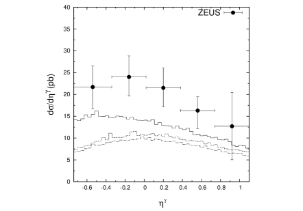
Figure 6: The differential cross sections $d\sigma/d\eta^{\gamma}$ for the prompt photon + jet production at HERA. Notation of all histograms is the same as in Figure 2. The experimental data are from H1 [5] and ZEUS [4].

Figure 7: The differential cross sections $d\sigma/dE_{T}^{\rm jet}$ for the prompt photon + jet production at HERA. Notation of all histograms is the same as in Figure 2. The experimental data are from H1 [5] and ZEUS [4].

Figure 8: The differential cross sections $d\sigma/d\eta^{\rm jet}$ for the prompt photon + jet production at HERA. Notation of all histograms is the same as in Figure 2. The experimental data are from H1 [5] and ZEUS [4].

Figure 9: The differential cross sections $d\sigma/d\eta^{\gamma}$, $d\sigma/d\eta^{\rm jet}$ and $d\sigma/dE_{T}^{\rm jet}$ for the prompt photon + jet production at HERA. The additional cut $E_{T}^{\gamma}>7$ GeV has been applied. Notation of all histograms is the same as in Figure 2. The experimental data are from ZEUS [4].

Figure 10: The differential cross sections $d\sigma/dx_{\gamma}^{\rm LO}$ and $d\sigma/dx_{p}^{\rm LO}$ for the prompt photon + jet production at HERA. Notation of all histograms is the same as in Figure 2. The experimental data are from H1 [5].

Figure 11: The differential cross sections $d\sigma/dx_{\gamma}^{\rm obs}$ for the prompt photon + jet production at HERA. Notation of all histograms is the same as in Figure 2. The additional cut $E_{T}^{\gamma}>7$ GeV has been applied on the right panel. The experimental data are from ZEUS [4].

Figure 12: The normalized differential cross sections $1/\sigma\,d\sigma/dp_{\perp}$ for the prompt photon + jet production at HERA. Notation of all histograms is the same as in Figure 2. The experimental data are from H1 [5].

Figure 13: The normalized differential cross sections $1/\sigma\,d\sigma/dp_{\perp}$ and $1/\sigma\,d\sigma/d\Delta\phi$ for the prompt photon + jet production at HERA. Notation of all histograms is the same as in Figure 1. The experimental data are from ZEUS [3].

References

- [1] J. Breitweg et al. (ZEUS Collaboration), Phys. Lett. B413, 201 (1997).
- [2] J. Breitweg et al. (ZEUS Collaboration), Phys. Lett. B 472, 175 (2000).
- [3] S. Chekanov et al. (ZEUS Collaboration), Phys. Lett. B 511, 19 (2001).
- [4] S. Chekanov et al. (ZEUS Collaboration), Eur. Phys. J. C 49, 511 (2007).
- [5] A. Aktas et al. (H1 Collaboration), Eur. Phys. J. C 38, 437 (2005).
- [6] F.D. Aaron et al. (H1 Collaboration), arXiv:0910.5631 [hep-ex].
- [7] A. Zembrzuski and M. Krawczyk, Phys. Rev. D 64, 114017 (2001).
- [8] M. Fontannaz, J.Ph. Guillet, and G. Heinrich, Eur. Phys. J. C 21, 303 (2001).
- [9] L. Apanasevich, C. Balazs, C. Bromberg et al., Phys. Rev. D 59, 074007 (1999).
- [10] A. Kumar, K. Ranjan, M.K. Jha et al., Phys. Rev. D 68, 014017 (2003).
-
[11]
L.V. Gribov, E.M. Levin, and M.G. Ryskin, Phys. Rep. 100, 1 (1983);
E.M. Levin, M.G. Ryskin, Yu.M. Shabelsky and A.G. Shuvaev, Sov. J. Nucl. Phys. 53, 657 (1991);
S. Catani, M. Ciafoloni and F. Hautmann, Nucl. Phys. B 366, 135 (1991);
J.C. Collins and R.K. Ellis, Nucl. Phys. B 360, 3 (1991). -
[12]
E.A. Kuraev, L.N. Lipatov and V.S. Fadin, Sov. Phys. JETP 44, 443 (1976);
E.A. Kuraev, L.N. Lipatov and V.S. Fadin, Sov. Phys. JETP 45, 199 (1977);
I.I. Balitsky and L.N. Lipatov, Sov. J. Nucl. Phys. 28, 822 (1978). -
[13]
M. Ciafaloni, Nucl. Phys. B 296, 49 (1988);
S. Catani, F. Fiorani and G. Marchesini, Phys. Lett. B 234, 339 (1990);
S. Catani, F. Fiorani and G. Marchesini, Nucl. Phys. B 336, 18 (1990);
G. Marchesini, Nucl. Phys. B 445, 49 (1995). - [14] B. Andersson et al. (Small- Collaboration), Eur. Phys. J. C 25, 77 (2002).
- [15] J. Andersen et al. (Small- Collaboration), Eur. Phys. J. C 35, 67 (2004).
- [16] J. Andersen et al. (Small- Collaboration), Eur. Phys. J. C 48, 53 (2006).
- [17] A.V. Lipatov and N.P. Zotov, Phys. Rev. D 72, 054002 (2005).
-
[18]
M.A. Kimber, A.D. Martin, and M.G. Ryskin, Phys. Rev. D 63, 114027 (2001);
G. Watt, A.D. Martin, and M.G. Ryskin, Eur. Phys. J. C 31, 73 (2003). - [19] M. Deak, H. Jung, and K. Kutak, talk presented at 16th International Workshop on Deep Inelastic Scattering and Related Subjects, 7 — 11 April 2008, University College London, UK.
-
[20]
H. Jung, Comput. Phys. Commun. 143, 100 (2002);
H. Jung and G.P. Salam, Eur. Phys. J. C 19, 351 (2001). -
[21]
S.P. Baranov, A.V. Lipatov, and N.P. Zotov, Phys. Rev. D 77, 074024 (2008);
Eur. Phys. J. C 56, 371 (2008). -
[22]
S.P. Baranov, A.V. Lipatov, and N.P. Zotov, Phys. Rev. D 78, 014025 (2008);
A.V. Lipatov and N.P. Zotov, J. Phys. G 36, 125008 (2009). - [23] K. Koller, T.F. Walsh, and P.M. Zerwas, Z. Phys. C 2, 197 (1979).
- [24] S.P. Baranov, A.V. Lipatov, and N.P. Zotov, arXiv:1001.4782 [hep-ph].
- [25] H. Jung, arXiv:hep-ph/0411287.
- [26] M. Glück, E. Reya, and A. Vogt, Z. Phys. C 67, 433 (1995).
- [27] A.D. Martin, W.J. Stirling, R.S. Thorne, and G. Watt, arXiv:0901.0002 [hep-ph].
- [28] M. Glück, E. Reya, and A. Vogt, Phys. Rev. D 46, 1973 (1992).
- [29] F. Cornet, P. Jankowski, M. Krawczyk, and A. Lorca, Phys. Rev. D 68, 014010 (2003).
- [30] G.P. Lepage, J. Comput. Phys. 27, 192 (1978).
- [31] S.P. Baranov and N.P. Zotov, Phys. Lett. B 491, 111 (2000).